Abstract
The paper describes a convex optimization formulation of the extractive text summarization problem and a simple and scalable algorithm to solve it. The optimization program is constructed as a convex relaxation of an intuitive but computationally hard integer programming problem. The objective function is highly symmetric, being invariant under unitary transformations of the text representations. Another key idea is to replace the constraint on the number of sentences in the summary with a convex surrogate. For solving the program we have designed a specific projected gradient descent algorithm and analyzed its performance in terms of execution time and quality of the approximation. Using the datasets DUC 2005 and Cornell Newsroom Summarization Dataset, we have shown empirically that the algorithm can provide competitive results for single document summarization and multi-document query-based summarization. On the Cornell Newsroom Summarization Dataset, it ranked second among the unsupervised methods tested. For the more challenging task of multi-document query-based summarization, the method was tested on the DUC 2005 Dataset. Our algorithm surpassed the other reported methods with respect to the ROUGE-SU4 metric, and it was at less than 0.01 from the top performing algorithms with respect to ROUGE-1 and ROUGE-2 metrics.
1. Introduction
1.1. Overview
The process of providing a concise, fluent, and accurate summary starting from a text document or a group of documents is called text summarization [1]. It is not too difficult for a human to perform such work, but designing and implementing an artificial system to achieve this task turned out to be challenging [2].
One method to generate a summary is by extracting and recombining the most relevant parts from the original text or texts. This process is known as extractive summarization and our work is focused on this problem. More concretely, the method described in this paper is based on minimizing a convex function subject to some constraints and on the properties of the norm [3]. The properties of this norm are well known and it has many applications in signal processing (compressive sampling [4]) and statistics/machine learning (LASSO regression [5]). Among the algorithms based on the norm, while the basis pursuit (the most widely used reconstruction method in compressive sensing) is a procedure for sparse signal reconstruction from partial measurements and the LASSO is an automatic sparse feature selection method, our algorithm can be understood as a sparse significant parts extraction procedure. For the basic notions from convex optimization and signal processing used in this paper we refer the reader to Appendix C and references therein.
We try to capture the essential insight meaning that a proper summary should have a numerical representation from which the vector associated with the entire text can be accurately reconstructed. More specifically, the intuition behind our approach is to select a maximum of k sentences that best fit the document, when some numerical representation of the text is used (k is some arbitrary positive integer). As it turns out, the most direct and natural model generated by this intuition raises some intractable computational problems. To have a practical summarization technique, we need to rely on approximations. We will also consider some improvements of the basic method, motivated by the idea of using the additional information, besides that provided by the text itself (e.g., the title of the text).
The increasing quantity and diversity of available text data require more scalable and versatile text summarization techniques [2,6]. From a practical perspective, the speed and the computational resources required by a summarization method are often very important. This is the reason why we try to focus not only on accuracy and quality of the output but primarily on speed and ease of integration in a larger software system (e.g., web applications for text documents storage, retrieval, and analysis). Besides scalability, the proposed approach has some other advantages, such as the capability to consider additional information (e.g., the content of the headline or the position of the sentence in the text) and constraints (see Section 3).
To evaluate the method based on the criteria of computational efficiency and accuracy, we have performed experiments in two different settings:
- 1.
- Generating short summaries for a large number of newspaper articles; from our experiments, the proposed method outperforms other methods of similar complexity and it is faster (see Section 7.2.1 and Section 7.2.2);
- 2.
- Generating query-based summaries for collections of documents; in this case the method is close or above the best official scores reported on the dataset (see Section 7.3).
1.2. The Main Contributions and Paper Organization
The most important contributions of the paper are the following ones:
- 1.
- 2.
- In order to tackle the computational issue, we introduce a convex relaxation of the program, inspired by the compressed sensing literature [4,7], in the sense that we try to find a sparse vector by convex optimization, and the sparsity constraint is replaced by a bound on the norm. The technique is general, but the quality of the approximation depends on the properties of the input data. The experiments that we have performed show that the quality of the solution is satisfactory for our purpose (Section 7). We also tried to justify the results using some plausible assumptions about the data (Section 6);
- 3
- A comparison of the proposed method with the one based on sparse coding, which is also based on convex programming and has some similarities with the one presented in the current paper (Section 5);
- 4
- An empirical evaluation of the method on two tasks—simple extractive summarization and query based summarization. The evaluation is done based on accuracy and execution time (Section 7).
The paper is organized as follows. First we recall previous results and present the key issues raised by automatic summarization (Section 2). Then, in Section 3, we present the problem formalization and the proposed solution, while in Section 4 we describe a projected gradient descent algorithm. A comparison of the proposed method with the one based on sparse coding is made in Section 5. Properties of the proposed solution are discussed in Section 6. The implementation and the experimental results obtained are the subject of Section 7. Section 8 concludes our achievements.
2. Related Work
Generally, a system for text summarization consists of three parts: (1) a method of representing the information contained in the text units; (2) an information extraction procedure, based on some relevant criteria, and (3) a method for reconverting the information into text. The concrete instantiations of these elements vary widely, generating many algorithms, each with strong and weak points (see Appendix D). A recent overview can be found in [8] and a somehow older, yet relevant and comprehensive presentation is available in [2].
In this section we attempt to give a general perspective on the sub-field that circumscribes our contribution. We will focus only on those unsupervised extractive methods that we consider the most relevant for this paper (see also Figure 1).
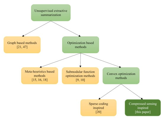
Figure 1.
A taxonomy of the unsupervised extractive summarization algorithms. We restrict to the most relevant methods.
Another way to approach this is to formulate the summarization as a submodular function maximization problem [9,10]. This approach proved to be quite useful from practical and theoretical standpoints. It is similar to ours, in the way that it tackles the summarization from an optimization perspective.
The paper [11] and some related contributions of the respective authors [12] share some ideas with our work. The common point is the use of convex optimization and the norm for text processing. Our goal is different both in purpose and method. In [11], the authors attempted to extract the relevant parts from a text corpus, where the relevance is concerning some keywords. To this end, they have defined the task as a feature selection problem and aimed to take advantage of the properties of the LASSO regression and -penalized logistic regression [13]. On the other hand, our work deals with the standard extractive summarization problem using an approach based on formulating more directly a convex program with constraints.
Another broad family of summarization techniques that uses optimization is the one based on meta-heuristics. For example, in [14], an algorithm based on differential evolution in proposed, while in [15], the authors apply fuzzy evolutionary optimization modeling. Another method from this category used with success for extractive summarization is the memetic algorithm [16]. A meta-heuristic method designed for speed is the micro-genetic algorithm [17]. The algorithm is faster than the standard genetic algorithm, mainly due to its smaller population size. It was employed for text summarization in [18]. While most of the algorithms from this category do not have formal convergence guarantees, simple stopping criteria, like the number of generations or objective function evaluations, work very well in practice [16,18,19]. These approaches often perform very well in terms of execution time and quality of the solution.
Probably the closest work to ours is [20]. This method is based on sparse coding. It uses a similar formalization with the one proposed in the current paper. The main difference lies in the structure of the objective function and the optimization algorithm (the core optimization algorithm used in [20] is the coordinate descent). We shall discuss it in some detail after the current method is presented (see Section 5).
A widespread and successful summarization algorithm is TextRank [21]. It is a graph based method, in fact a variation of the PageRank algorithm used in web search engines. Besides its excellent performance, it has the advantages of being computationally efficient [3], easy to apply, and scalable; thus it is a good baseline. We have implemented TextRank using the same technology as for our algorithm; therefore, we are able to make some meaningful comparisons regarding the execution time and scalability. For a description of the algorithm, see Appendix B.
We end this section by mentioning several deep learning summarization methods against which we compare our method. Inspired by the neural language models used for automatic translation, in [22], an attention based method has been developed. The system is abstractive and gives competitive results on several tasks. An important class of neural networks applied to summarization are those based on sequence-to-sequence architectures [23,24]. These architectures usually consist of one or more recurrent neural networks (e.g., LSTMs—long short-term memory) that map an input sequence to an output sequence (e.g., the text to the summary). Despite some inherent problems, like the tendency to repeat, they can provide good results. The work [25] is also based on recurrent neural networks (specifically LSTM) but takes a more modular approach: first, the most important sentences are extracted, then they are compressed by removing some of the words. The sequence pointer-generator network, described in [26], is a hybrid between a simple sequence-to-sequence network and a pointer network. Another architecture applied for summarization is the multi-layered attentional peephole convolutional LSTM, a modification of the standard LSTM [27]. The network used in [28] makes use of a complex language model (“transformer language model”). Despite using a powerful and resources intensive approach, the method is not particularly good. A somehow different approach is that based on reinforcement learning [29]. The main advantage of this solution is that it does not require large amounts of training data. The methods based on deep learning often provide very good results but are complex and require large amounts of computational resources and usually also training data.
The current paper develops the initial ideas introduced in [3] (see also [1]). The main new contributions are the theoretical analysis, the optimization algorithm, the experiments on Cornell Newsroom Summarization Dataset and DUC 2015 Dataset, and the computation time analysis.
3. Problem Formalization
In this section we provide a formal description of the extractive summarization problem.
The summarization process has usually three parts: preprocessing, processing, and postprocessing. They roughly correspond to generating a representation for the text, extracting the most relevant parts, and converting them to text, respectively. This work is focused on the processing part but, for completeness, we also present in this section the other two steps, although they are not essentially original.
The method is summarized in Table 1 and described in detail in the following subsections.

Table 1.
The proposed method description.
3.1. Preprocessing
As illustrated in [3], the first step for text summarization is to preprocess the text (Figure 2). This part has been limited to some basic operations:
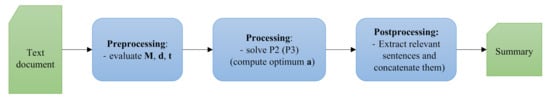
Figure 2.
Proposed method diagram. This paper concentrates on the processing step.
- Tokenization;
- Stop words removal;
- Conversion to lowercase;
- Stemming (with the Porter stemmer).
During the preprocessing phase we are interested in the numerical representation of the text and thus we will represent the text as a real matrix , where n is the number of sentences and m is the total number of distinct words, with each line associated with a sentence and each column representing a word, as in [3].
The specific computation procedure for the matrix entries may differ, but a usual method is Term Frequency—Inverse Document Frequency (TF-IDF) [30]. This is the method we have considered. Here, the raw meaning of an entry is that of the relevance of word j to sentence i. Similarly, the overall text can be represented by a vector with each element being the TF-IDF value for the word j.
The TF-IDF representation for each word is computed using the following formulas (the “corpus” is a set of documents; “doc” stands for a document from the corpus) [30]:
More concretely, the rows of are the (normalized) TF-IDF representations of the sentences, while is the (normalized) TF-IDF representation of the entire text (the document), multiplied by k, and is the (normalized) TF-IDF representation of the title (any deviation from this approach is explicitly mentioned in the text). In Appendix A, a concrete example is presented.
3.2. Processing
The idea of our method is to choose a maximum number of k sentences that best approximate the text when the above representation is used. In addition, it was noted that some additional properties of the sentences, as the length or the position in the text impact the decision to introduce them into the abstract [2,8]. This additional information is encoded into a vector , with positive real values.
In this context we can relatively simply formalize our approach (P1):
Here the sign stands for the matrix transposition operation and the other symbols are defined in the next paragraphs.
Each element of the vector indicates if the corresponding sentence (the i-th sentence) should be integrated in the summary () or not (). The parameter k is the maximum number of sentences we want in the summary. The pseudo-norm represents the number of non-zero elements of a vector (this is not a true norm since it does not satisfy the triangle inequality). The real value is non-negative. The parameter, together with vector , are user provided. They encode the influence of the “side information” we have, namely the a priori knowledge about the importance of different sentences.
As noted before, vector has positive values and their modulus shows the estimated importance of the corresponding sentences based on other criteria than the content of the sentences. Two widely used criteria are the sentence length and the position of the sentence in the document (see [8]). Since the effect of this side information depends on the dataset, we cannot give an explicit formula for the vector . It can be set by a trial and error method or using previous experience.
Let us observe that if ( is the orthogonal group) is an arbitrary orthogonal matrix, and we transform the representations of the text, and , using , the objective function is not affected: .
The program P1 has some resemblance with the ones found in the compressive sampling literature (the signal reconstruction phase) [4]. As in those cases, this optimization problem is NP-hard (see Section 6) and we shall speculate the properties of norm to find some approximation. To this end, we introduce the following convex relaxation (P2):
P2 is convex because the objective function and the feasibility set are convex (see Section 6 for details), thus P2 can be solved efficiently. Solving this convex program is the most critical part of the algorithm and represents the processing step.
3.3. Postprocessing
In the postprocessing step the summary is finally generated. The sentences associated with the greatest k non-zero elements in the vector are concatenate, in the original text order, as presented in [1]. If less than k values are greater than 0, we only use those.
Once generated, the summary can be further transformed to achieve a higher level of cohesion and compression using, for example, a sentence compression technique [31]. To avoid a loss of focus, we do not apply such transformations in this work.
3.4. Extending the Method
One important feature of this algorithm is that it is easy to be extended to use the problem structure or additional information. Indeed, if the title of the text is available, it can show us the relevant sentences. This can be integrated into the objective function by expressing the title as a regular sentence with a TF-IDF vector , and by reflecting its meaning in the selected sentences [3]. The method is formalized in the following program (P3):
where is another trade-off parameter, controlling the importance of the additional information (the other parameters are the same as in P2).
With the new program (P3) we can also perform query-based summarization (extract a summary which reflects a specified information or the answer to a question). In this case, the vector is computed, using the same procedure, from the text of the query.
We now turn our attention to the implementation of the processing step.
4. A Projected Gradient Descent Algorithm
The programs P2 and P3 can be solved using a general convex solver. However, our experiments revealed that they are too slow and affect the scalability of the system (see Section 7.1.2). To solve this issue we have applied the projected gradient descent framework to our problem. The main contributions of this section are the explicit formulas for the gradient and the projection operator. It turns out that in this case both of them can be computed very efficiently (see also Section 4.1).
Projected gradient descent is a class of first order optimization algorithms for constrained optimization problems. It borrows the essential properties of gradient descent. The most important property is the fact that under some conditions, it achieves the global optimum for convex problems and the convergence rate is the same with that of standard gradient descent. The main difficulty with this type of algorithm is that the projection can be very expensive. The good news is that in our case the projection can be done in time, following the approach proposed in [32]. The method consists in treating the projection as an optimization problem with a specific structure. The Lagrangian duality is used to reveal some properties of the solution which allow finding a solution in linear time.
However, this projection method is quite complex and better suited for the case when a high quality solution is required and computing speed is not a very stringent requirement. Note that the method is also the subject of a patent [33].
We make the remark that in our case the constraint is not very restrictive. In fact, a violation of no more than one does not affect the results. In addition, it was observed that a high tolerance is not problematic (see Section 7). With this observation in mind, we make one more change to the program P2 and replace the constraint with an additional term in the objective that will (approximately) enforce the constraint:
The parameter C can be chosen freely, and if it will be set to a large enough value, the solution of the new program P will be close to that of P2. The above program was introduced with the aim of making the projection step much easier: we now need to project the partial solution in the set defined by the box constraints, which is much easier than projecting in the feasible set of P2. With this modification, the objective function of P is still convex, since the last term is the multiplication of a positive scalar with a convex function. Projecting to the feasible set can be done in linear time. Now, we can proceed to derive an algorithm for this program.
Projected gradient descent is an iterative algorithm and each iteration consists in two main steps: the solution update in the opposite gradient direction and the feasible region projection. The first goal is to compute the gradient of the objective function of P:
where
Here we denote by f the objective function of program P.
The optimal step size (the value of the step that gives the greatest decrease of the objective function in the current iteration, ignoring the constraints) for our quadratic objective is given by:
Since can be singular, the step is not well-defined. To avoid this problem we observe that the constraints will force the solution to remain in the interior of the n-dimensional hypercube, which has the diagonal length . Therefore, we can naturally impose an upper bound on the step-size:
If or the limit is exceeded, the step-size is set to the maximum value. Since the step we take is never bigger than the best one, the objective function of P will always decrease; we cannot “overshoot”. The step is also large enough to get progress.
As expected, the solution is updated in the opposite direction of the gradient and the change is provided by the following relation:
After “the gradient update”, the new vector may be outside of the feasible region. The projection step will ensure that we find a feasible point that is as close as possible to our current candidate solution (with respect to the Euclidean distance).
Projecting in the box constraints works like this: for every ,
Here, the key observation is that each constraint depends on a different variable.
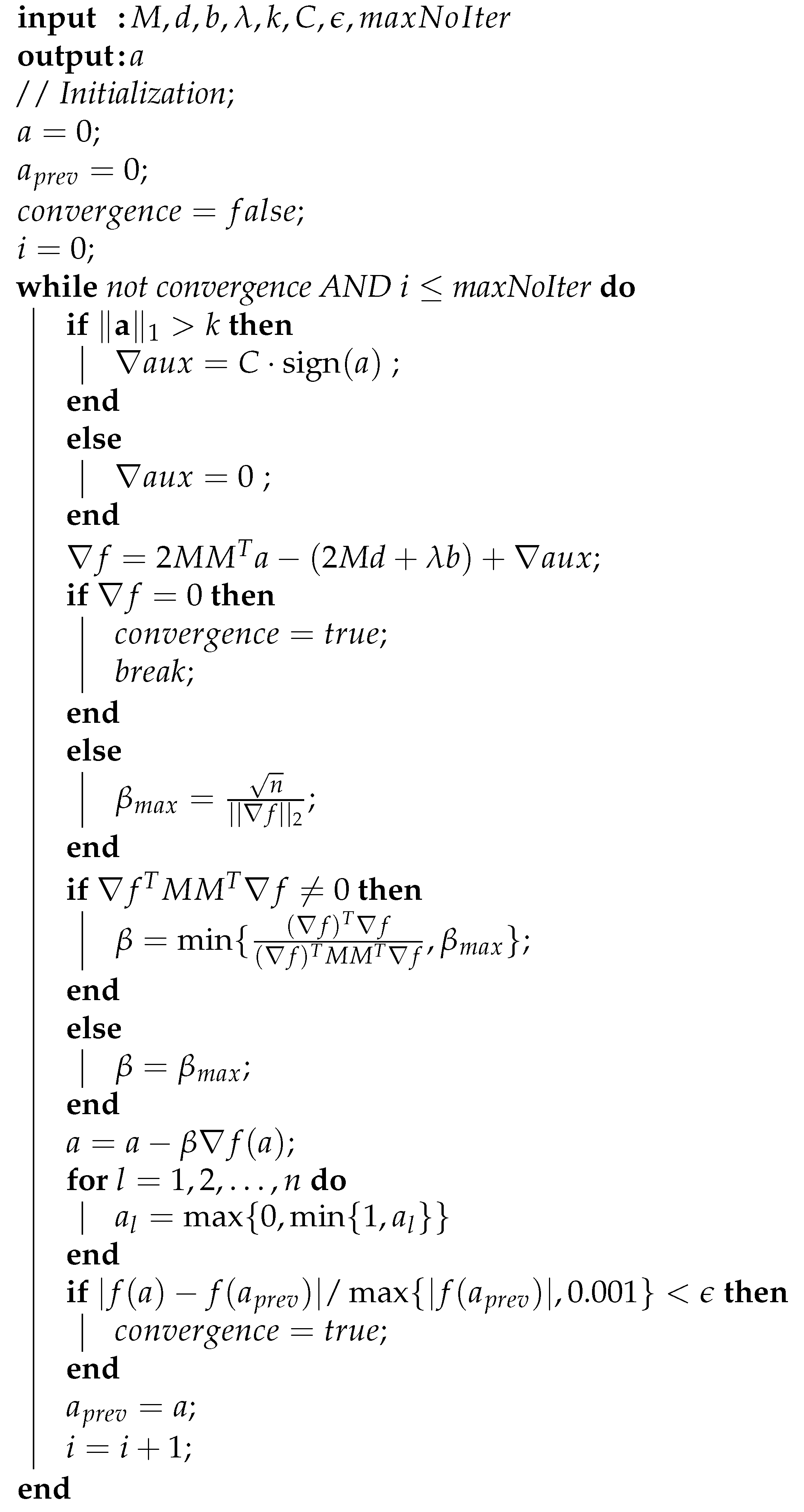
We synthesize this section in Algorithm 1. In addition to the model specific parameters already discussed, three new ones need to be provided:
- 1.
- the convergence tolerance ;
- 2.
- the maximum number of iterations ;
- 3
- the enforcement parameter C.
Their meaning is self-evident and in Section 7 we will discuss how can they be chosen.
In Algorithm 1 we focused on clarity rather than efficiency. On the other hand, in our implementation we tried to do the computations in the most efficient possible way. As an example, for the gradient update Formula (8), the matrix product () and the matrix vector product () can be computed before the “while” loop.
Note also that the approach can be easily adapted for program P3 and other similar optimization problems. We also employ in our experiments a version of the algorithm with fixed step. The new algorithm is identical with Algorithm 1, except that is a user-supplied (provided) parameter.
Algorithm 1 differs from the projected gradient descent applied to P2 in two respects: the projection is to a set defined only by the box constraints, and the gradient has the additional component . We measured the time needed for box constraints projection and the computation of and the time needed for a projection in the ball. For a vector with 1,000,000 entries, the average time needed for box constraints projection and , is 0.024 s. For the same vector, a projection step in the ball takes 0.096 s (The experiments were performed on a machine with Intel(R) Core(TM) i7-9850H CPU @ 2.60 GHz and 2.59 GHz RAM. The values are averages over 100 executions). If the projection is being performed in the intersection of ball and the set defined by the box constraints, the time will be even longer (for vectors of length 1,000,000, in [32], Section 5 Experiments, a value of 0.22 s was indicated).
4.1. Considerations about the Running Time
Here we will discuss the computational complexity of the summarization method (with all its components, not just the optimization part).
All the algorithms used for preprocessing are linear in the size of the input. The most demanding step from a computation point of view is to solve the convex optimization problem, but this still can be achieved in polynomial time. When this is done with an off-the-shelf solver, the general analysis of the specific algorithm and its implementation apply also in our case (see Section 7, references [34,35]). However, for most practical situations, this type of solver is too slow.
The projected gradient decent has the same convergence speed as simple gradient descent and is therefore linear (in the sense that the distance to the optimum shrinks as ). When computing the gradient, the most expensive operation is the evaluation of , which has a time complexity of or a little better with faster algorithms. Note that this operation should be done only once. During the iteration, only simpler computations are required. The dominating operation is the matrix vector multiplication, which requires time. For the numerical operations we use the built-in routines from NumPy which are known to be highly optimized. Finally, as we already observed, the projection to the feasible set only requires operations.
To find the largest entries in the solution, we sort the vector, and this takes time.
In order to have a better image of the computational effort required by our method, let us look also at TextRank complexity. This algorithm requires the construction of a similarity graph. This can be achieved in quadratic time. In the case of TextRank, the main computational task is the repeated matrix multiplication, which is performed until convergence is reached (usually in fewer than 200 steps). The size of the matrix is , thus an iteration step is in (cubic in the case of the naïve approach).
| Algorithm 1 Projected gradient descent (PGD) algorithm for P2 |
 |
5. The Relation with Sparse Coding
In [20] a technique based on sparse coding was introduced for a problem similar to the one discussed in this paper. In the following paragraphs we shall discuss the relation between that technique and our work.
The main purpose of [20] was to develop a method that uses the comments in the summarization process. To this end, the authors use the standard sparse coding method, which is related to the idea of compressive sensing.
However, their approach differs from ours in its goal (reader-aware vs. common/query-based text summarization), its starting point (we try to directly select the best sentences for the summary, while they use the sparse coding to compute one salience indicator for each sentence), and the final optimization problem. Besides this, we focus on the information retrieval part and try to decouple the linguistic processing from the information extraction.
There are also a few smaller differences. They use term-frequency representations; therefore, the relevance of the terms is not taken into account. In addition, the additional information is used by multiplying (with a constant) the term in the objective function, corresponding to the sentence.
The sparse coding is used to extract an expressiveness score which is then combined with the “concept score” that reflects the importance of a term to the topic. In contrast, we try to extract the sentences directly and the solution of the optimization program is interpreted as an indicator vector. Next, we will briefly show by using a toy model that starting from this point of view, the sparse coding idea is not appropriate—it leads to bad coverage and diversity.
Let us assume that we have in our corpus n sentences and two topics, the first topic having m sentences. Usually, the representations of the sentences that are part of the same topic are similar and very different from those belonging to the other topic. To better illustrate our point, we will assume that all vectors representing a topic are identical, of unit length and orthogonal to the ones from the second topic. Let be the vectors for the first topic and the vectors for the second topic. Using the observation that they are all identical for each topic, we denote by the vector for the first topic and by the vector for the second one ( and ).
Now, considering that the summary should have at most two sentences and following our idea of using as an indicator vector (the entries are 0 or 1), we will try to establish what sentences will be extracted using the two approaches.
The objective function for sparse coding looks as follows [20]:
It is easy to see that by taking only one sentence from the first topic, the objective function will have the value . If we take only one sentence from the second topic, the objective becomes . Taking two sentences from the same topic is worse. By picking one sentence from each topic the objective will be n. Therefore, if m is slightly smaller or slightly greater than , the algorithm only extracts one sentence. This is not so good, because both topics are almost equally well represented.
We now turn our attention to the objective function introduced here with this:
It is obvious that with this objective function, the algorithm will prefer to select one sentence from each topic as long as each topic has at least one quarter of the sentences. If a topic is below this threshold, and thus quite insignificant, the algorithm will select two sentences from the dominating topic. This shows why we prefer this approach rather than the sparse coding one.
6. Properties of the Optimization Problems
Through this section we will present and justify more formally some ideas that we have already mentioned, namely that solving P1 is difficult, solving P2 (or P3) on the other hand is feasible, and that between a solution of P1 and a solution of P2 there are some interesting connections.
6.1. Solving P1 Is NP-Hard
This can be easily shown by reducing from the known NP-complete problem “subset-sum” [36]. The most useful variant of the problem is this:
Problem 1.
Given some set S of positive integers and an additional positive integer s, decide if there is a subset of S that sum to s.
Starting from an instance of “subset-sum” we can construct a particular form of P1 with , , , (in this work stands for the cardinality of the set S). The matrix (now with only one column) has as elements the values in S and (d is now just a scalar).
We assume that there is an efficient algorithm for P1. If the optimum is equal to zero, then in S exists a subset that sums to s. If the optimum is larger than 0, then no such subset exists. Note that the optimum cannot be less than 0. Therefore, we can efficiently decide the problem “subset-sum”. Hence we established the NP-hardness of P1.
6.2. The Program P2 Is Convex
Convexity of the objective function of P2 results as a sum of a squared norm of a linear vector function and a linear scalar function. The box constraints are also convex, and so is the norm [3]. A direct consequence of convexity is the polynomial time solvability [37].
It is not difficult to show that the program is also quadratic. The following equalities provide an alternative way to write the objective function that will make obvious this property:
The quantity does not depend on vector , thus we can write the program P2 as a quadratic program in the canonical form:
Since is symmetric and positive semidefinite, this reformulation gives another proof of convexity of the program P2.
The quadratic nature of the program is important since solving a convex quadratic program is easier than solving a general convex program. This fact gives an additional motivation for using the norm.
6.3. The Optimal Value of P2 Is a Lower Bound for the Optimal Value of P1
Let us observe that the objective function is the same, and the feasible set of P1 is included in that of P2: if and , then .
This is a useful fact since it gives us an upper bound on the approximation error.
6.4. Under Some Conditions the Solution of P2 Is Close to a k-Sparse Vector
As noted before, our convex program is similar to some formulations of the reconstruction phase of a compressed sensing system. In the compressive sampling literature, the formal statements on the performance of the reconstruction algorithms are based on some specific assumptions regarding the matrix , like restricted isometry property [38]. In our case such assumptions do not hold, not even as a rough approximation, because we have a lot of correlations between words and between sentences. Instead we can use other properties which are natural in this setting.
In this subsection we will consider to be 0. Moving to the general case requires only some technical modifications and from our point of view does not bring any substantial contribution to the problem understanding.
This part should be regarded as a step towards giving an explicit and meaningful bound on the approximation error of the convex relaxation procedure. In this work we limit to this first step and to this end we introduce the following program (P4):
It differs from (P1), when , in only one respect: the variables are not binary but rather real values from the interval . The solution of P1 will be approximated by rounding to 1 the non-zero elements in the solution of P4 (see also Figure 3).
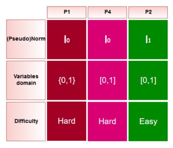
Figure 3.
Schematic view of the discussed programs.
One should notice that any feasible solution of P4 is k-sparse (it has at most k non-zero entries). Therefore, it is enough, for our current goal, to bound the distance between the solutions of P2 and P4.
Let be a solution of P2, a solution of P4, the error vector, and . If the matrix is not the zero matrix, is its largest singular value, and is its smallest non-zero singular value, the following inequality is true:
Proof.
We will bound the norm of the error vector by decomposing the vector along the row space of () and its orthogonal complement—the null space ().
If is the component in the null space, and is the component in orthogonal complement, by Pythagorean theorem we have:
We now proceed to bound each term.
- 1.
- Bounding .
We will make use of Lemma 10.6.5 from [7].
Claim 1. Lemma 10.6.5 in [7] .
For completeness, we reprove the result here using our notation. It follows from the definition of , that P2 and P4 have the same objective function and the feasible set of P4 is included in the feasible set of P2.
By definition, . Therefore, we have
If we take into account that , we have
and by taking the square,
The left-hand side of (23) can be rewritten as
Using the definition of and the Claim 1 we have:
Further, by Cauchy–Schwarz inequality and the definition of we can write
The quantity can also be lower bounded:
Therefore, we have
- 2.
- Bounding .
For this term we will look at the length of the vectors. The main idea can be stated as follows: since the norm of the solution is bounded, if the optimal value of the objective function is small, and the multiplication by matrix does not increase the norm too much, the orthogonal component cannot be large.
If does not have a null space, we have . We will now focus on the more interesting case that occurs when the null space has a dimension .
Let be an orthonormal base for . Then, the components of and belonging to this subspace can be written as:
and
for some coefficients and .
Since , we have
It follows that
(in (33), second row, the Cauchy–Schwarz inequality was used).
By triangle inequality and the definition of , we have:
Combining the above inequality with the fact that we get:
Using again the Pythagorean theorem, the inequality between the and norms, and the constraint , it follows that
Because , we can repeat the above steps, starting with (34), to also bound in the same way. Therefore, we have
which together with , will imply
Let us observe that from the definition of , we know that the value is greater or equal to 0.
- 3.
- Bounding .
In general the inequality can be loose. However, in our case, if we choose some representations such that , and a good summary exists (), the error will be small.
At this point we make a few observations. Usually the measurement matrix used for compressive sensing is generated randomly. On the contrary, in our case the matrix is computed based on the available data and cannot be modeled well by a random matrix with entries having strong independence properties. This is the reason why our results differ from those in two respects:
- 1.
- The bound is deterministic, not “with high probability”;
- 2.
- The bound is in a sense weaker, because we do not guarantee perfect reconstruction in the noise free case (). The bound can be in general quite loose, but if our assumptions and intuitions are true, this is not the case.
Another important observation is that from this proof results that a bound on the norm of vector can be just as good. However, the norm has other benefits, like its intuitive appeal and simplicity of the resulting optimization problem.
It remains to show also that the k-sparse vector generated from the solution of P2 can be easily found and it is a good approximation for the solution of P1. For now, the main conclusion of this section is that the vector we obtain by solving P2 has some properties that indicate it can be a decent solution for the original problem.
7. Implementation and Results
The Python programming language was used to implement the proposed solution. The main reason is given by its good features for both linguistic and numerical computation. To perform the preprocessing the popular natural language processing library NLTK (Natural Language Toolkit) [39] was used. We have considered the NumPy [40] and SciPy libraries [34] for the numerical computation part and Matplotlib [41] for generating figures.
All experiments were performed on a computer with an Intel(R) Core(TM) i7-3632QM CPU (2.2 GHz) and 8 GB of RAM.
In order to test our method we employed a series of experiments on artificial and real data. We start by evaluating the quality of the approximation and the execution time for the proposed relaxation method (in particular Algorithm 1). We then proceed to evaluate the method on two different tasks: single document summarization and query-based multi-document summarization.
The evaluation was based on the ROUGE (Recall-Oriented Understudy for Gisting Evaluation) tool which became the de facto standard in this field [42]. If not otherwise mentioned, we used the default settings, but we granted stemming and stop words removal. In all experiments the metrics for the entire dataset are computed as arithmetic means of the metrics for individual summaries generated by ROUGE.
7.1. Quality of the Approximation and Execution Time
In this section we try to answer empirically two questions:
- 1.
- What is the execution time of our method for different problem sizes?
- 2.
- How good is the approximate solution provided by Algorithm 1?
In order to evaluate our method we have implemented a brute force solver for P1. The program is solved exactly by searching through all possible solutions (e.g., if and , all binary vectors of length 4 with 2 entries set to 1). The algorithm has an exponential time complexity; therefore, it can only be run on some small problems. Since it has been shown in Section 6 that P1 is NP-hard, it is unlikely that an efficient solver exists.
To show the advantages of using the Algorithm 1, we have run some experiments with an “off-the-shelf” solver from computing library SciPy [34]. The solver is based on the “constrained optimization by linear approximation (COBYLA)” method [35], an approach that supports inequalities constraints.
The experiments are carried on both synthetic and real data. For the synthetic data, unless stated otherwise, the data matrix and the vector were generated randomly by sampling independently each entry from the uniform distribution over the interval . The values are computed by repeating 20 times the execution for each problem size and method and then taking the average.
7.1.1. Quality of the Approximation
Now we turn to the question of the quality of the approximation produced by our relaxation method. In order to shed some light on this problem, we solve exactly the program P1 using the brute-force algorithm, as it was noted earlier. This is possible only for small problem sizes, having a small number of sentences.
The approximate solution is obtained by solving the program P2 using the Algorithm 1 or the COBYLA based solver and by setting to 1 the k greatest entries in the solution and to 0 the rest of them. We then evaluate the objective function of P1 for the approximate and the exact solutions and compute the relative error (If is the objective function of P1, the exact solution, the approximated solution, then the relative error is ). The data is generated randomly, as it is described at the beginning of Section 7.1.2.
Quality of the Approximation as a Function of the Number of Sentences
Figure 4 and Figure 5 and Table 2 illustrate an interesting dependency of the error on the number of sentences for random data. Up to about 15 sentences, the error increases. After this threshold the error stabilizes at a reasonable value: 0.25–0.3 for 50 words and 0.05–0.06 for 1000 words. Note that both PGD (Algorithm 1) and COBYLA behave in about the same manner.
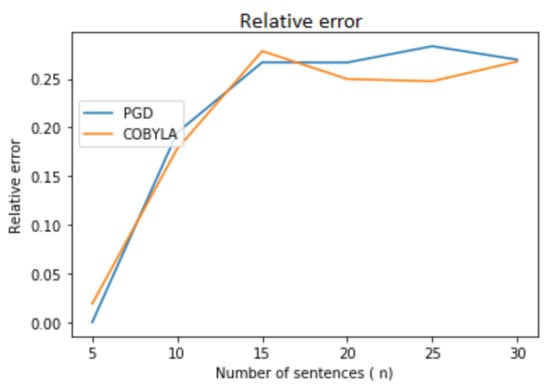
Figure 4.
Quality of the approximation as the number of sentences increases (number of words is 50). Comparison between our method (PGD) and an “off-the-shelf” method (COBYLA).
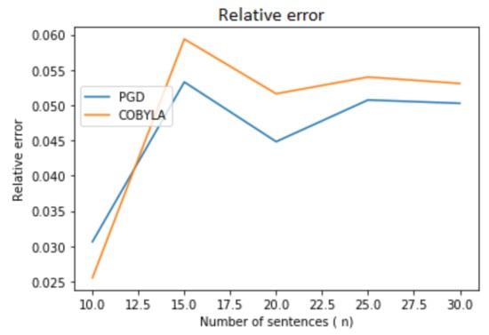
Figure 5.
Quality of the approximation as the number of sentences increases (number of words is 1000). Comparison between our method (PGD) and an “off-the-shelf” method (COBYLA).
Table 2.
Quality of the approximation as the number of sentences increases (number of words is 1000). Averages over 20 executions. Comparison between our method (PGD) and an “off-the-shelf” method (COBYLA).
Quality of the Approximation as a Function of the Number of Words
For both our algorithm and the off-the-shelf solver, the quality tends to increase fast when the size of the vocabulary grows (see Figure 6 and Table 3). It is worth noting and may be due to the random nature of the data in these experiments. One important point, however, is that the two algorithms have about the same outcome.
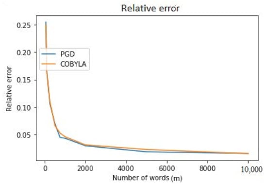
Figure 6.
Quality of the approximation as the number of words increases (number of sentences is 20). Comparison between our method (PGD) and an “off-the-shelf” method (COBYLA).
Table 3.
Quality of the approximation as the number of words increases (number of sentences is 20). Average over 20 executions. Comparison between our method (PGD) and an “off-the-shelf” method (COBYLA).
Quality of the Approximation for Real Data
In Figure 7 we illustrate the behavior of the relaxation procedure for some real texts (the first 100 documents from [43]). In order to compute the error, we need to know an optimal solution. Therefore, we have truncated the texts to the first 20 sentences (the summary has 5 sentences), so we can use the brute-force method. What we have observed is that the error is in general relatively small, less than 1, both for PGD and COBYLA. COBYLA has an advantage though, the average error being around 0.3, while for PGD it is about 0.6; this is due to a few examples in which the algorithm fails to find a good value.
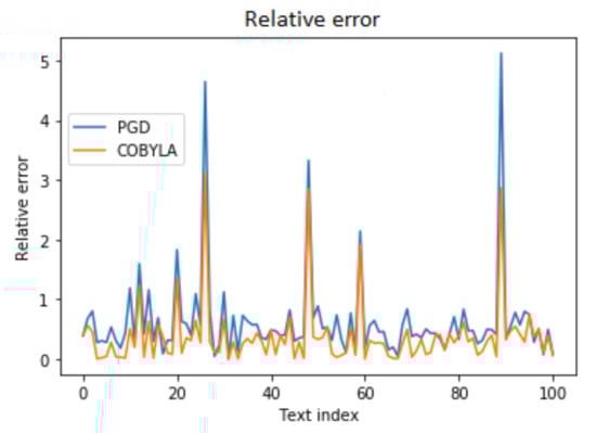
Figure 7.
Quality of the approximation for real data.
7.1.2. Execution Time
This section is dedicated to the investigation of the speed of the method.
Execution Time as a Function of the Number of Sentences
The first experiment addresses the problem of execution time of Algorithm 1. The data is generated randomly (using the same method as above), the number of words is kept fixed at , and the summary length is a quarter of the number of sentences.
The results are summarized in Table 4. The brute-force method only works for a relatively small number of sentences; beyond , it becomes impractical. In Figure 8 we can see the exponential growth of the execution time for the brute force method (the plot is on the double logarithmic scale). On the other hand, the behavior of the baseline method and our algorithm is much better: for 1000 sentences, the execution took only 2.256 s and respectively 0.016 s.
Table 4.
Execution time (in seconds) as a function of the number of sentences for the brute-force, an “off the shelf” convex solver (COBYLA), and the algorithm presented in this paper (PGD—Algorithm 1). The results are for a vocabulary of words and long summaries. The numbers are averages over 20 executions.
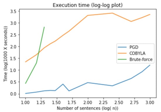
Figure 8.
Variation of the execution time when the number of sentences increases (for both axes a logarithmic scale is used). Comparison between our method (PGD), an “off-the-shelf” method (COBYLA), and the “brute-force” approach (which could be run only for small instances).
Execution Time as a Function of the Number of Words
The size of the vocabulary is much less important for the execution time. Figure 9 and Table 5 show that all methods scale to very high dimensional tasks. The data was generated as in the previous experiment.
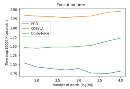
Figure 9.
Variation of the execution time when the number of words increases. Comparison between our method (PGD), an “off-the-shelf” method (COBYLA), and the “brute-force” approach.
Table 5.
Execution time (in seconds) as a function of the number of words for the brute-force, an “off the shelf” convex solver (COBYLA), and the algorithm presented in this paper (PGD—Algorithm 1). The results are for sentences and long summaries. The outcomes are averages over 20 executions.
Execution Time for Different Document Lengths—Experiments with Real Data
We investigated the execution time of the entire summarization program on a real text: the novel War and Peace by Lev Tolstoy [44]. During the experiment, the text is truncated at different numbers of words.
A number of observations can be made. As the length increases, both the vocabulary and the number of sentences increase, at least in principle. However, after a threshold almost all words are in the vocabulary; therefore, it grows very slowly. On the other hand, the number of sentences continues to grow at about the same rate.
Now let us recall from Section 4.1 that the computation is dominated by the iterative component and a step in the loop of Algorithm 1 requires operations. If we assume that the size of the vocabulary is essentially constant, we end up with a linear behavior. This is exactly what we see in Figure 10. On the other hand, for the baseline (TextRank) we have a quasi-quadratic complexity in the number of sentences (we refer again to Section 4.1). This conclusion is thus well verified empirically (see Figure 10 and Table 6).
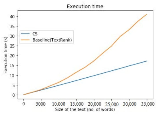
Figure 10.
Execution time of the summarization program for real data. The texts are generated by truncating the novel War and Peace at different numbers of words. Note that the number of sentences also increases.
Table 6.
Execution time (in seconds) of the proposed method in comparison with TextRank (the baseline), when the size of the document (number of words) increases ( no_words).
7.2. Single Document Summarization
In what follows we present a number of experiments on two datasets. The results are compared with those reported in the literature.
7.2.1. Experiments with a Medium Size Dataset
In our first experiment we used as data a collection of 4515 news articles (with the associated human produced summaries) publicly available [43]. The dataset (which, for convenience, we will call NEWS DATASET) has some useful properties: the title is available for each article and in addition the abstracts have approximately the same number of sentences.
We can place the difficulty of the task between summarizing a scientific article, which has a lot of structures and keywords, and that of summarizing a literary text with free and unexpected structure and commonly having lots of common words with context specific meaning.
Before proceeding to the formal evaluation, let us look at a few examples of summaries. The first three are for an article with the headline “Congress opens ’State Bank of Tomato’ in Lucknow”. The article was published in the online edition of the newspaper India Today and is the tenth text in the NEWS DATASET [43].
Example 1. 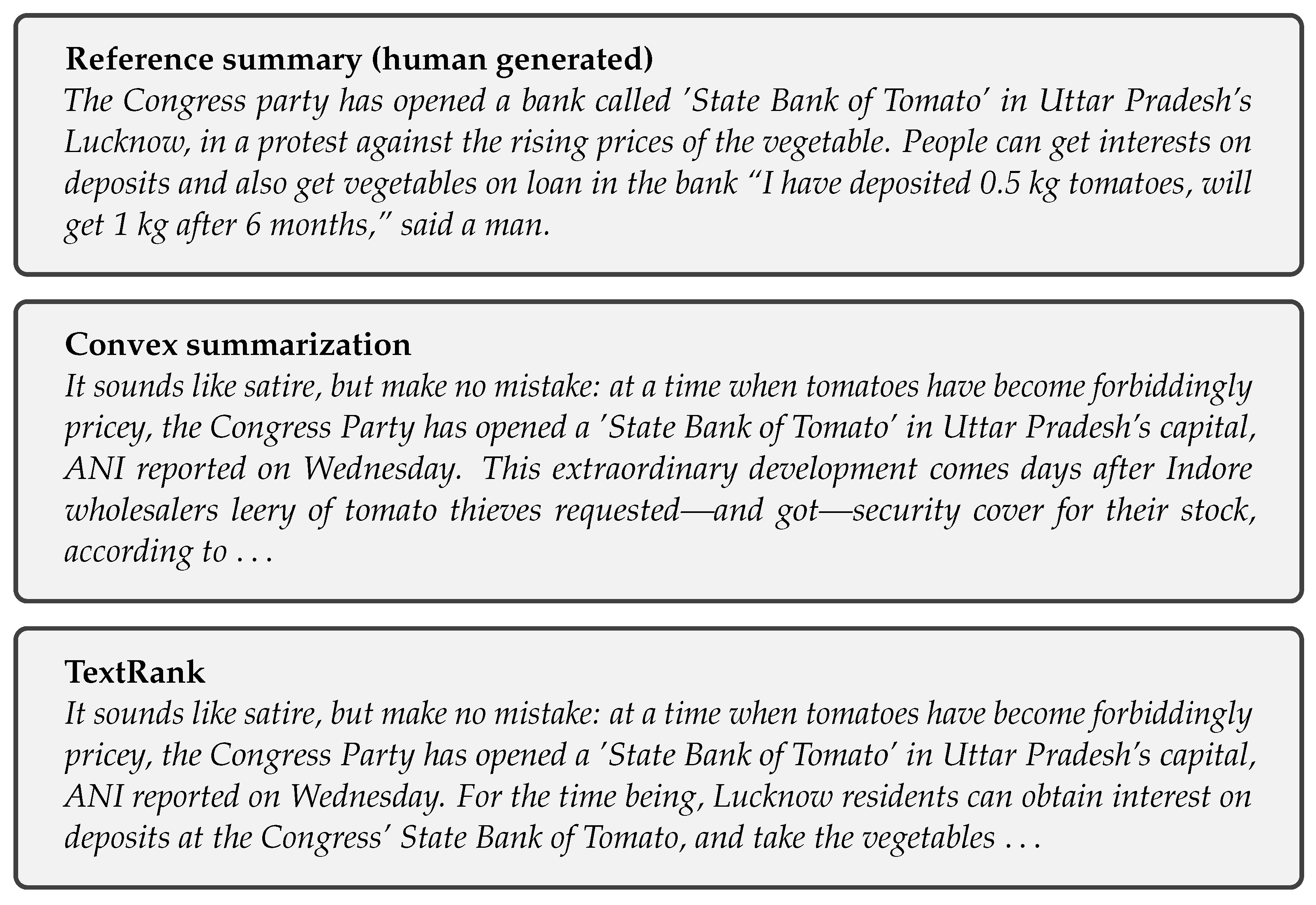
The next three are for an article called “World Bank downgrades India’s growth forecast after demonetisation” and were published by The Guardian in 2017. In the NEWS DATASET [43], it can be found as the text with number 1625.
In both examples, the generated summaries are constrained to have a number of words equal to that of the human generated summary.
Example 2. 
Regarding the length of the summaries, we talked about the number of sentences. From the readability point of view, this makes perfect sense since incomplete sentences may not be syntactically correct or may very well be meaningless. However, in the automatic evaluation procedure this approach can cause bias, because the evaluation is done at word level. Therefore, in order to have more meaningful results we now impose a bound on the maximum number of words (100 in all experiments from this section). Note that if the summaries are long enough, the distinction between the two approaches vanishes.
As we stated previously, we perform a direct comparison with TextRank. In our experiments TextRank performance is consistent with that reported in [21]. The ROUGE-1 F-score obtained by the authors on DUC-2002 dataset [45], for sentences extraction (100 words), without stop words and using stemming is 0.4229. In the same conditions and with respect to the same metric, on our dataset we get the slightly better value of 0.454.
In the first experiments, we have compared our algorithm CS (Convex Summarization) in its basic form with TextRank. Because TextRank cannot directly take advantage of the side information, we will also ignore it by setting . In this case, the algorithm performs slightly worse than TextRank (see Table 7, Table 8 and Table 9).
Table 7.
Results for different algorithms/parameters for ROUGE-1.
Table 8.
Results for different algorithms/parameters for ROUGE-2.
Table 9.
Results for different algorithms/parameters for ROUGE-L.
The next step is to study the impact of using side information. is set to 0.5 and in vector b the first three values are set to 1 and the last one is set up to 0.5. This selection is based empirically on the fact that these parts of the text tend to be more important. With these modifications, a significant improvement is noticeable for all metrics, CS outperforming TextRank (e.g., the F-score increases by more than 0.01). Most likely this can be further improved, using more carefully chosen values for and b.
Finally, we do a simple test using program P3, setting and as in the previous case and . We noticed that this change has a positive impact on the results (e.g., the F-score is with 0.03 greater than that for the basic version) without a significant increase in the computation time.
Table 7, Table 8 and Table 9 summarize the results: precision, recall, and F-measure are presented for all algorithms. The highest values obtained are italicized, to easy identify the winner algorithm. As it can be noticed, the winner is CS with P3, , and .
The computation time of the method on this dataset is about 11 min, nearly half of that of the current implementation of TextRank (which is about 20 min). Most of the time is spent on computing the IDF scores, thus for further reducing this value a modification of that part is needed.
Although the comparison was done directly with only one algorithm, since we generated the metrics with a tool (ROUGE) used by almost all researchers, we can indirectly perform a row comparison with other algorithms reported in the literature.
In the next section we evaluate the algorithm on a widely used dataset, and this will enable us to compare the results with those reported for other methods.
7.2.2. Experiments with a Large Dataset (CORNELL NEWSROOM)
Cornell Newsroom is a large dataset for evaluating summarization systems [46]. The key feature of the dataset is its size: it contains 1.3 million articles and abstracts written in the editorial offices of 38 major publications by authors and editors. The summaries are generated from (search and social) metadata between 1998 and 2017 and use both extraction and abstraction summarization strategies. In contrast with the experiments described above, in this set of experiments we focus on getting the best results rather than evaluating the effects of different parameters or data properties.
In order to compare our system with the others that have been tested on the dataset, we have run our algorithm on the “released test data”, consisting of about 100,000 text-summary pairs. The parameters were set as follows: , , , the first 3 values of the vector were set to 1 and the remaining values to 0, the step size was fixed to a maximum of and the maximum number of words was 30.
The evaluation methodology was the same used for the other algorithms tested on this dataset [46]. We have computed the F1-score (harmonic mean) of the ROUGE-1, ROUGE-2, and ROUGE-L metrics, without using stemming and without removing the stop words. Based on this, our system has average performance (see Table 10), but most systems are much more complex and require training [22,23,24,25,26,28,29].
Table 10.
Results for Cornell Newsrooms dataset. Three algorithm types are available: Unsupervised Extractive (UE), Supervised Mixed (SM), and Supervised Abstractive (SA) [46]. Note that the last two types require training.
Our system outperforms TextRank, on all metrics, by a distinct margin (R-1 = 0.3054, R-2 = 0.1868, R-L = 0.2234 vs. R-1 = 0.2445, R-2 = 0.1012, R-L = 0.2013). A surprising feature of the dataset is the very high score of a simple baseline method—Lede-3 Baseline. This could be a consequence of the fact that many abstracts were generated in an extractive manner. Because the same procedure is used by Lede-3 Baseline, this leads to very high scores of the method on this subset (R-1 = 0.53, R-2 = 0.49, R-L = 0.52—these are the values for extractive generated reference summaries, while in Table 10 the values are for the entire dataset). On the other hand, for the other summaries the values are smaller [46].
7.3. Query-Based Multi-Document Summarization
In this section we present some experiments on a more complex setting: multi-document query based summarization.
The dataset used is DUC 2005, one of the standard corpora in this research area [48]. This dataset contains 50 collections (“topics”) of news articles of 25–50 related documents each. For every document set a short (1–3 sentences) query (“narrative”) is supplied alongside other information (the headline of the article, for instance). Between four and nine reference summaries are supplied for every collection and the target summary size is 250 words.
For this task we use program P3, solved using a slightly modified version of Algorithm 1. The common data dependent quantities are computed as for single document summarization, with the difference that all texts from a collection are concatenated to form a single document. The vector is now used to provide the query information (we attempted to also use the headline, but it did not help). More precisely, is computed from the query text using the same preprocessing steps and the TF-IDF algorithm.
The parameters of the algorithm are: , , , , , (tolerance). As in the DUC2005 experiments, we limit the length of the summary to 250 words. The only two ad hoc modifications were to scale the document vector by a factor of 2 and to impose a limit on the step size of 0.001.
The evaluation is done also with the ROUGE tool. In Table 11 we compare the ROUGE-1 scores. We tried to reproduce the same setup used for the original DUC2005 evaluation (so without stemming and stop words removal). The DUC 2005 results are taken from [49] (see also the paper [48] for a description of the methods used).
Table 11.
ROUGE-1 scores on DUC 2005. For details about the methods see [48,49] and references therein.
In Table 12 we compare the ROUGE-2 scores. This time the evaluation is performed using stemming but without removing the stop words. The results are from [50]. In the same paper the scores for the ROUGE-SU4 metric are presented, and we summarize them in Table 13. These are calculated within the same conditions.
Table 12.
ROUGE-2 recall on DUC 2005. For details about the methods see [48,50] and references therein.
Table 13.
ROUGE-SU4 scores on DUC 2005. For details about the methods see [48,50] and references therein.
We make the remark that in our experiments, we use ROUGE 2.0 instead of the older ROUGE-1.5 employed for DUC2005 evaluations. The version considered in this paper does not perform bootstrapping/jackknifing, thus there might be some differences on the reported scores, if the version 1.5 is taken into account. However, this is unlikely to be significant.
Based on these outcomes, our method compares favorably with the methods developed for DUC2005 and with some newer algorithms, like the one introduced in [49]. Note that the top results are obtained with rather computationally intensive algorithms that rely on linguistic resources (like WordNet [51]). On the other hand, we do not focus on some properties of the summaries that were analyzed manually on the DUC 2005 conference, like coherence and readability.
The method turns out to be quite fast. Generating all the summaries takes about 6–7 min. As in the previous experiments, most of the time is spent on vocabulary and IDF scores production.
8. Conclusions
Through this work, we have proposed a new algorithm for extractive text summarization based on some simple and intuitive ideas, and we have tried to establish its properties and performance.
Among the advantages of the presented method, we can underline the extensibility and the possibility to use side information and additional constraints.
The method is fast enough to scale to large datasets and can be used in multiple contexts, ranging from a simple single document to multi-document query-based summarization. The scalability was achieved by designing a specific optimization algorithm for the problem at hand. Its accuracy is comparable with that of a standard off-the-shelf method, but it is up to 100 times faster for large documents (see Section 7.1).
The empirical analysis was performed with synthetic and real data. For standard summarization, on the Cornell Newsroom dataset, the method surpassed other general algorithms of similar complexity. For query-based summarization, our tests on the DUC2005 dataset revealed that the method is competitive, placing among the first four algorithms when the comparison was done using the results reported in the literature.
In this paper, we focused on the information extraction part of the summarization process. A possible extension will be to try to integrate linguistic processing to improve the quality of the summary. Another direction for the future could be the summary of other types of documents, especially those of the medical type [52].
Finally, we want to emphasize once again that ideas and methods from compressive sampling (in particular sparse signal reconstruction) and convex optimization can be very useful in text mining, information extraction, and natural language processing.
Author Contributions
Conceptualization, C.P. and C.R.; methodology, C.P., L.G. and C.R.; software, C.P.; validation, L.G. and C.R.; formal analysis, C.P. and C.R.; investigation, C.P.; resources, C.P., L.G. and C.R.; writing—original draft preparation, C.P., L.G., and C.R.; writing—review and editing, C.P., L.G. and C.R.; visualization, C.P., L.G.; supervision, C.P., L.G. and C.R.; project administration, C.P., L.G. and C.R. All authors have read and agreed to the published version of the manuscript.
Funding
This research received no external funding.
Institutional Review Board Statement
Not applicable.
Informed Consent Statement
Not applicable.
Data Availability Statement
Not applicable.
Acknowledgments
This work was supported by a grant of the Romanian Ministry of Research and Innovation, CCCDI—UEFISCDI, project number 52/2020, PN-III-P2-2.1-PTE-2019-0867, within PNCDI III.
Conflicts of Interest
The authors declare no conflict of interest.
Appendix A. An Example of Text Representations Computation
In this appendix, a toy example is used to illustrate how matrix and vector are computed.
Suppose that we want to summarize this text: “A short text. A sentence about summarization. Another sentence about summarization. A last one.”, with sentences, into a text with only sentences. In order to get the IDF components, we assume that an additional text is available: “Some text.”.
Applying the steps described in Section 3 we get the following representations. The vocabulary will be (the numbers indicate the positions in vector and the columns of associated to each word):
The matrix has the following structure:
while the vector is:
Appendix B. TextRank
Since TextRank algorithm is considered as the baseline, we will briefly describe it in this appendix, focusing on the variant that we have used in our experiments. In order to make a meaningful comparison, the TextRank algorithm was implemented using the same technology. In our TextRank implementation we tried to follow to the fullest possible extent the description found in [21]. For reader’s convenience we will briefly describe the key components of the algorithm.
TextRank is based on the idea of representing the text as a graph. The graph is constructed by assigning a vertex to each sentence and then including an edge between two vertexes if the associated sentences have words in common. We use an undirected graph, and each edge has a weight computed as in Equation (A3).
where and represent sentences (interpreted as sets of words) and represents words.
The algorithm works by iteratively adjusting the relevance of the sentences and, after the convergence is reached, it extracts the most relevant ones. At each step, the relevance of each vertex of the graph () is adjusted based on the current relevances of its neighbours () and the weights of the graph ().
By and , we denote the set of vertices that point to vertex V and the set of vertices that vertex V points to, respectively (for undirected graphs they are the same).
Appendix C. Useful Convex Optimization and Signal Processing Notions
Convex optimization studies the problem of minimizing convex functions over convex sets [37]. It is important mainly because convex optimization problems can be solved efficiently.
In general, a convex program has the following form:
where are arbitrary natural numbers, is the optimization variable, f and are convex, and are affine. The set of points for which all constraints are satisfied is called the feasible set.
One of the simplest algorithms for optimizing an unconstrained convex objective is gradient descent. The algorithm consists of iterating the following update rule: , where is the gradient of the function, and , “the step” of the algorithm, is a positive value. If some constraints are present, the algorithm can be modified to take them into account. One way to do that is to project the new value in the feasible set, after each iteration. Here “projecting” means to replace by the closest point in the feasible set. The new algorithm is named projected gradient descent.
Convex relaxation is the technique of replacing a hard optimization problem by a convex program such that the solution of the new program gives information (e.g., a lower bound) about the solution of the original program. In this paper we focus on the specific case in which a discrete feasibility set is replaced by a convex set that contains it.
For an arbitrary vector , the norm is defined as , while the pseudo-norm is the number of non-zero entries in the vector x.
Compressed sensing is a signal processing technique for efficiently acquiring (in a compressed form) and reconstructing a sparse signal [4,7]. The acquisition phase consists of an incomplete set of measurements, while the reconstruction phase is based on solving a convex program. Usually, the objective function contains the norm of the signal. A large number of experimental and theoretical investigations [4,7,38] have shown that this norm promotes sparsity, improving the change of, or in some cases guaranteeing, the perfect reconstruction of the signal.
Appendix D. Different Approaches to Text Summarization
Currently, there are two main types of text summarization, extractive and abstractive [2,8]. They can be also combined in different ways, resulting in mixed summarization methods. One way to generate a mixed summary is to first perform extractive summarization, then simplify and rewrite the sentences (e.g., using ideas from [31]). This method can be used to enhance the algorithm presented in this paper.
The summarization methods can be also classified based on the required dataset. If a training dataset composed of text-summary pairs is required, we call it a supervised method. Otherwise, they are called unsupervised methods. In many cases the supervised methods are superior in terms of accuracy, but they require a training phase.
We sketch a comparison of the different methods in Table A1.
Table A1.
Summarization methods (UE-unsupervised extractive; SE-supervised extractive; UA-unsupervised abstractive; SA-supervised abstractive; UM-unsupervised mixed; SM-supervised mixed).
Table A1.
Summarization methods (UE-unsupervised extractive; SE-supervised extractive; UA-unsupervised abstractive; SA-supervised abstractive; UM-unsupervised mixed; SM-supervised mixed).
| Method | Training | Grammatical | New Words | Compression | Scalability | Complexity |
|---|---|---|---|---|---|---|
| UE | No | Usually | No | Medium–Low | Medium–High | Low–Medium |
| SE | Yes | Usually | No | Medium–Low | Medium–High | Medium |
| UA | No | Sometimes | Yes | Medium–High | Low–Medium | Medium |
| SA | Yes | Sometimes | Yes | Medium–High | Low–Medium | Medium–High |
| UM | No | Often | Yes | Medium | Medium | Medium–High |
| SM | Yes | Often | Yes | Medium | Medium | High |
References
- Popescu, M.C.; Grama, L.; Rusu, C. On the use of positive definite symmetric kernels for summary extraction. In Proceedings of the 2020 13th International Conference on Communications (COMM), Bucharest, Romania, 18–20 June 2020; pp. 335–340. [Google Scholar] [CrossRef]
- Nenkova, A.; McKeown, K. Automatic Summarization. Found. Trends® Inf. Retr. 2011, 5, 103–233. [Google Scholar] [CrossRef] [Green Version]
- Popescu, C.; Grama, L.; Rusu, C. Automatic Text Summarization by Mean-absolute Constrained Convex Optimization. In Proceedings of the 41st International Conference on Telecommunications and Signal Processing, Athens, Greece, 4–6 July 2018; pp. 706–709. [Google Scholar] [CrossRef]
- Candes, E.J.; Wakin, M.B. An Introduction To Compressive Sampling. IEEE Signal Process. Mag. 2008, 25, 21–30. [Google Scholar] [CrossRef]
- Tibshirani, R. Regression Shrinkage and Selection via the Lasso. J. R. Stat. Soc. Ser. B 1996, 58, 267–288. [Google Scholar] [CrossRef]
- Uthus, D.C.; Aha, D.W. Multiparticipant chat analysis: A survey. Artif. Intell. 2013, 199–200, 106–121. [Google Scholar] [CrossRef]
- Vershynin, R. High-Dimensional Probability: An Introduction with Applications in Data Science; Cambridge University Press: Cambridge, UK, 2018. [Google Scholar]
- Allahyari, M.; Pouriyeh, S.A.; Assefi, M.; Safaei, S.; Trippe, E.D.; Gutierrez, J.B.; Kochut, K. Text Summarization Techniques: A Brief Survey. arXiv 2017, arXiv:abs/1707.02268. [Google Scholar] [CrossRef] [Green Version]
- Hui Lin, J.B.; Xie, S. Graph-based submodular selection for extractive summarization. In Proceedings of the 2009 IEEE Workshop on Automatic Speech Recognition & Understanding, Moreno, Italy, 13 November–17 December 2009; pp. 381–386. [Google Scholar] [CrossRef]
- Lin, H.; Bilmes, J. Multi-document Summarization via Budgeted Maximization of Submodular Functions. In Proceedings of the Human Language Technologies: The 2010 Annual Conference of the North American Chapter of the Association for Computational Linguistics—HLT’10, Los Angeles, CA, USA, 2–4 June 2010; Association for Computational Linguistics: Stroudsburg, PA, USA, 2010; pp. 912–920. [Google Scholar]
- Jia, J.; Miratrix, L.; Yu, B.; Gawalt, B.; Ghaoui, L.E.; Barnesmoore, L.; Clavier, S. Concise comparative summaries (CCS) of large text corpora with a human experiment. arXiv 2014, arXiv:1404.7362. [Google Scholar] [CrossRef] [Green Version]
- Miratrix, L.; Jia, J.; Gawalt, B.; Yu, B.; Ghaoui, L.E. What Is in the News on a Subject: Automatic and Sparse Summarization of Large Document Corpora; UC Berkeley: Berkeley, CA, USA, 2011; pp. 1–36. [Google Scholar]
- Hastie, T.; Tibshirani, R.; Friedman, J. The Elements of Statistical Learning—Data Mining, Inference, and Prediction, 2nd ed.; Springer: New York, NY, USA, 2011. [Google Scholar]
- Aliguliyev, R.M. A new sentence similarity measure and sentence based extractive technique for auto-matic text summarization. Expert Syst. Appl. 2009, 36, 7764–7772. [Google Scholar] [CrossRef]
- Song, W.; Cheon Choi, L.; Cheol Park, S.; Feng Ding, X. Fuzzy Evolutionary Optimization Modeling and Its Applications to Unsupervised Categorization and Extractive Summarization. Expert Syst. Appl. 2011, 38, 9112–9121. [Google Scholar] [CrossRef]
- Mendoza, M.; Bonilla, S.; Noguera, C.; Cobos, C.; León, E. Extractive Single-Document Summarization Based on Genetic Operators and Guided Local Search. Expert Syst. Appl. 2014, 41, 4158–4169. [Google Scholar] [CrossRef]
- Krishnakumar, K. Micro-Genetic Algorithms for Stationary and Non-Stationary Function Optimization. In Proceedings of the 1989 Symposium on Visual Communications Image Processing, and Intelligent Robotics Systems, Philadelphia, PA, USA, 1–3 November 1989. [Google Scholar]
- Debnath, D.; Das, R.; Pakray, P. Extractive Single Document Summarization Using an Archive-Based Micro Genetic-2. In Proceedings of the 2020 7th International Conference on Soft Computing Machine Intelligence (ISCMI), Stockholm, Sweden, 14–15 November 2020; pp. 244–248. [Google Scholar] [CrossRef]
- Saini, N.; Saha, S.; Chakraborty, D.; Bhattacharyya, P. Extractive single document summarization using binary differential evolution: Optimization of different sentence quality measures. PLoS ONE 2019, 14, e0223477. [Google Scholar] [CrossRef] [Green Version]
- Li, P.; Bing, L.; Lam, W.; Li, H.; Lia, Y. Reader-Aware Multi-Document Summarization via Sparse Coding. In Proceedings of the Twenty-Fourth International Joint Conference on Artificial Intelligence, Buenos Aires, Argentina, 25–31 July 2015; pp. 1270–1276. [Google Scholar]
- Mihalcea, R.; Tarau, P. TextRank: Bringing Order into Text. In Proceedings of the 2004 Conference on Empirical Methods in Natural Language Processing, Barcelona, Spain, 25–26 July 2004; pp. 404–411. [Google Scholar]
- Rush, A.M.; Chopra, S.; Weston, J. A Neural Attention Model for Abstractive Sentence Summarization. arXiv 2015, arXiv:1509.00685. [Google Scholar]
- Shi, T.; Keneshloo, Y.; Ramakrishnan, N.; Reddy, C.K. Neural Abstractive Text Summarization with Sequence-to-Sequence Models. arXiv 2018, arXiv:1812.02303. [Google Scholar]
- Shi, T.; Wang, P.; Reddy, C.K. LeafNATS: An Open-Source Toolkit and Live Demo System for Neural Abstractive Text Summarization. In Proceedings of the 2019 Conference of the North American Chapter of the Association for Computational Linguistics (Demonstrations), Minneapolis, MN, USA, 2–7 June 2019; pp. 66–71. [Google Scholar] [CrossRef]
- Mendes, A.; Narayan, S.; Miranda, S.; Marinho, Z.; Martins, A.F.T.; Cohen, S.B. Jointly Extracting and Compressing Documents with Summary State Representations. arXiv 2019, arXiv:1904.02020. [Google Scholar]
- See, A.; Liu, P.J.; Manning, C.D. Get To The Point: Summarization with Pointer-Generator Networks. In Proceedings of the 55th Annual Meeting of the Association for Computational Linguistics (Volume 1: Long Papers); Association for Computational Linguistics: Vancouver, BC, Canada, 2017; pp. 1073–1083. [Google Scholar] [CrossRef] [Green Version]
- Rahman, M.M.; Siddiqui, F.H. An Optimized Abstractive Text Summarization Model Using Peephole Convolutional LSTM. Symmetry 2019, 11, 1290. [Google Scholar] [CrossRef] [Green Version]
- Subramanian, S.; Li, R.; Pilault, J.; Pal, C. On Extractive and Abstractive Neural Document Summarization with Transformer Language Models. arXiv 2019, arXiv:1909.03186. [Google Scholar]
- Keneshloo, Y.; Ramakrishnan, N.; Reddy, C.K. Deep Transfer Reinforcement Learning for Text Summarization. arXiv 2018, arXiv:1810.06667. [Google Scholar]
- Salton, G.; McGill, M.J. Introduction to Modern Information Retrieval; McGraw-Hill, Inc.: New York, NY, USA, 1986. [Google Scholar]
- Knight, K.; Marcu, D. Summarization beyond sentence extraction: A probabilistic approach to sentence compression. Artif. Intell. 2002, 139, 91–107. [Google Scholar] [CrossRef] [Green Version]
- Gupta, M.D.; Kumar, S.; Xiao, J. L1 Projections with Box Constraints. arXiv 2010, arXiv:1010.0141. [Google Scholar]
- Gupta, M.D.; Xiao, J.; Kumar, S. L1 Projections with Box Constraints U.S 8407171B2, 26 March 2013. Available online: https://patents.google.com/patent/US20110191400A1/en (accessed on 10 March 2021).
- Jones, E.; Oliphant, T.; Peterson, P. SciPy: Open Source Scientific Tools for Python. 2001. Available online: https://www.scipy.org/ (accessed on 12 February 2021).
- Powell, M.J.D. A Direct Search Optimization Method That Models the Objective and Constraint Functions by Linear Interpolation. In Advances in Optimization and Numerical Analysis; Gomez, S., Hennart, J.P., Eds.; Springer: Dordrecht, The Netherlands, 1994; pp. 51–67. [Google Scholar] [CrossRef]
- Cormen, T.H.; Leiserson, C.E.; Rivest, R.L.; Stein, C. Introduction to Algorithms, 2nd ed.; The MIT Press: Cambridge, MA, USA, 2001. [Google Scholar]
- Boyd, S.; Vandenberghe, L. Convex Optimization; Cambridge University Press: Cambridge, UK, 2004. [Google Scholar] [CrossRef]
- Candes, E.; Tao, T. Decoding by linear programming. IEEE Trans. Inf. Theory 2005, 51, 4203–4215. [Google Scholar] [CrossRef] [Green Version]
- Bird, S.; Klein, E.; Loper, E. Natural Language Processing with Python—Analyzing Text with the Natural Language Toolkit, 2nd ed.; O’Reilly Media: Sebastopol, CA, USA, 2009. [Google Scholar]
- Oliphant, T.E. Guide to NumPy, 1st ed.; O’Reilly Media: Sebastopol, CA, USA, 2015. [Google Scholar]
- Hunter, J.D. Matplotlib: A 2D graphics environment. Comput. Sci. Eng. 2007, 9, 90–95. [Google Scholar] [CrossRef]
- Lin, C.Y. ROUGE: A Package for Automatic Evaluation of Summaries. In Text Summarization Branches Out; Association for Computational Linguistics: Barcelona, Spain, 2004; pp. 74–81. [Google Scholar]
- Vonteru, K. News Summary. Generating Short Length Descriptions of News Articles. 2019. Available online: https://www.kaggle.com/sunnysai12345/news-summary/data (accessed on 10 March 2021).
- Tolstoy, L. War and Peace. eBook Translated by Louise and Aylmer Maude. 2009. Available online: http://www.gutenberg.org/files/2600/2600-h/2600-h.htm#link2HCH0049 (accessed on 10 March 2021).
- DUC 2002. Document Understanding Conference 2002. 2002. Available online: https://www-nlpir.nist.gov/projects/duc/data/2002_data.html (accessed on 8 February 2021).
- Grusky, M.; Naaman, M.; Artzi, Y. Newsroom: A Dataset of 13 Million Summaries with Diverse Extractive Strategies. In Proceedings of the 2018 Conference of the North American Chapter of the Association for Computational Linguistics: Human Language Technologies, Volume 1 (Long Papers); Association for Computational Linguistics: New Orleans, LA, USA, 2018; pp. 708–719. [Google Scholar] [CrossRef] [Green Version]
- Barrios, F.; López, F.; Argerich, L.; Wachenchauzer, R. Variations of the Similarity Function of TextRank for Automated Summarization. arXiv 2016, arXiv:1602.03606. [Google Scholar]
- DUC 2005. Document Understanding Conference 2005. 2005. Available online: https://www-nlpir.nist.gov/projects/duc/data/2005_data.html (accessed on 10 March 2021).
- Litvak, M.; Vanetik, N. Query-based summarization using MDL principle. In Proceedings of the MultiLing 2017 Workshop on Summarization and Summary Evaluation Across Source Types and Genres, Valencia, Spain, 3–4 April 2017; pp. 22–31. [Google Scholar] [CrossRef] [Green Version]
- Dang, H.T. Overview of DUC 2005. In Proceedings of the Document Understanding Conf. Wksp. 2005 (DUC 2005) at the Human Language Technology Conf./Conf. on Empirical Methods in Natural Language Processing (HLT/EMNLP), Vancouver, BC, Canada, 6–8 October 2005; pp. 1–12. [Google Scholar]
- Miller, G.A. WordNet: A Lexical Database for English. Commun. ACM 1995, 38, 39–41. [Google Scholar] [CrossRef]
- Rao, Y.; Kosari, S.; Shao, Z.; Cai, R.; Liu, X. A Study on Domination in Vague Incidence Graph and Its Application in Medical Sciences. Symmetry 2020, 12, 1885. [Google Scholar] [CrossRef]
Publisher’s Note: MDPI stays neutral with regard to jurisdictional claims in published maps and institutional affiliations. |
© 2021 by the authors. Licensee MDPI, Basel, Switzerland. This article is an open access article distributed under the terms and conditions of the Creative Commons Attribution (CC BY) license (https://creativecommons.org/licenses/by/4.0/).