
Fast Dynamic IR-Drop Prediction Using Machine Learning in Bulk FinFET Technologies


Abstract
:1. Introduction
2. Proposed Technique
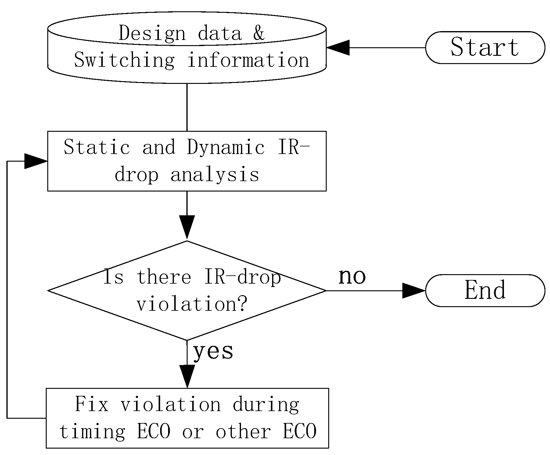
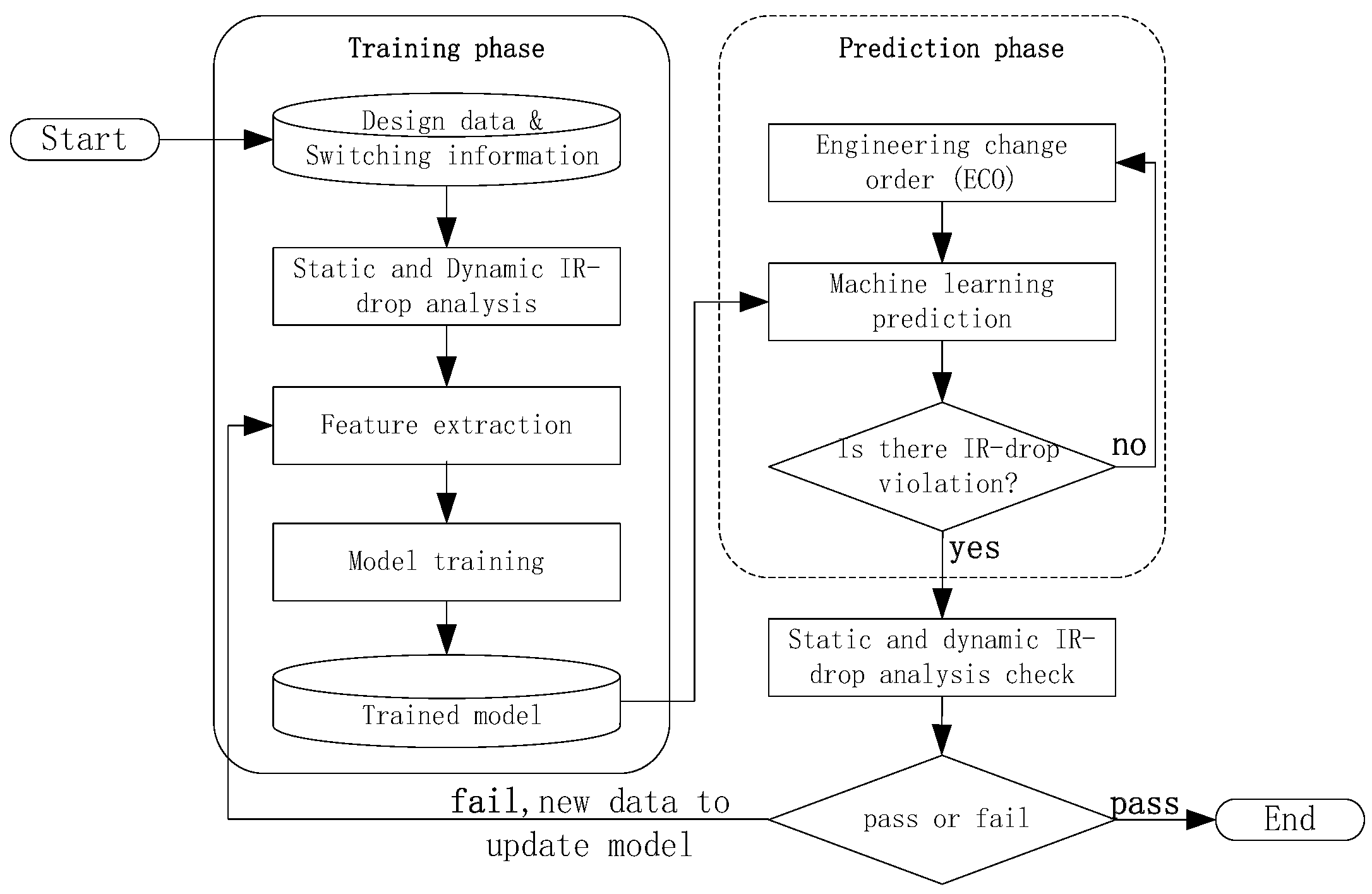
2.1. Proposed Flow
2.2. Nature Feature Extraction
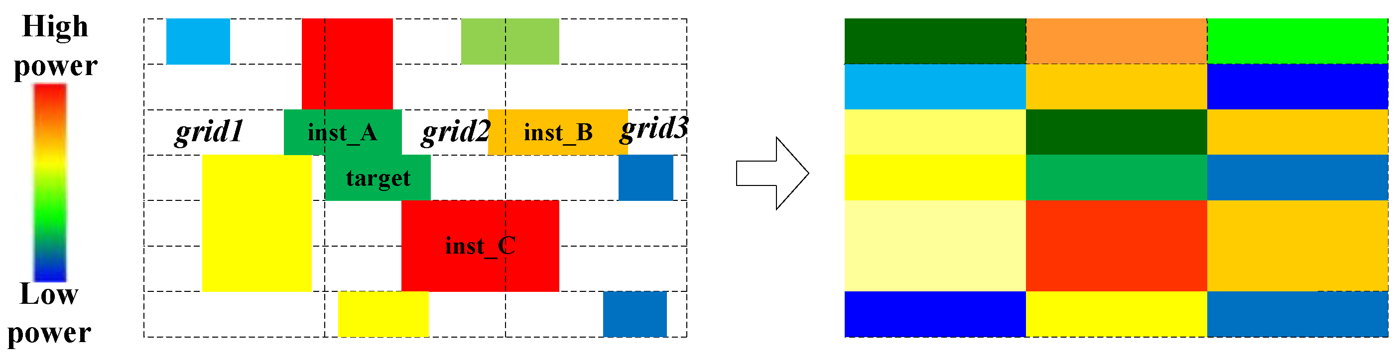
2.3. Neighboring Feature Construction
2.4. Design Matrix Construction
2.5. Training Model
3. Experiments Setup
4. Results
4.1. IR-Drop Prediction before ECO
4.2. IR-Drop Prediction after ECO
4.3. Runtime Comparison
5. Conclusions
Author Contributions
Funding
Institutional Review Board Statement
Informed Consent Statement
Data Availability Statement
Conflicts of Interest
References
- Shepard, K.L.; Narayanan, V. Noise in deep submicron digital design. In Proceedings of the International Conference on Computer Aided Design, San Jose, CA, USA, 9–13 November 1997; pp. 524–531. [Google Scholar]
- Tehranipoor, M.; Butler, K.M. Power supply noise: A survey on effects and research. IEEE Des. Test Comput. 2010, 2, 51–67. [Google Scholar] [CrossRef]
- Nithin, S.K.; Shanmugam, G.; Chandrasekar, S. Dynamic voltage (IR) drop analysis and design closure: Issues and challenges. In Proceedings of the IEEE International Symposium on Quality Electronic Design, San Jose, CA, USA, 15 April 2010; pp. 611–617. [Google Scholar]
- Holst, S.; Schneider, E.; Wen, X.; Kajihara, S.; Kochte, M.A. Timing-Accurate Estimation of IR-Drop Impact on Logic- and Clock-Paths during At-Speed Scan Test. In Proceedings of the IEEE Asian Test Symposium, Hiroshima, Japan, 21–24 November 2016; pp. 19–24. [Google Scholar]
- Pengcheng, H.; Shuming, C.; Jianjun, C. Simulation study of N-hit SET variation in differential cascade voltage switching logical circuits. Sci. China Inf. Sci. 2015, 58, 022401. [Google Scholar]
- Yamato, Y.; Yoneda, T.; Hatayama, K.; Inoue, M. A fast and accurate per-cell dynamic IR-drop estimation method for at-speed scan test pattern validation. In Proceedings of the IEEE International Test Conference, Anaheim, CA, USA, 5–8 November 2012; pp. 1–8. [Google Scholar]
- Chapelle, O.; Haffner, P.; Vapnik, V. Support vector machines for histogram-based image classification. IEEE Trans. Neural Netw. 1999, 5, 1055–1064. [Google Scholar] [CrossRef] [PubMed]
- Ye, F.; Firouzi, F.; Yang, Y.; Chakrabarty, K.; Tahoori, M.B. On-chip droop-induced circuit delay prediction based on support-vector machines. IEEE Trans. Comput. Aided Des. Integr. Circuits Syst. 2016, 4, 665–678. [Google Scholar] [CrossRef]
- Xie, Z.; Ren, H.; Khailany, B.; Sheng, Y.; Santosh, S.; Hu, J.; Chen, Y. PowerNet: Transferable dynamic IR drop estimation via maximum convolutional neural network. In Proceedings of the Asia and South Pacific Design Automation Conference, Beijing, China, 13–16 January 2020; pp. 13–18. [Google Scholar]
- Fang, Y.; Lin, H.; Su, M.; Li, C.; Fang, E.J. Machine-learning-based dynamic IR drop prediction for ECO. In Proceedings of the IEEE/ACM International Conference on Computer Aided Design, San Diego, CA, USA, 5–8 November 2018; pp. 1–7. [Google Scholar]
- Ho, C.; Kahng, A. IncPIRD: Fast learning-based prediction of incremental IR drop. In Proceedings of the IEEE/ACM International Conference on Computer Aided Design, Denver, CO, USA, 4–7 November 2019; pp. 1–8. [Google Scholar]
- Lin, H.; Fang, Y.; Liu, S.; Chen, J.X.; Fang, J.W. Automatic IR-drop ECO using machine learning. In Proceedings of the IEEE International Test Conference in Asia, Taipei, Taiwan, 23–25 September 2020; pp. 7–12. [Google Scholar]
- Pao, C.; Su, A.; Lee, Y. XGBIR: An XGBoost-based IR drop predictor for power delivery network. In Proceedings of the Design, Automation & Test in Europe Conference & Exhibition (DATE), Grenoble, France, 9–13 March 2020; pp. 1307–1310. [Google Scholar]
- Chen, T.; Guestrin, G. Xgboost: A scalable tree boosting system. In Proceedings of the 22nd ACM SIGKDD International Conference on Knowledge Discovery and Data Mining, San Francisco, CA, USA, 13–17 August 2016; pp. 785–794. [Google Scholar]
- Pu, Q.; Li, Y.; Zhang, H.; Yao, H.; Zhang, B.; Hou, B.; Li, L.; Zhao, Y.; Zhao, L. Screen efficiency comparisons of decision tree and neural network algorithms in machine learning assisted drug design. Sci. China Cemet. 2019, 62, 506–514. [Google Scholar] [CrossRef]
- Apache RedHawk User Manual. 2019. Available online: https://pdfcoffee.com/redhawk-pdf-free.html (accessed on 21 September 2021).


| Nature Features | Specifications |
|---|---|
| x, y | The x, y coordinate of an instance on layout design |
| CF | The code that represents the cell function of an instance |
| DS | The drive strength of an instance |
| VTT | The voltage threshold type of an instance |
| Rpu | The effective pull-up resistance of an instance |
| Rpd | The effective pull-down resistance of an instance |
| CL | The output load capacitance of an instance |
| Tog | The signal toggle rate of an instance |
| Il | The leakage current of an instance |
| SIA | The total of scaled dynamic current and leakage current of an instance |
| Ip | The peak current of an instance |
| Pl | The leakage power of an instance |
| SPi | The scaled internal power of an instance |
| SPs | The scaled switching power of an instance |
| SPA | The scaled total power of an instance |
| Circuit Design | DesignA | DesignB | |||
|---|---|---|---|---|---|
| Power Analysis Mode | Vectorless | VCD | Vectorless | VCD1 | VCD2 |
| Number of cell instance | 2.4 million | 2.4 million | 3.7 million | 3.7 million | 3.7 million |
| Mean IRD (mV) | 15.31 | 2.19 | 16.84 | 3.54 | 8.42 |
| Max IRD (mV) | 55.7 | 165.2 | 73.5 | 90.9 | 91.4 |
| Number of IRD violations | 0 | 576 | 9 | 28 | 173 |
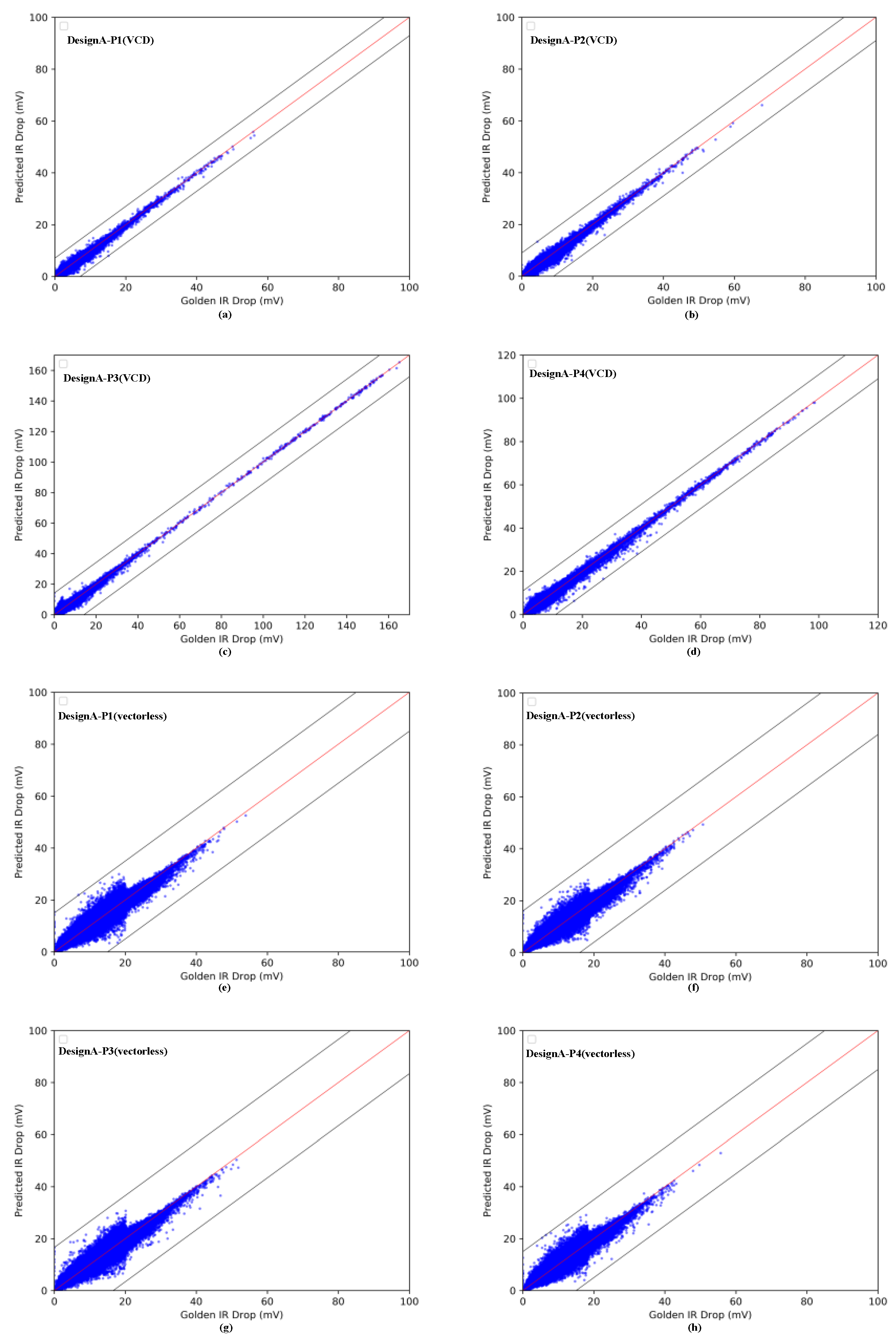
| Partitions | Power Analysis Mode | Inst Numbers | Mean IRD (mV) | CC | MAE (mV) | MaxE (mV) | RMSE |
|---|---|---|---|---|---|---|---|
| P1 | vectorless | 545,772 | 15.97 | 0.976 | 0.845 | 15.49 | 1.14 |
| VCD | 545,772 | 1.69 | 0.982 | 0.267 | 7.10 | 0.38 | |
| P2 | vectorless | 444,511 | 14.69 | 0.982 | 0.784 | 16.03 | 1.07 |
| VCD | 444,511 | 1.81 | 0.986 | 0.291 | 8.95 | 0.43 | |
| P3 | vectorless | 590,385 | 16.03 | 0.974 | 0.847 | 16.55 | 1.14 |
| VCD | 590,385 | 2.74 | 0.988 | 0.420 | 14.14 | 0.59 | |
| P4 | vectorless | 460,383 | 14.22 | 0.979 | 0.807 | 14.89 | 1.11 |
| VCD | 360,383 | 2.43 | 0.992 | 0.333 | 10.88 | 0.49 |
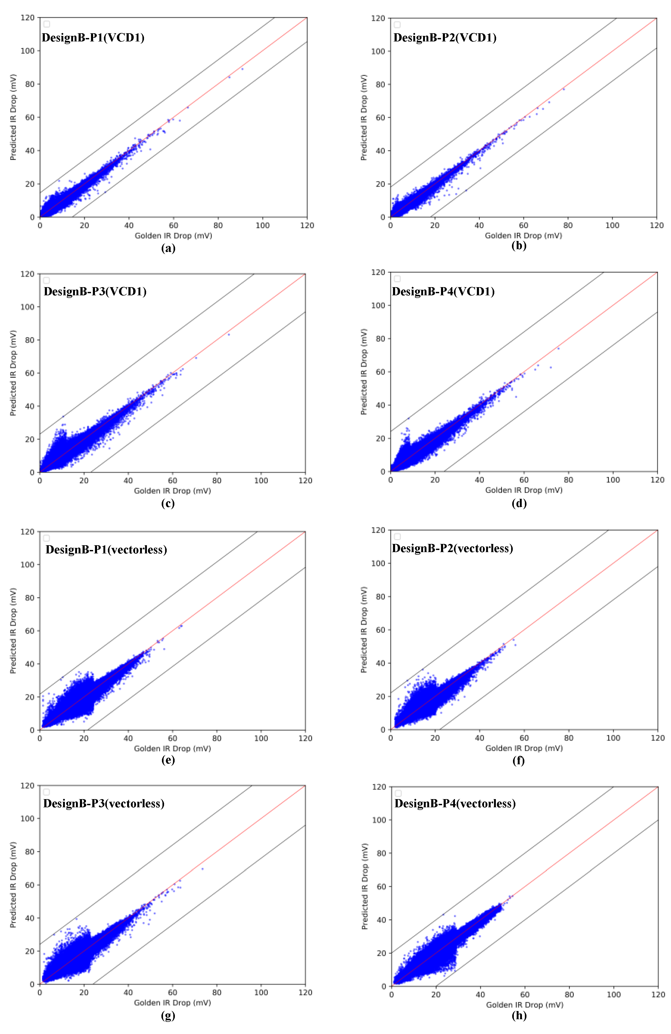
| Partitions | Power Analysis Mode | Inst Numbers | Mean IRD (mV) | CC | MAE (mV) | MaxE (mV) | RMSE |
|---|---|---|---|---|---|---|---|
| P1 | vectorless | 1,177,525 | 16.37 | 0.960 | 1260 | 21.53 | 1.67 |
| VCD1 | 1,177,525 | 1.70 | 0.976 | 0.312 | 14.29 | 0.48 | |
| VCD2 | 1,177,525 | 11.38 | 0.972 | 1116 | 21.44 | 1.57 | |
| P2 | vectorless | 947,562 | 14.13 | 0.960 | 1087 | 21.92 | 1.47 |
| VCD1 | 947,562 | 2.01 | 0.987 | 0.276 | 18.09 | 0.45 | |
| VCD2 | 947,562 | 4.13 | 0.961 | 0.777 | 22.17 | 1.17 | |
| P3 | vectorless | 782,721 | 16.81 | 0.963 | 1176 | 23.44 | 1.58 |
| VCD1 | 782,721 | 6.87 | 0.978 | 0.766 | 23.12 | 1.12 | |
| VCD2 | 782,721 | 9.63 | 0.980 | 1077 | 26.09 | 1.58 | |
| P4 | vectorless | 807,029 | 20.42 | 0.981 | 1092 | 19.81 | 1.47 |
| VCD1 | 807,029 | 4.87 | 0.974 | 0.652 | 23.79 | 0.96 | |
| VCD2 | 807,029 | 7.84 | 0.965 | 0.923 | 25.60 | 1.31 |
| Partitions | Power Analysis Mode | Inst Numbers | Mean IRD (mV) | CC | MAE (mV) | MaxE (mV) | RMSE |
|---|---|---|---|---|---|---|---|
| P1 | vectorless | 545,795 | 16.03 | 0.973 | 0.888 | 16.63 | 1.19 |
| VCD | 545,795 | 1.74 | 0.970 | 0.320 | 20.53 | 0.52 | |
| P2 | vectorless | 444,543 | 14.75 | 0.980 | 0.835 | 18.86 | 1.14 |
| VCD | 444,543 | 1.80 | 0.979 | 0.324 | 13.3 | 0.53 | |
| P3 | vectorless | 590,410 | 16.10 | 0.971 | 0.882 | 20.97 | 1.19 |
| VCD | 590,410 | 3.98 | 0.904 | 1189 | 22.45 | 1.88 | |
| P4 | vectorless | 460,400 | 14.12 | 0.975 | 0.887 | 16.30 | 1.20 |
| VCD | 460,400 | 2.08 | 0.901 | 0.882 | 20.02 | 0.98 |
| Partitions | Power Analysis Mode | Inst Numbers | Mean IRD (mV) | CC | MAE (mV) | MaxE (mV) | RMSE |
|---|---|---|---|---|---|---|---|
| P1 | vectorless | 1,185,523 | 16.25 | 0.882 | 2.347 | 32.91 | 2.99 |
| VCD1 | 1,185,523 | 1.69 | 0.962 | 0.379 | 31.04 | 0.66 | |
| VCD2 | 1,185,523 | 11.80 | 0.915 | 1955 | 35.96 | 2.88 | |
| P2 | vectorless | 959,577 | 14.15 | 0.908 | 2010 | 28.90 | 2.66 |
| VCD1 | 959,577 | 1.79 | 0.964 | 0.404 | 30.57 | 0.78 | |
| VCD2 | 959,577 | 4.46 | 0.945 | 0.887 | 34.47 | 1.36 | |
| P3 | vectorless | 812,582 | 16.90 | 0.910 | 2370 | 36.53 | 3.11 |
| VCD1 | 812,582 | 7.12 | 0.963 | 1091 | 37.70 | 1.68 | |
| VCD2 | 812,582 | 11.01 | 0.970 | 1700 | 39.91 | 3.08 | |
| P4 | vectorless | 829,071 | 20.63 | 0.929 | 2256 | 36.19 | 2.95 |
| VCD1 | 829,071 | 5.07 | 0.935 | 1049 | 30.80 | 1.73 | |
| VCD2 | 829,071 | 5.48 | 0.921 | 1485 | 39.50 | 1.49 |
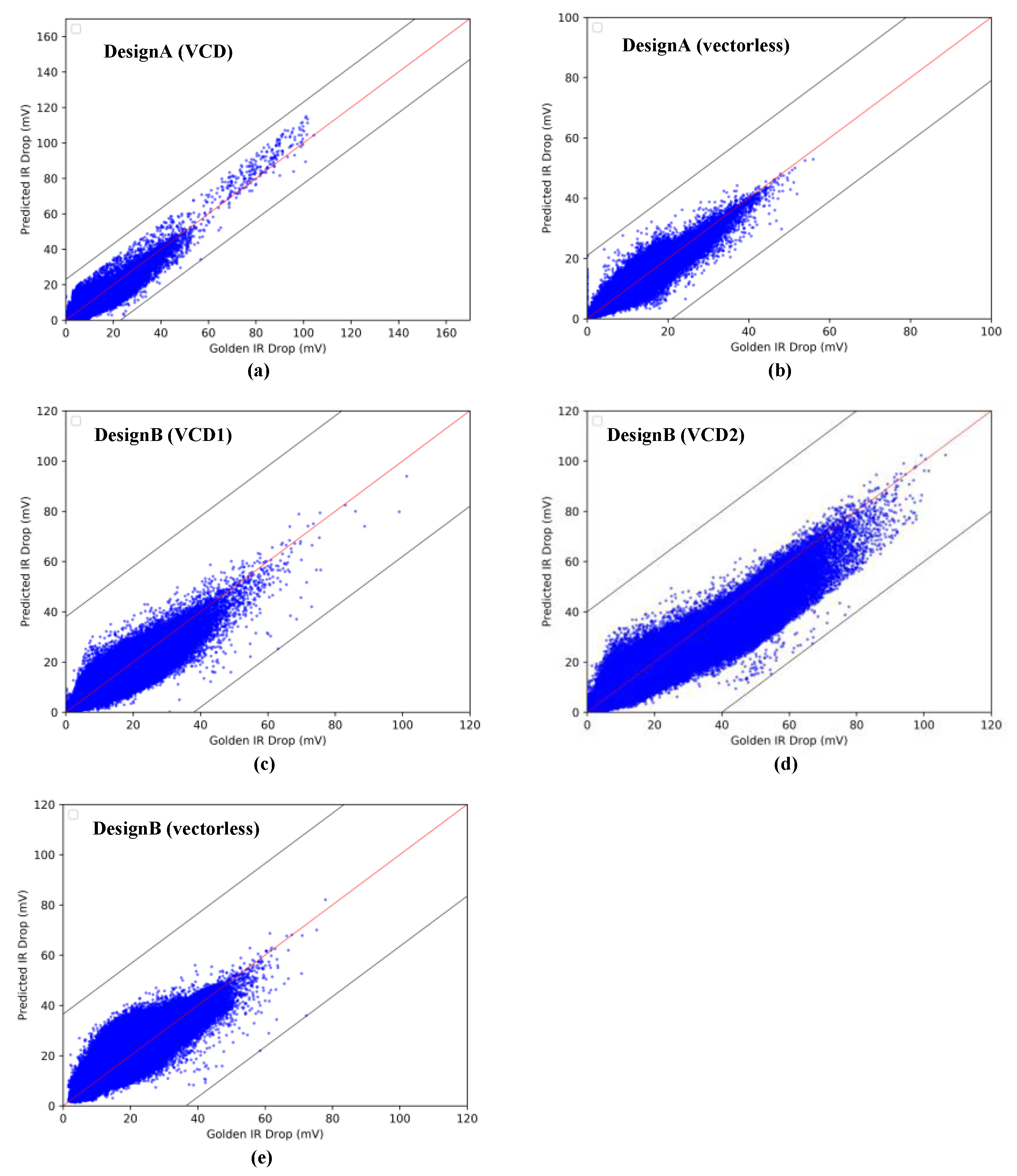
| Circuit Design | MAE (mV) | MaxE (mV) | CC | RMSE | TP | TN | FP | FN | Precision | Recall |
|---|---|---|---|---|---|---|---|---|---|---|
| DesignA (vectorlsess) | 0.875 | 20.97 | 0.975 | 1.181 | 0 | 2041148 | 0 | 0 | NAN | NAN |
| DesignA (VCD) | 0.643 | 22.45 | 0.925 | 1.209 | 246 | 2040884 | 13 | 5 | 0.950 | 0.980 |
| DesignB (vectorlsess) | 2.247 | 36.53 | 0.916 | 2.925 | 13 | 3786717 | 2 | 21 | 0.867 | 0.382 |
| DesignB (VCD1) | 0.739 | 37.70 | 0.954 | 1.410 | 27 | 3786678 | 7 | 41 | 0.794 | 0.397 |
| DesignB (VCD2) | 1.526 | 39.91 | 0.952 | 2.488 | 2137 | 3781511 | 143 | 2962 | 0.937 | 0.419 |
| Circuit Design | DesignA (Vectorless) | DesignA (VCD) | DesignB (Vectorless) | DesignB (VCD1) | DesignB (VCD2) |
|---|---|---|---|---|---|
| Constructing training matrix | 23 min 22 s | 21 min 49 s | 24 min 7 s | 22 min 31 s | 22 min 43 s |
| Training | 30 min 11 s | 30 min 7 s | 30 min 12 s | 30 min 8 s | 30 min 9 s |
| Constructing predicting matrix | 1 h 11 min | 1 h 9 min | 1 h 36 min | 1 h 27 min | 1 h 27 min |
| Predicting | 31 s | 30 s | 39 s | 38 s | 38 s |
| IRD analysis by Redhawk | 5 h 41 min | 5 h 35 min | 6 h 57 min | 6 h 34 min | 6 h 44 min |
Publisher’s Note: MDPI stays neutral with regard to jurisdictional claims in published maps and institutional affiliations. |
© 2021 by the authors. Licensee MDPI, Basel, Switzerland. This article is an open access article distributed under the terms and conditions of the Creative Commons Attribution (CC BY) license (https://creativecommons.org/licenses/by/4.0/).
Share and Cite
Huang, P.; Ma, C.; Wu, Z. Fast Dynamic IR-Drop Prediction Using Machine Learning in Bulk FinFET Technologies. Symmetry 2021, 13, 1807. https://doi.org/10.3390/sym13101807
Huang P, Ma C, Wu Z. Fast Dynamic IR-Drop Prediction Using Machine Learning in Bulk FinFET Technologies. Symmetry. 2021; 13(10):1807. https://doi.org/10.3390/sym13101807
Chicago/Turabian StyleHuang, Pengcheng, Chiyuan Ma, and Zhenyu Wu. 2021. "Fast Dynamic IR-Drop Prediction Using Machine Learning in Bulk FinFET Technologies" Symmetry 13, no. 10: 1807. https://doi.org/10.3390/sym13101807
APA StyleHuang, P., Ma, C., & Wu, Z. (2021). Fast Dynamic IR-Drop Prediction Using Machine Learning in Bulk FinFET Technologies. Symmetry, 13(10), 1807. https://doi.org/10.3390/sym13101807