Optimizing the Tolerance for the Products with Multi-Dimensional Chains via Simulated Annealing

Abstract

The assembly is the last process of controlling the product quality during manufacturing. The installation guidance should provide the appropriate assembly information, e.g., to specify the components in each product. The installation guidance with low quality results in rework or the resource waste from the failure products. This article extends the dimensional chain assembly problem proposed by Tsung et al. to consider the multiple dimensional chains in the product. Since there are multiple dimensional chains in a product, the installation guidance should consider inseparability and acceptability as computing the installation guidance. The inseparability means that the qualities of all dimensional chains in the part should be evaluated together without separation, while the acceptability stands for that the size of each product should be satisfied with the specification. The simulated annealing (SA) algorithm is applied to design the assembly guidance optimizer named as $AG{O}_{MDC}$ to compute the assembly guidance in the dimensional chain assembly problem with multiple dimensional chains. Since SA has high performance in searching neighbor solutions, the proposed approach could converge rapidly. Thus, proposed $AG{O}_{MDC}$ could be applied in real-world application for the implementation consideration. The simulations consist of two parts: the feasibility evaluation and the algorithm configuration discussion. The first part is to verify the inseparability and acceptability that are the hard constraints of the assembly problem for the proposed $AG{O}_{MDC}$, and the second one is to analyze the algorithm configurations to calculate the assembly guidance with 80% quality. The simulation results show that the inseparability and acceptability are achieved, while the proposed $AG{O}_{MDC}$ only requires more than two seconds to derive the results. Moreover, the recommended algorithm configurations are derived for evaluate the required running time and product quality. The configurations with product quality 80% are that the temperature descent rate is 0.9, the initial temperature is larger than 1000, and the iteration recommended function is derived based on the problem scale. The proposed $AG{O}_{MDC}$ not only helps the company to save the time of rework and prevent the resource waste of the failure products, but is also valuable for the automatic assembly in scheduling the assembly processes.

1. Introduction

Owing to information and communications technologies (ICT), Industry 4.0 becomes the popular topic in manufacturing, information science, and industrial management [1,2]. The major technologies that are applied to realize Industry 4.0 include Internet of Things to collect data [3,4,5], cloud in storing and preparing data [6,7,8], and artificial intelligence [9,10] and data analysis [11,12] for extracting the knowledge from data. So, the producing managers could use the derived knowledge to enhance manufacturing efficiency.

Assembly is the last step of manufacturing, and it is also the last process of controlling the production quality [13]. After receiving some components and the installation guidance, the assemblers pick up the specific components and assemble the selected components together to the products or modules. 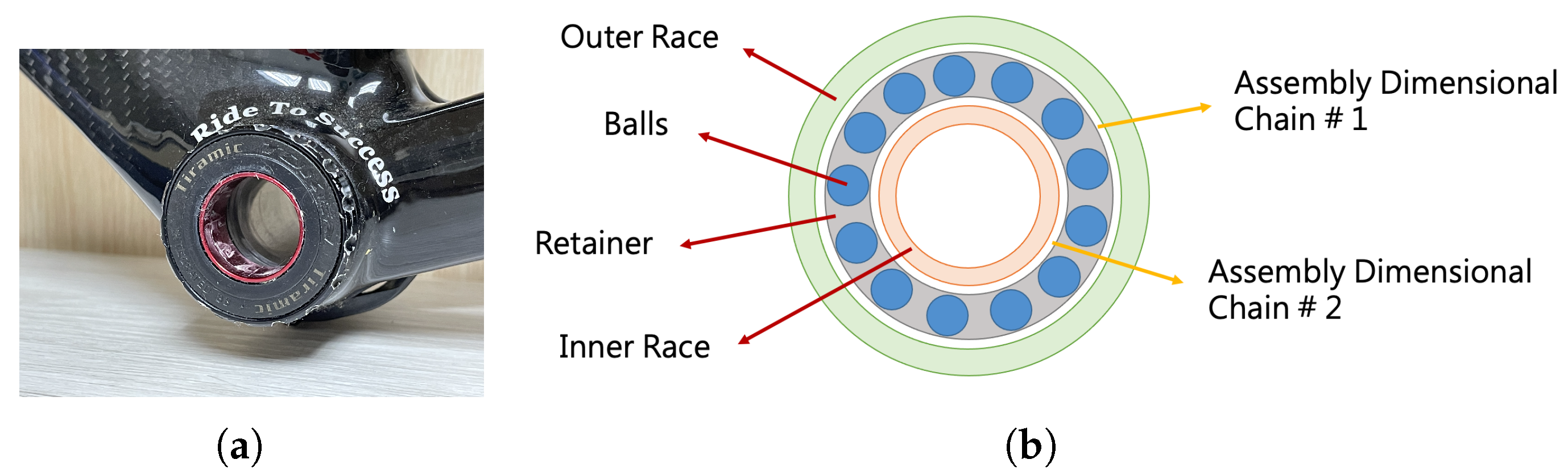The real size of each component would be different with that of the design size, so the tolerance is allowed in manufacturing [14]. However, the tolerance determines the size of the products, and that is the product quality. We use the bearing shown in Figure 1 as the example to explain the product quality. The bearing should be installed in the bottom bracket of a bike, as shown in Figure 1a, and the composition diagram is illustrated in Figure 1b. Each bearing consists of one outer race, some balls, one retainer, and one inner race. Since the balls and retainer should be pre-installed, we treat the balls and retainer are assembled as one module. So, the assembler would pick up one outer race, one retainer, and one inner race to assemble a bearing. The bearings have two surfaces to touch bottom bracket of a bike and the crank axles. The bottom bracket touches the outer race, while the crank axles touch the inner race. The quality of bearings is determined by the sizes of outer race and inner race, and they are assembled with the retainer module. The selection of the components determines the final sizes of the products. Therefore, the assembly process would be the last step in controlling the product quality.

If the assemblers arbitrarily pick up the components and assemble them together, the products may be out of the specification. Thus, the defect products require rework to fix the defect, and the products with poor quality will be abandoned. Inappropriate assembly process will increase the manufacturing cost. To increase the product quality and decrease the manufacturing cost, analyzing the dimensional chain to guarantee the size of each product [15,16] and computing the installation guidance to assemble appropriate components together [16,17] are feasible solutions. The dimensional chain is analyzed before manufacturing process and the installation guidance is calculated after manufacturing. Therefore, calculating the installation guidance is more appropriate than analyzing the dimensional chain from the perspective of the implementation.

From the above example, the product quality is determined by the components selected by assemblers. Quality control officers have to measure the component sizes one by one in the traditional manufacturing, and this manner requires huge cost. The ICT based services help measurers to collect the component sizes automatically [18,19], and the cost is reduced. Therefore, collecting all sizes of components becomes available and requires less cost than in traditional manufacturing.

Tsung et al. formulated the calculation of installation guidance as the dimensional chain assembly (DCA) problem, and proposed the assembly guidance optimizer (AGO) to calculate the installation guidance [17]. The DCA problem proposed by Tsung et al. considers the product that consists of 11 parts with one-dimensional chain. However, in the real-world instance, most products consist of some dimensional chains, but this property is not considered in the DCA. Considering that the bearing as shown in Figure 1, there are two dimensional chains, and they cross on the part retainer. Replacing the retainer to another one would results in different quality of both dimensional chains. Therefore, we modify the DCA problem to the dimensional chain assembly, with multiple dimensional chains problem named by $DC{A}_{MDC}$ for involving the concept of multiple dimensional chains in this article. The major difference between single dimensional chain and multiple dimensional chains is to consider the inseparability of dimensional chains. Multiple dimensional chains may cross on one part, so replacing the part results in the different quality of all corresponding dimensional chains. Therefore, the inseparability of multiple dimensional chains should be taken into account when evaluating the solution quality.

There is exactly one-dimensional chain in the DCA problem, so the solution quality is defined by the size of the dimensional chain. We extend this idea from the DCA problem to the $DC{A}_{MDC}$ problem, but it fails. The solution quality comes from multiple dimensional chains in the $DC{A}_{MDC}$ problem, so we have to normalize the sizes of all dimensional chains to the solution quality. According to the min-max theorem [20,21], minimizing the worst quality increases the solution quality for the whole solution. Thus, we consider the worse quality from all dimensional chains as the solution quality, so the inseparability could be satisfied.

Except for the inseparability of multiple dimensional chains, the solution feasibility is another critical issue. All product sizes are specified in the product design phase, and the designer would list the size information for components and sizes in the specification. The feasibility indicates that the quality of each dimensional chain should fit the requirements listed in the specification. To achieve the solution feasibility, we extend the AGO algorithm proposed by Tsung et al. [17] to the Assembly Guidance Optimizer with Multiple Dimensional Chains denoted by $AG{O}_{MDC}$ to solve the $DC{A}_{MDC}$ problem. The $AG{O}_{MDC}$ algorithm is the application of the simulated annealing (SA) [22,23]. We proposed a new solution format, the local search algorithm, and the equation of calculating the maximum iteration to realize the solution with the approximation ratio 0.8.

In the simulation, we receive a batch of component sizes for assembling bearings from the assembly line, and the mission is to calculate the assembly guidance that the inseparability and the feasibility are satisfied. To increase the diversity of the dataset, we analyze the received size data to design the case generator, and we can generate synthetic data to cover more instance properties. From the first simulation results, the solution derived from the proposed $AG{O}_{MDC}$ reaches both the inseparability and the feasibility. Moreover, $AG{O}_{MDC}$ consume 562.6 milliseconds to derive the solution, so the running time is acceptable. The first simulation indicates that computing the feasible solutions by the proposed $AG{O}_{MDC}$ is not difficult, and we organize the second simulation to analyze the algorithm configuration for ensuring the solutions with 80% quality. Therefore, the assembly manager could rapidly determine the algorithm configuration based on the problem properties, and the product quality is also guaranteed. From the simulation results, the configurations with product quality 80% are that the temperature descent rate is 0.9, the initial temperature is larger than 1000, and the iteration recommended function is derived based on the problem scale.

The major contributions of this article include: (1) formulating the $DC{A}_{MDC}$ as the optimization problem for complex product assembly, (2) applying the SA to compute the installation guidance, and (3) proposing the algorithm configuration for the assembly manager for adjusting the proposed algorithm to compute the installation guidance with the guarantee of 80% product quality.

In the following article, some related works are discussed in Section 2. The $DC{A}_{MDC}$ problem is defined in Section 3, and the example of assembling bearings would be given to explain the $DC{A}_{MDC}$ problem. In Section 4, the main algorithm of $AG{O}_{MDC}$ is present, and the details of the solution format and the solution quality are stated simultaneously. The simulation results and the application of $AG{O}_{MDC}$ algorithm is discussed in Section 5, and the conclusion is in Section 6.

2. Related Works

The tolerance calculation helps to increase the product quality. Increasing purchasing provides high motivation in statistical tolerance calculations in Europe [24,25]. Moreover, in Europe, feature factories target at the term “Zero Defect Manufacturing” and set it as the milestone in 2020 roadmap [26]. We all know the importance of the tolerance calculation, but however, only a few companies apply the tolerance calculation in manufacturing in German from the analysis of Walter et al. [27]. In the past decade, collect all sizes of each component is difficult, but it is realized easier currently due to the publication of the ICT applications, such as Internet of Things [28] and cloud computing [29]. So, more companies would like to consider the tolerance calculation, since the difficulty of data collection is eased.

In the assembly line, the assemblers receive an installation guidance, and they follow the instructions listed in the installation guidance to pick up the specify components and assemble the selected components together. The goal of the assembly problem is to determine the installation guidance to specify the components in a product such that the product quality fits the requirements of the specification. There are two manners to determine the installation guidance, and they are discussed as follows.

• The dimension chain analysis in the product design phase [15,16]: the properties of components are designed, including the ideal component size, the tolerance, and the size of touch surface. Then, the dimensional chain analysis is applied to estimate the product size. If the product size is unacceptable, the designer should modify the components until the product size is acceptable.
• The installation guidance analysis [17]: the installation guidance analysis analyzes the component sizes and determines the installation guidance to specific the components in each product. The major difference between the above manners is the analysis timing.

Above approaches could provide installation guidance, but the dimensional chain analysis takes place in the design phase, while the installation guidance analysis is executed after the manufacturing processes. The dimensional chain analysis provides precise prediction in product quality only if the quality of manufacturing processes is guaranteed. The installation guidance analysis considers real size information, and thus, the installation guidance analysis provides the installation guidance based on the real sizes of the components. Therefore, this article considers the installation guidance analysis.

The installation guidance analysis could be formulated as the optimization problem, and some heuristic algorithms could be applied to determine the installation guidance. Kim et al. used taboo search and SA to determine the swap of the assembly process to minimize mean tardiness [30]. Ge et al. proposed the homogeneous Markov chain of reassembly process for the assembly process of remanufactured crankshaft [31], and the term “reassembly” has been applied to enhance the product quality. Rausch et al. focused on easing the assembly rework to enhance the assembly efficiency, and the authors applied Monte Carlo simulation to identify potential misalignments [32]. Homri et al. consider the parts’ form defects to the over-constrained assemblies [33]. Morse et al. mentioned that the variability should be allowed and controlled to maintain the product function [34]. Tsung et al. consider the SA to compute the installation guidance to maximize the quality for all products [17].

The $DC{A}_{MDC}$ problem differs from the DCA problem that is proposed by Tsung et al. [17] in terms of the number of dimensional chains. The DCA problem consists of a one-dimensional chain, and the $DC{A}_{MDC}$ problem has multiple dimensional chains. In the $DC{A}_{MDC}$ problem, the multi-objective decision analysis [35,36,37] should be considered to transform multiple objectives to single objective. There are some techniques of deriving the single objective, and we consider the score normalization in the $DC{A}_{MDC}$ problem. For the perspective of the feasibility, the size of each dimensional chain should be satisfied with the specification. Therefore, the importance of each dimensional chain is equal, and the score normalization is feasible in the $DC{A}_{MDC}$ problem.

3. The Dimensional Chain Assembly with Multiple Dimensional Chains Problem

Before formulating the problem, some preliminaries are necessary, including the target of assembly, the installation guidance, the dimensional chains, and the symbolic system. Thus, the preliminaries are given in Section 3.1, the problem definition is in Section 3.2, and an example is provided to explain the problem and the goal in Section 3.3.

3.1. Preliminary

• Background of Assembly: Suppose the target product consists of $\left|P\right|$ parts. As the example shown in Figure 1 demonstrates, the bearings have three parts, i.e., $\left|P\right|=3$, and they are outer race, retainer module, and inner race. The assembler picks up $\left|P\right|$ components where one per part and assembles $\left|P\right|$ selected components together to produce one product. In Figure 1, the assembler picks up three components—one outer race, one retainer module, and one inner race and then assembles them together. Given $\left|P\right|$ parts and that each part has $\left|T\right|$ components, the number of components that are delivered to the entrance of the assemble line is $\left|T\right|\times \left|P\right|$. So, the assembler selects $\left|P\right|$ components to produce one product and repeats $\left|T\right|$ times to finish $\left|T\right|$ products in total.
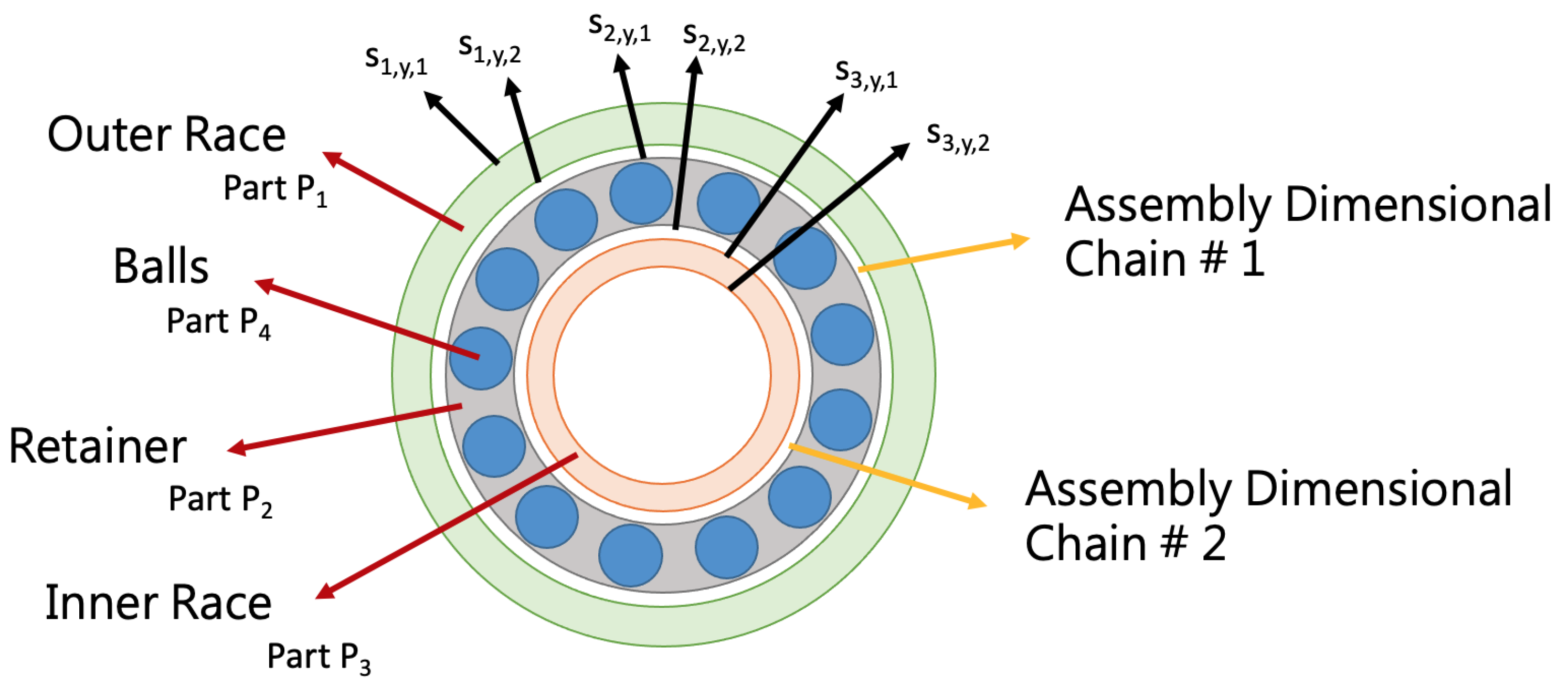
• Component Sizes: The label $co{m}_{j,y}$ indicates y-th component of j-th part, where $0\le y<\left|T\right|$ and $0\le j<\left|P\right|$. The component $co{m}_{j,y}$ has several component sizes, and $s_{j,y,z}$ is applied to represent the z-th component size of $co{m}_{j,y}$. For example, the outer race in Figure 1b has two component sizes, and they are the outside diameter and inside diameter.
• Multiple dimensional chains: The major difference between DCA proposed by Tsung et al. [17] and $DC{A}_{MDC}$ is the number of dimensional chains in a product. In the DCA, the product has exactly one-dimensional chain, e.g., crankshafts, but there are several dimensional chains in a product for $DC{A}_{MDC}$, e.g., bearings. Suppose each product consists of $\left|C\right|$ dimensional chains in $DC{A}_{MDC}$; it means that each product has $\left|C\right|$ product sizes. Thus, $\left|C\right|=2$ in Figure 1b. Chain number one consists of outer race and retainer module, while chain number two consists of retainer module and inner race. Moreover, one part may belong to several chains. The retainer module shown in Figure 1 belongs to both dimensional chains.
• Product tolerance: Since each product has $\left|C\right|$ dimensional chains in $DC{A}_{MDC}$, there are $\left|C\right|$ product sizes in each product. According to the assembly position in the dimensional chain k, each component $co{m}_{j,y}$ has three statuses: (1) $co{m}_{j,y}$ contains other components, (2) $co{m}_{j,y}$ is in other components, and (3) $co{m}_{j,y}$ does not belong to the dimensional chain k. For the chain number one in Figure 1b, the retainer module is in the outer race, and the inner race is not in the chain number one. After assembling a product, $\left|C\right|$ product sizes are derived, and the label $p{s}_k^i$ represents the product size for k-th chain in i-th product. Thus, the tolerance for the dimensional chain is the gap between $p{s}_k^i$ and the ideal product size.
• Product specification: The product specification includes three values—the lower bound of tolerance, the central value, and the upper bound of tolerance for each dimensional chain. The central value is the ideal product size, while the product specification specifies the ranges of the acceptable products for the dimensional chain. Since the cutting process may result in the tolerance, the product designer provides the CAD size for each part with a specific range. Here, we assume that the sizes of all components are satisfied with the range requirement. The out-of-range components could be fixed by the rework, so the assumption is rational.
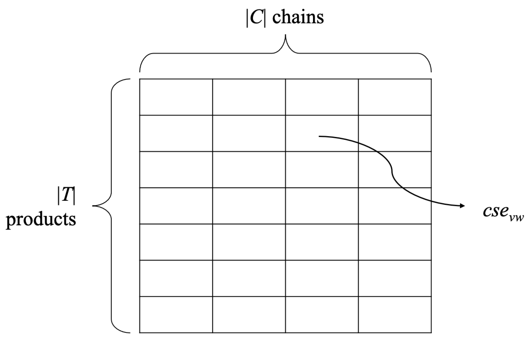
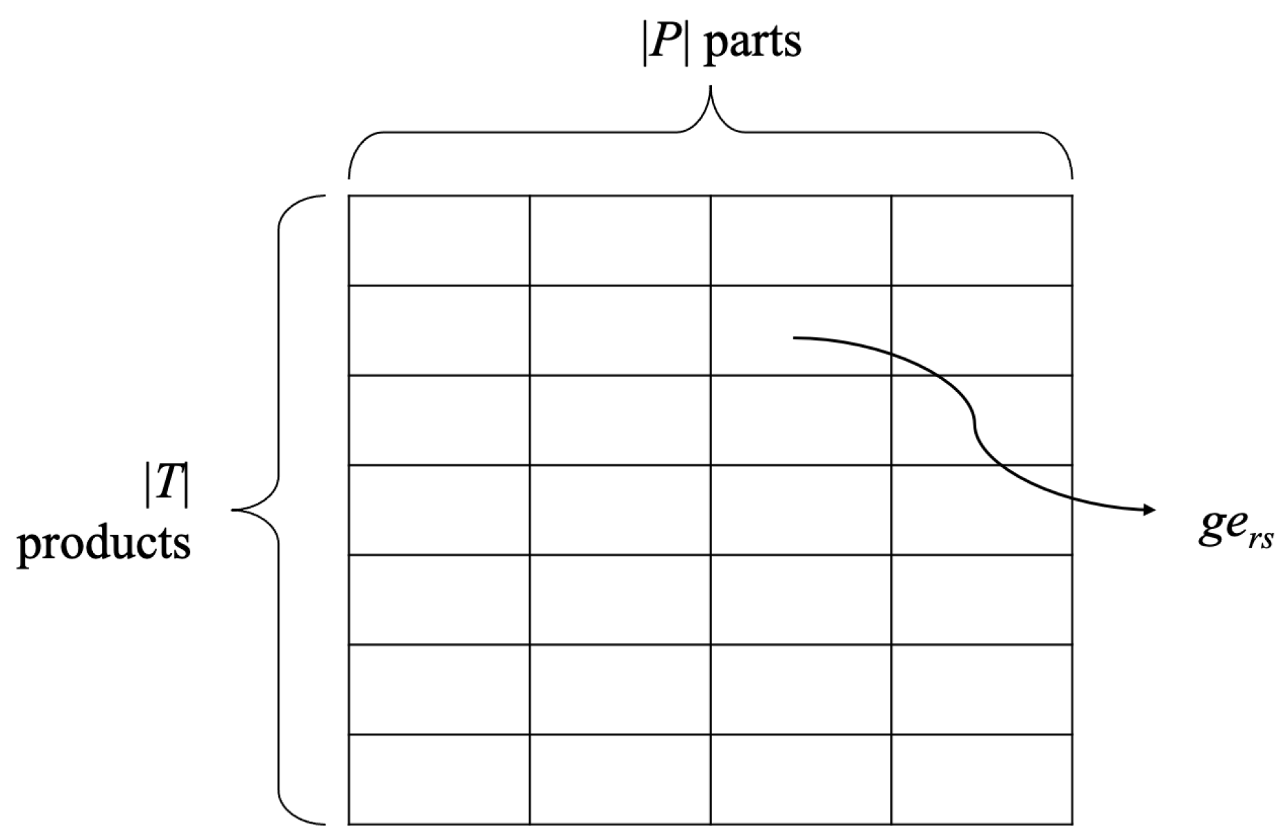
• The installation guidance: The installation guidance specifies the components of each product, so the assemblers could follow the guidance to assemble products. Since each product consists of $\left|P\right|$ components, a two-dimensional structure ($\left|T\right|$ by $\left|P\right|$) is used to represent the installation guidance for assembling $\left|T\right|$ products, as illustrated in Figure 2. The element $g{e}_{rs}$ in the installation guidance represents the component index for r-th product with s-th part, so each row indicates the components of the product. The details of the installation guidance will be provided when introducing the proposed solution in Section 4.2.

3.2. Definition of $DC{A}_{MDC}$

An instance of $DC{A}_{MDC}$ consists of $\left|T\right|\times \left|P\right|$ components and $\left|C\right|$ dimensional chains, and $\left|T\right|$ products will be generated eventually. The y-th component in j-th part $co{m}_{j,y}$ has several component sizes, and z-th component size is $s_{j,y,z}$. Each product has $\left|C\right|$ product sizes, and each product size $p{s}_k^i$ matches to the corresponding dimensional chain. To calculate $p{s}_k^i$, the decision variable $x_{j,y,z}$ as shown in Equation (1) is applied to formulate the relationship between components in each dimensional chain. Consider that two components $co{m}_{j,y}$ and $co{m}_{j^{\prime },y}$ where $j\ne j^{\prime }$ with component sizes $s_{j,y,z}$ and $s_{j^{\prime },y,z}$ for the same dimensional chain, respectively. If $co{m}_{j^{\prime },y}$ contains $co{m}_{j,y}$ which means $co{m}_{j,y}$ is in $co{m}_{j^{\prime },y}$, the size of the assemble surface between $co{m}_{j,y}$ and $co{m}_{j^{\prime },y}$ is $(s_{j^{\prime },y,z}-s_{j,y,z})$ that is identical to $(s_{j^{\prime },y,z}\times 1)+(s_{j,y,z}\times -1)$. The decision variables of $co{m}_{j,y}$ and $co{m}_{j^{\prime },y}$ are 1 and −1, respectively.

$$x_{j,y,z}=\left\{\begin{array}{ccc}\hfill -1& & \mathrm{if} co{m}_{j,y}\mathrm{is}\mathrm{assembled}\mathrm{in}\mathrm{other}\mathrm{part}\hfill \\ \hfill 0& & \mathrm{if} co{m}_{j,y}\mathrm{does}\mathrm{not}\mathrm{infolve}\mathrm{in}\mathrm{dimensional}\mathrm{chain}\hfill \\ \hfill 1& & \mathrm{if} co{m}_{j,y}\mathrm{contains}\mathrm{other}\mathrm{components}.\hfill \end{array}\right.$$

(1)

Therefore, the product size $p{s}_k^i$ for chain k could be derived in Equation (2). The idea of calculation is to sum up the product of component sizes and the corresponding decision variables for all possible permutations.

$$p{s}_k^i=\sum _{\forall j}\sum _{\forall y}\sum _{{\forall }_z}{s}_{j,y,z}\times x_{j,y,z}.$$

(2)

Given an instance of $DC{A}_{MDC}$ and the product specification with the lower bound $l{b}_k$, the central value $c{v}_k$, and the upper bound $u{b}_k$ for chain k, where $l{b}_k\le 0$, $c{v}_k\in R$, and $0\le u{b}_k$, the goal of $DC{A}_{MDC}$ is to calculate the installation guidance, so that each $p{s}_k^i$ is within the lower bound of tolerance and the upper bound of tolerance from the specification for all dimensional chains. A feasible solution of $DC{A}_{MDC}$ should be satisfied with the inseparability and acceptability:

• Inseparability: The multi-dimensional chains mean that the product consists of several dimensional chains, and some dimensional chains may cross on one part. Thus, the part that is crossed by some dimensional chains cannot be separated as evaluating the solution quality.
• Acceptability: The acceptability means that the tolerance of each dimensional chain must be satisfied with the specification. From the product specification, the range of acceptable tolerance is illustrated in Figure 3. The red line indicates the feasible tolerance range that the product sizes should fall into. The optimal solution indicates that $p{s}_k^i$ is identical to $c{v}_k$ for each i.

Computing the solution with inseparability and acceptability is the goal of solving $DC{A}_{MDC}$. However, this is insufficient for the perspective of implementation, because the assembly managers have no idea to extend the solution to other $DC{A}_{MDC}$ problems. Therefore, the other objective of this article is to provide the approach to compute the solution with 80% quality.

3.3. A Case Study of Bearing Assembly

Given the bearing assembly line, the composition diagram is shown in Figure 4. Suppose that the balls are preinstalled in the retainer, and the balls and the retainer could be treated as the retainer module. The assembly process includes three parts, i.e., $\left|P\right|=3$, the outer race, the retainer module, and the inner race with labels $j=1,2,3$, respectively. Each part has two sizes in this example where the outside size is marked as number one, while inside size is number two. Therefore, the outer race has outside diameter $s_{1,y,1}$ and inside diameter $s_{1,y,2}$; the retainer module has outside diameter $s_{2,y,1}$ and inside diameter $s_{2,y,2}$; the inner race has outside diameter $s_{3,y,1}$ and inside diameter $s_{3,y,2}$ for y-th componment. The outer race and retainer module are involved in the chain number one while chain number two has the retainer module and inner race. Equation (3) is derived by expanding Equation (2). Since only component sizes $s_{1,y,2}$ and $s_{2,y,1}$ are in dimensional chain number one, e.g., $k=1$, the values of $x_{1,y,2}$ and $x_{2,y,1}$ are non zero. Thus, the product sizes of i-th product is calculated by Equations (4) and (5) for chain number two.

$$\begin{array}{cc}\hfill p{s}_k^i=& s_{1,y,1}\times x_{1,y,1}+s_{1,y,2}\times x_{1,y,2}+s_{2,y,1}\times x_{2,y,1}+s_{2,y,2}\times x_{2,y,2}+\hfill \\ \hfill & s_{3,y,1}\times x_{3,y,1}+s_{3,y,2}\times x_{3,y,2}\hfill \end{array}$$

(3)

$$p{s}_1^i=s_{1,y,2}\times x_{1,y,2}+s_{2,y,1}\times x_{2,y,1}$$

(4)

$$p{s}_2^i=s_{2,y,2}\times x_{2,y,2}+s_{3,y,1}\times x_{3,y,1}$$

(5)

Considering that the assembly line receives 12 components that four for part number one, four for part number 2, and four for part number 3, as shown in

Table 1. The size information for each component.

Workpiece	${wp}_{\mathit{j}1}$	${wp}_{\mathit{j}2}$	${wp}_{\mathit{j}3}$	${wp}_{\mathit{j}4}$
$(s_{1,y,1},s_{1,y,2})$	(12.5, 10.08)	(12.5, 10.2)	(12.5, 10.14)	(12.5, 10.1)
$(s_{2,y,1},s_{2,y,2})$	(9.97, 7.17)	(9.86, 7.2)	(9.9, 7.18)	(9.9, 7.15)
$(s_{3,y,1},s_{3,y,2})$	(7, 5)	(6.8, 5)	(6.87, 5)	(6.9, 5)

, the label $w{p}_{jx}$ indicates the x-th workpiece for j-th part. The objective is to assemble four bearings with the specification listed in

Table 2. The specification of target bearings of the example listed in Table 1.

	Chain Number One	Chain Number Two
$l{b}_k$	−0.05	−0.15
$c{v}_k$	0.2	0.25
$u{b}_k$	0.2	0.18

. In other words, the sizes of the acceptable bearing should be within 0.15 and 0.4 for chain number one, and 0.1 and 0.43 for chain number two.

Suppose that the installation guidance with four bearings is ($w{p}_{11}$, $w{p}_{21}$, $w{p}_{31}$), ($w{p}_{12}$, $w{p}_{22}$, $w{p}_{32}$), ($w{p}_{13}$, $w{p}_{23}$, $w{p}_{33}$), and ($w{p}_{14}$, $w{p}_{24}$, $w{p}_{34}$). The guidance indicates that the first product consists of three components, and they are $w{p}_{11}$, $w{p}_{21}$, and $w{p}_{31}$ from part 1, 2, and 3 respectively. The gaps between $p{s}_k^i$ and $c{v}_k$ are $(0.11,0.17)$, $(0.34,0.4)$, $(0.24,0.31)$, and $(0.2,0.25)$ for (chain number one, chain number two), respectively. For convenience, we use ${\Delta }_k^i$ to represent the gap that is the tolerance between $p{s}_k^i$ and $c{v}_k$. The first bearing is unacceptable because the sizes are 0.11 and 0.17 for chain number one and chain number two, but however the acceptable specification should be within ($0.15,0.4$) and ($0.1,0.43$). The size of chain number two of the first bearing is smaller than the lower bound of the specification, so the first bearing is unacceptable. Eventually, the solution is infeasible.

4. Assembly Guidance Optimizer with Multiple Dimensional Chains

The $DC{A}_{MDC}$ is a permutation problem. For the perspective of permutation, the goal is to find out a permutation that the installation guidance is satisfied with the inseparability and acceptability, as shown in Section 3.2. The exhaustive search [38] could obtain the optimal solution with minimum $p{s}_k^i$, but the time complexity is increased by the number of products, i.e., $\left|T\right|$, and the assembly complexity, i.e., $\left|P\right|$. Computing the optimal would pay more computation cost, so the near-optimal solutions are more appropriate than the optimal solution.

Several heuristic algorithms are proposed to compute the near optimal solution in large-scale search space; for example, genetic algorithm (GA) [39], Tabu search [40], ant colony optimization [41], SA [42,43], and flower pollination algorithm [44]. The heuristic algorithms could be classified into single solution-based (SS) approach, e.g., Tabu search and SA, and multi-solution-based (MS) approach, e.g., GA, ant colony optimization, and flower pollination algorithm. The major difference is that the MS approaches estimate several solutions in an iteration and only one solution is processed in the SS solution. In an iteration, MS approaches require a longer processing time than that of SS approaches, and MS approaches provide wider search than SS approaches. Theoretically, the MS approaches output the solutions with better quality than SS approaches, because of the search width. The MS approaches provide higher solution quality than that of the SS approaches, but the quality of output solution is not so stable as that of the SS approaches. The MS approaches parallelly search solutions but reaching better solution is based on the search probability. Thus, the SS approaches deeply search from single solution, so the solutions obtained by the SS approaches are more stable than that of the MS approaches. The candidates of SS approaches are SA and Tabu search algorithm. Both of SA and Tabu search finds neighbors from the solutions iteratively. Tabu search considers the Tabu list to prevent previously visited solutions, while SA allows the evaluation of visited solutions. Tabu list is helpful in the convergence in the small-scale problem but the probability of visiting previous solutions is low. Tabu search requires the computation resource to maintain Tabu list, but extra computation resource is unnecessary for SA. Therefore, SA is more appropriate than Tabu search algorithm for solving large optimization problems.

4.1. Proposed Algorithm

We extend the algorithm AGO proposed by Tsung et al. [17] to design the Assembly Guidance Optimizer with Multiple Dimensional Chains ($AG{O}_{MDC}$) to compute the installation guidance for $DC{A}_{MDC}$. The proposed $AG{O}_{MDC}$ is shown in Algorithm 1. Given the $DC{A}_{MDC}$ problem instance D and the algorithm configuration ($T,r,iter,v$), the goal of $AG{O}_{MDC}$ is to calculate the feasible solution that the installation guidance is satisfied with the constraints of then inseparability and the acceptability.

Algorithm 1: The algorithm of the proposed $AG{O}_{MDC}$ for the $DC{A}_{MDC}$ problem.

In line 1, the initial solution $sol$ is generated by the function $solGenerator\left(\right)$. The manager could use various approaches to implement $solGenerator\left(\right)$ based on the problem consideration. We apply the random generator in $solGenerator\left(\right)$ to maximize the solution diversity. The goal of the installation guidance is to assemble $\left|T\right|$ products, so the product index of y-th component $co{m}_{j,y}$ in part j-th part is determined randomly.

In line 2, the stop condition is used to control the solution quality and the algorithm running time, and the candidates of the stop conditions are maximum CPU time, the maximum number of iterations, the number of iteration that the solution quality is not improved, etc. Longer computation time theoretically results in better solution quality, but the marginal utility will be decreased for long running time. The setting of the stop condition will be discussed in the simulation, and we will provide the recommended configurations for managers.

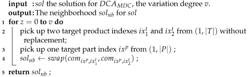
In line 3, a local search algorithm is implemented in $nbFinder(sol,v)$, and the algorithm of $nbFinder(sol,v)$ is shown in Algorithm 2. Randomly changing the components of the same part from two products to generate a new neighborhood is the major idea of $nbFinder(sol,v)$. Therefore, in line 2 and 3, the indexes of two products and the target part are selected, and the corresponding components are exchanged in the neighborhood $so{l}_{nb}$. The variation degree v is the input parameter. Larger setting of v indicates more components are swapped in $nbFinder(sol,v)$, and it means that $so{l}_{nb}$ is much different from $sol$.

Algorithm 2: The local search algorithm of $nbFinder(sol,v)$.

After generating the neighborhood, we have $sol$ and $so{l}_{nb}$, and the mission in each iteration is to determine the solution that will survive in the next iteration. The survival solution is determined in the area from line 4 to line 7. We use the label $\Delta E=q\left(sol\right)-q\left(so{l}_{nb}\right)$ to represent the gap of the solution quality between $sol$ and $so{l}_{nb}$, where $q\left(sol\right)$ returns the solution quality of $sol$, and the details of $q\left(sol\right)$ will be described in Section 4.3. The quality of $sol$ is better than $so{l}_{nb}$ when $\Delta E>0$, and $sol$ will survive in the next iteration, as shown in Line 5. Otherwise, we use the function $diverse\left(so{l}_{nb}\right)$ to determine the survival of $so{l}_{nb}$. The function $diverse\left(so{l}_{nb}\right)$ considers the acceptance threshold as shown in Equation (6), to accept $so{l}_{nb}$ or not.

$$th=exp(-\Delta E/T)$$

(6)

If $th$ is larger than the random number from $(0,1)$, $so{l}_{nb}$ is accepted, and rejected otherwise. The $so{l}_{nb}$ with worse quality is accepted in the early stage, and the probability of accepting $so{l}_{nb}$ becomes smaller as decreasing the temperatures. Therefore, we can use $diverse\left(so{l}_{nb}\right)$ to increase the solution diversity to discover more candidate solutions.

4.2. Solution Format

Assembling $\left|T\right|\times \left|P\right|$ components to $\left|T\right|$ products is the goal of $DC{A}_{MDC}$, and there are $\left|C\right|$ dimensional chains in each product. We use two data structure to represent the information of a solution, and they are the installation guidance and the sizes of all dimensional chains as illustrated in Figure 2 and Figure 5. According to Equation (2), we use a $\left|T\right|$ by $\left|P\right|$ two-dimensional array, that is named by guidance element set $GE=\left\{g{e}_{rs}\right\}$, where $1\le r\le \left|T\right|$ and $1\le s\le \left|P\right|$, to represent the installation guidance, as shown in Figure 2. Each row in $GE$ represents the components of a product, and each element $g{e}_{rs}$ saves the component index for part s. So, the assembler picks up the specific components of the installation guidance to assemble the product. The second data structure is the chain size, and a $\left|T\right|$ by $\left|C\right|$ two-dimensional array, that is named by chain size element set $CSE=\left\{cs{e}_{vw}\right\}$, where $1\le v\le \left|T\right|$ and $1\le w\le \left|C\right|$, is apply to save the chain size information. We pick up some components of a row from $GE$, calculate all chain sizes by using Equation (2), and save the chain sizes to the corresponding row in $CSE$.

4.3. Solution Quality

The solution is feasible only if the installation guidance is satisfied with the constraints of inseparability and the acceptability, as defined in Section 3.2. We use ${\Delta }_k^i$ for each product i to evaluate the product quality. The ideal product takes place when the value of ${\Delta }_k^i$ is minimized, e.g., $p{s}_k^i=c{v}_k$, and minimizing ${\Delta }_k^i$ is the goal otherwise. However, there are two dimensional chains in the bearing assembly problem, so that we have two values to evaluate the quality of the given feasible solution. The arithmetic mean is the straightforward approach of normalizing several values to one. Unfortunately, the ranges between $l{b}_k$ and $u{b}_k$ of all dimensional chains may be different. For example, the range of chain number one is $0.05+0.2=0.25$ and $0.15+0.18=0.33$ for chain number two in Table 2. Considering that the ($p{s}_1^i$, $p{s}_2^i$) are (0.39, 0.25) and (0.2, 0.43) for the bearing i and $i+1$, the values of ${\Delta }_k^i$ are (0.19, 0) and (0, 0.18), respectively, and the arithmetic mean values are 0.095 and 0.09. For the perspective of the arithmetic mean, the product $i+1$ is better than the product i because of $0.095>0.09$. However, ${\Delta }_1^i$ does not meet $u{b}_1$, but ${\Delta }_2^{i+1}$ meets $u{b}_2$, so product i is better than the product $i+1$ for the perspective of minimizing ${\Delta }_k^i$. We have no ideas of ways to distinguish which one is better by the arithmetic mean. Thus, the arithmetic mean is inappropriate in measuring the solution quality in $DC{A}_{MDC}$.

To determine the solution quality, we have to consider following two issues in the $DC{A}_{MDC}$ problem:

• Asymmetry tolerance $a{t}_k^i$: the $l{b}_k$ and $u{b}_k$ may be different.
• Multiple dimensional chains: each product i has some ${\Delta }_k^i$.

We have to normalize the above scores to one value to represent the solution quality of the give product. The asymmetry tolerance $a{t}_k^i$ is defined in Equation (7). Each ${\Delta }_k^i$ is normalized by the tolerance range, i.e., $l{b}_k$ or $u{b}_k$, so the tolerance could be estimated in the same criteria.

$$a{t}_k^i=\left\{\begin{array}{ccc}\hfill (p{s}_k^i-c{v}_k)/l{b}_k& & if p{s}_k^i<c{v}_k,\hfill \\ \hfill (p{s}_k^i-c{v}_k)/u{b}_k& & otherwise.\hfill \end{array}\right.$$

(7)

The relationship between the product size $p{s}_k^i$, $c{v}_k$, $l{b}_k$, and $u{p}_k$ is illustrated in Figure 6. We use three products to explain the calculation of the solution quality, where $p{s}_k^1=0.06$, $p{s}_k^2=0.2$, and $p{s}_k^3=0.39$. The product 2 is optimal because of ${\Delta }_k^2=0$. The quality of product 1 is $a{t}_k^1=(0.06-0.2)/-0.15=-0.14/-0.15=0.93$ for k-th part, and the quality of product 3 for the part k is $a{t}_k^3=(0.39-0.2)/0.2=0.19/0.2=0.95$. The distance from $p{s}_k^1$ to $c{v}_k+l{b}_k$ and $p{s}_k^3$ to $c{v}_k+u{b}_k$ is the same, but $a{t}_k^3>a{t}_k^1$ because of $u{b}_k>l{b}_k$. So, $a{t}_k^i$ can correctly describe the solution quality. Moreover, the product is feasible only when $a{t}_k\le 1$ for k-th part and infeasible otherwise.

The other consideration of multiple dimensional chains indicates that each product has $\left|P\right|$ values of $a{t}_k^i$. We consider the maximum $a{t}_k^i$ to represent the quality of the product i as defined in Equation (8). The worst $a{t}_k^i$ could be treated as the quality bottleneck, and the product quality is improved when the worst $a{t}_k^i$ is decreased. Therefore, applying Equation (8) to be the solution quality is reasonable.

$$q_i=\underset{\forall k}{max}a{t}_k^i$$

(8)

Thus, the solution quality $q\left(sol\right)$ is derived as shown in Equation (9) by the same concept of Equation (8).

$$q\left(sol\right)=\underset{\forall i}{max}{q}_i$$

(9)

4.4. Tracing $AG{O}_{MDC}$

In this section, the example listed in Table 1 is applied to trace the proposed $AG{O}_{MDC}$ in finding the solution of $DC{A}_{MDC}$. The major mission is to demonstrate the processes of $AG{O}_{MDC}$ in solving the problem. Therefore, the solutions and the algorithm status in each iteration are saved, and the solution might not be optimized.

In the beginning, $AG{O}_{MDC}$ receives the composition diagram illustrated in Figure 1, the size information shown in Figure 4, and the product specification listed in Table 2, and the algorithm configuration. Initial temperature 50, temperature descent rate 0.98, and the maximum round 10 are considered. To focus on introducing the process of $AG{O}_{MDC}$, the entire information of solutions and algorithm status is listed in Appendix A.

From

Table A1. The solution details in each iteration derived by $AG{O}_{MDC}$ for the example listed in Table 1.

Iteration	i	${wp}_{jx}$	${ps}_1^i$	${ps}_2^i$	${at}_1^i$	${at}_2^i$	$q_i$	$q\left(sol\right)$
1	1	(3, 2, 3)	0.2	0.28	0	0.17	0.17	1.8
	2	(0, 0, 0)	0.11	0.17	0.18	0.53	1.8
	3	(1, 3, 1)	0.3	0.3	0.5	0.28	0.5
	4	(2, 1, 2)	0.28	0.33	0.4	0.44	0.44
2	1	(3, 2, 2)	0.2	0.31	0	0.33	0.33	1.8
	2	(0, 0, 0)	0.11	0.17	0.18	0.53	1.8
	3	(1, 3, 1)	0.3	0.3	0.5	0.28	0.5
	4	(2, 1, 3)	0.28	0.3	0.4	0.28	0.4
3	1	(3, 2, 0)	0.2	0.18	0	0.47	0.47	1.8
	2	(0, 0, 2)	0.11	0.3	0.18	0.28	1.8
	3	(1, 3, 1)	0.3	0.3	0.5	0.28	0.5
	4	(2, 1, 3)	0.28	0.3	0.4	0.28	0.4
4	1	(3, 2, 0)	0.2	0.18	0	0.47	0.47	0.6
	2	(2, 0, 2)	0.17	0.3	0.6	0.28	0.6
	3	(1, 3, 1)	0.3	0.3	0.5	0.28	0.5
	4	(0, 1, 3)	0.22	0.3	0.4	0.28	0.28
5	1	(3, 2, 0)	0.2	0.18	0	0.47	0.47	0.5
	2	(1, 0, 2)	0.23	0.3	0.6	0.28	0.28
	3	(2, 3, 1)	0.24	0.3	0.5	0.28	0.28
	4	(0, 1, 3)	0.22	0.3	0.1	0.28	0.28
6	1	(3, 2, 0)	0.2	0.18	0	0.47	0.47	0.5
	2	(1, 0, 2)	0.23	0.3	0.15	0.28	0.28
	3	(0, 3, 1)	0.18	0.3	0.4	0.28	0.4
	4	(2, 1, 3)	0.28	0.3	0.4	0.28	0.4
7	1	(3, 2, 0)	0.2	0.18	0	0.47	0.47	0.5
	2	(1, 0, 2)	0.23	0.3	0.15	0.28	0.28
	3	(2, 3, 1)	0.24	0.3	0.2	0.28	0.28
	4	(0, 1, 3)	0.22	0.3	0.1	0.28	0.28
8	1	(3, 2, 0)	0.2	0.18	0	0.47	0.47	0.5
	2	(1, 0, 2)	0.23	0.3	0.15	0.28	0.28
	3	(2, 3, 1)	0.24	0.3	0.2	0.28	0.28
	4	(0, 1, 3)	0.22	0.3	0.1	0.28	0.28
9	1	(0, 2, 0)	0.18	0.18	0.4	0.47	0.47	1
	2	(1, 0, 2)	0.23	0.3	0.15	0.28	0.28
	3	(2, 3, 1)	0.24	0.3	0.2	0.28	0.28
	4	(3, 1, 3)	0.15	0.3	0.1	0.28	1
10	1	(1, 2, 0)	0.3	0.18	0.5	0.47	0.5	1.8
	2	(0, 0, 2)	0.11	0.3	1.8	0.28	1.8
	3	(2, 3, 1)	0.24	0.3	0.2	0.28	0.28
	4	(3, 1, 3)	0.15	0.3	1	0.28	1

, the initial solution does not fit the acceptability because $q\left(sol\right)=1.8$. In the first ten iterations, the neighbors with higher quality are accepted in iteration three, four, and nine, and the solutions with lower quality are accepted in iteration number eight. In other iterations, the neighbors with the same quality are accepted, since the random value is larger than the value of $th$ that is defined in Equation (6). The details in terms of solutions and algorithm status are listed in Table A1 and

Table A2. The algorithm status in each iteration for the example listed in Table 1.

Iteration	T	$q\left(sol\right)$	$q\left({sol}_{nb}\right)$	$\Delta E$	th	Random Value	Accept $q\left({sol}_{nb}\right)$
1	100	1.8	1.8	0	1	0.74	Yes
2	98	1.8	1.8	0	1	0.18	Yes
3	96.04	1.8	0.6	1.2	N/A	N/A	Yes
4	94.12	0.6	0.5	0.1	N/A	N/A	Yes
5	92.24	0.5	0.5	0	1	0.4	Yes
6	90.39	0.5	0.5	0	1	0.52	Yes
7	88.58	0.5	0.5	0	1	1	No
8	86.81	0.5	1	−0.5	1.01	0.59	Yes
9	85.08	1	1.8	−0.8	1.01	0.69	Yes
10	83.37	1.8	1.8	0	0.99	0.9	Yes

, respectively. However, in iteration seven, the neighbor has the same quality with that of the current solution, but the neighbor is rejected. The value of $th$ is one which means that accepting the neighbor in high probability, but the random value is one. Therefore, the neighbor is rejected, and the current solution survives in the next iteration.

The results show the process of the proposed $AG{O}_{PDC}$, and the information in terms of accepting neighbors is displayed in Table A2. In the early stage, $AG{O}_{MDC}$ accepts the neighbors with lower quality in high probability. As decreasing the temperatures, the value of $th$ becomes lower and lower. The solution quality would be improved by considering more iterations.

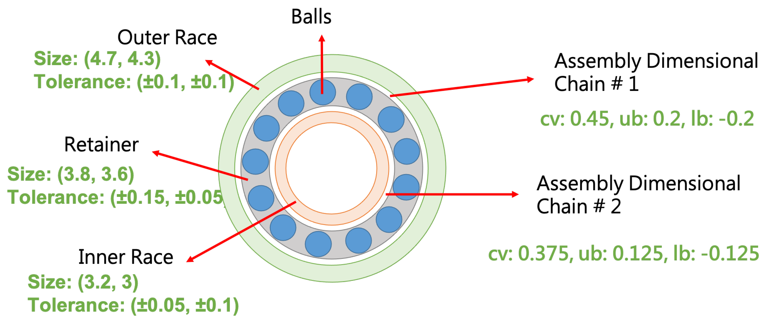
5. Simulation

The real-world bearing assembly process is considered, and the CAD size and the assembly specification are illustrated in Figure 7, and they are calculated by the dimensional chain analysis during the product design phase. The real-world size data of $43\times 3$ components, i.e., 43 bearings will be produced, are collected and the simulation instance generator is developed based on the collected size data. The simulated size data generated by the simulation instance generator is helpful in increasing the diversity of the simulation. The specification of the simulation platform is CPU i7-7700, RAM 16 GB, SSD 128 G, and using Visual Studio C++ to implement $AG{O}_{MDC}$. In the following simulations, we focus on analyzing the solution quality generated by the proposed $AG{O}_{MDC}$ and provide the optimized algorithm configuration for the manager of the assembly line in the company.

5.1. Feasibility Analysis

The algorithm configuration ($T,r,iter$) = (5000, $0.98$, $10,000$) is considered in this simulation to evaluate the effectiveness in resolving $DC{A}_{MDC}$. The setting is identical to the suggestion proposed in [17]. Moreover, $v=1$ is applied to $AG{O}_{MDC}$ to carefully trace the variance of neighborhood solutions. Each instance runs ten times, and the values are averaged for the final score. $AG{O}_{MDC}$ consumes 562.6 ms to derive the solution with quality 0.51384 on average. The variation of the solution quality is illustrated in Figure 8. The processes of $AG{O}_{MDC}$ include three phases: the exploration stage in the first 1000 iterations, the convergence stage from iteration 1000 to 4800, and the stable stage after iteration 4800. In the exploration stage, $AG{O}_{MDC}$ tries its best to reach all kinds of solutions that also include the solutions with worse quality. In the convergence stage, the solution quality is improved slowly by accepting better solutions in high probability. Accepting a lower quality solution is possible, but the possibility is not high. Eventually, the solution quality is not improved, obviously because the temperature is low. The possibility of accepting the worse solution is based on the temperature and the quality of the neighborhood solution. Higher temperatures and higher solution quality result in higher possibility of accepting neighborhood solutions. The curve illustrated in Figure 8 demonstrates the relationship between the probability of accepting lower quality solution and the algorithm configurations. Therefore, the proposed $AG{O}_{MDC}$ resolves $DC{A}_{MDC}$ and the running time is rational for the implementation consideration.

In the first 1000 iterations, the solution quality dramatically changes and becomes stable in the following iterations. The final solution quality is 0.51384 on average. The $nbFinder\left(sol\right)$ in $AG{O}_{MDC}$ exchanges the components of two products for the same part. $AG{O}_{MDC}$ follows Equation (2) to calculate the solution quality, so the inseparability is realized. The final solution quality is 0.51384 that is smaller than 1, so the acceptability is matched. Eventually, the solution derived by $AG{O}_{MDC}$ is feasible.

Moreover, the solution quality is larger than 1 during the first 1000 iterations, and it implies that the solution derived by $AG{O}_{MDC}$ is infeasible. In the early stage, the value of T is hight, so the value of $th$ is closed to 1 according to Equation (6). So, $AG{O}_{MDC}$ accepts the neighbors with worse solution quality in high probability. When T is decreased, the probability of accepting the solutions with worse quality is also decreased. In the early stage, $AG{O}_{MDC}$ seeks the solutions widely, and the search strategy changes to seek the elite solution after some iterations. If $AG{O}_{MDC}$ only accepts better solutions, the initial solution determines the quality of the output solution. Therefore, the solution quality that the algorithm only accepts elite solutions may be worse than the acceptance strategy applied in $AG{O}_{MDC}$.

5.2. Configuration Optimization

In this simulation, we use the cases that we received from the company to design the simulation case generator. The product specification as shown in Figure 7 is the input of the case generator, and then the case generator outputs the component sizes. So, we can evaluate the performance of $AG{O}_{MDC}$ by variant problem instances to study the optimized configuration. We investigate two issues that are the number of products and the product precision and provide the algorithm configuration for the manager of the assembly line. We consider the following three steps to find out the suggested configuration: (1) find out the optimal setting of the temperature descent rate r by considering the adequate settings; (2) using the derived r to analyze the setting of the maximum iteration; (3) calculating the initial temperature T, and the details are as shown below.

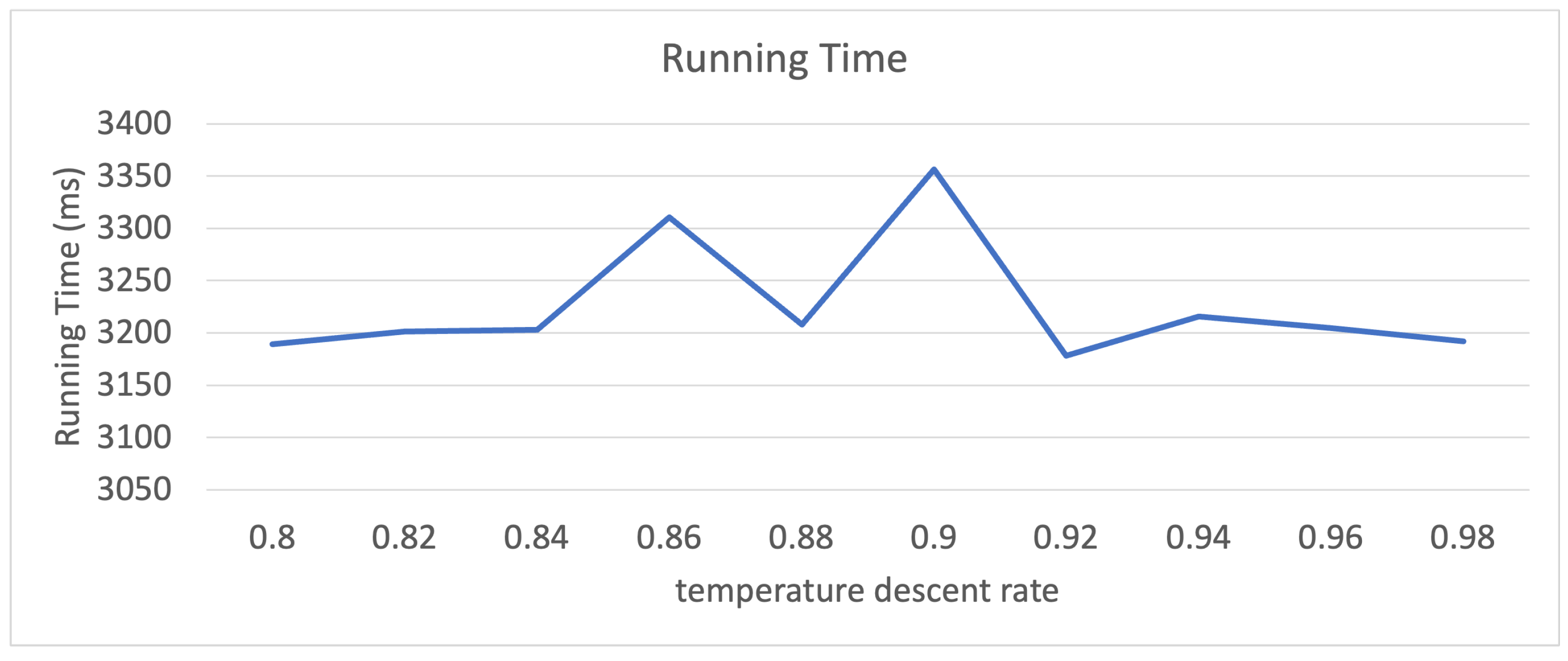
• The setting of the temperature descent rate r. To calculate the optimal setting of r, we evaluate the performance of various settings of v with the other extreme settings, and they are $T=5000$, $iter=10,000$, and the number of products is 250. The results of the solution quality and the running time are illustrated in Figure 9 and Figure 10, respectively. The setting of $r=0.9$ provides higher solution quality than that of others, while the corresponding running time is 3350 (ms). The time required by $AG{O}_{MDC}$ to calculate the solution is acceptable. Therefore, we consider $r=0.9$ in the following simulations.

Figure 9. The solution quality variation for different temperature descent rate.

Figure 9. The solution quality variation for different temperature descent rate.

Figure 10. The running time variation for different temperature descent rate.

Figure 10. The running time variation for different temperature descent rate.

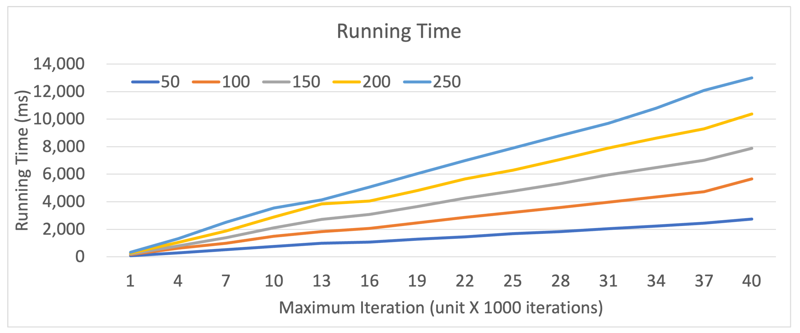
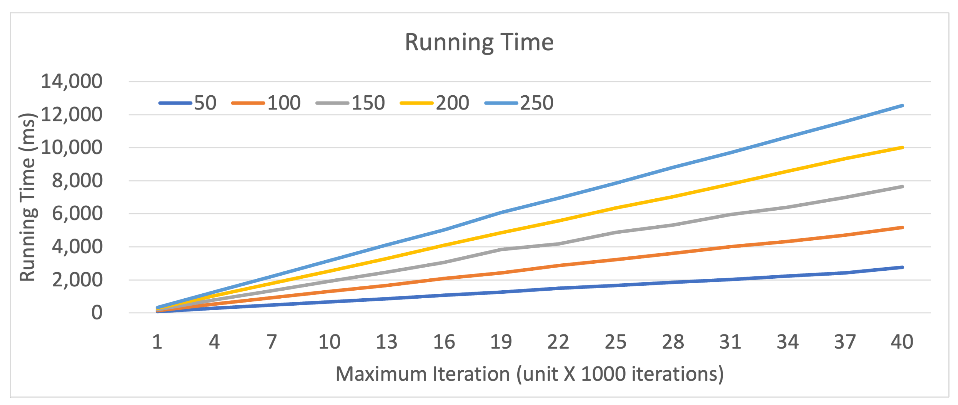
• The setting of the maximum iteration. Considering $r=0.9$ is derived from the above simulations, we evaluate the performance of the proposed $AG{O}_{MDC}$ under the settings of maximum iterations from 500 to 5000 with the gap 500. The simulation results of the solution quality and the running time are illustrated in Figure 11 and Figure 12, respectively. The solutions in 50 and 100 products are acceptable after 1000 rounds, and the case with 150 products requires 3000 rounds. However, we should provide more iterations to calculate acceptable solutions in the cases with 200 and 250 products. The running time illustrated in Figure 12 is still acceptable in all instances, so we design the simulation with longer algorithm execution time to calculate the feasible solutions.

Figure 11. The solution quality variation captured from the instances with different maximum iterations and $r=0.9$ in different problem scales.

Figure 11. The solution quality variation captured from the instances with different maximum iterations and $r=0.9$ in different problem scales.

Figure 12. The running time variation captured from the instances with different maximum iterations and $r=0.9$ in different problem scales.

Figure 12. The running time variation captured from the instances with different maximum iterations and $r=0.9$ in different problem scales.

It is difficult to find out the relationship between the problem scale and the minimum iterations for reaching the feasible solutions when two variables are considered: the initial temperature and the maximum iteration. Thus, we consider three levels of the initial temperatures: low level $T=300$, medium level $T=1300$, and high level $T=2300$ to evaluate performance under various settings of the maximum iteration. Moreover, minimizing $a{t}_k^i$ is the objective in $DC{A}_{MDC}$, but the products with the quality $a{t}_k^i\le 1$ are feasible. From the perspective of the implementation, $a{t}_k^i=0$ is optimal, but $q\left(sol\right)=0.8$ is acceptable. The products with $a{t}_k^i=0.9$ are also feasible, but if the products will be assembled with other parts, 20% tolerance is more appropriate than that of 10%. Therefore, the goal of this simulation is to capture the performance of various maximum iterations under three levels of the initial temperatures when the solution quality converges to $q\left(sol\right)\le 0.8$.

The simulation results are illustrated in Figure 13 for the solution quality and Figure A1–Figure A3 for the running time. We observed that three curves are overlapping in each sub-graph. The curve variance is slight in different levels of the initial temperatures, so various initial temperatures do not affect the convergence too much. Moreover, the solution quality meets the objective $q\left(sol\right)\le 0.8$ in all instances eventually. We list the thresholds of the initial temperatures when reaching $q\left(sol\right)\le 0.8$, and the results are shown in

Table 3. The settings of maximum iterations that result in the solution quality $q\left(sol\right)\le 0.8$. The maximum threshold in each problem scale is marked in bold style.

	Low Level	Medium Level	High Level
50	4000	4000	4000
100	4000	4000	4000
150	13,000	10,000	13,000
200	22,000	22,000	19,000
250	31,000	34,000	34,000

. The maximum threshold in each problem scale is marked in bold style. The increment of the temperature threshold is proportional to the problem scale linearly for the problems with more than 100 products, so we can use the linear regression analysis to find out the increment function. The instances with 50 products and 100 products require the same maximum iterations, so we consider the number of products from 100 to 250. Using the data in Table 3, we apply the linear regression analysis [45,46] to derive the recommended maximum iteration, as shown in Equation (9), where z is the number of products. Therefore, we can use Equation (10) to recommend the appropriate settings of the maximum iteration $f\left(z\right)$ ot derive expected solution quality 0.8.

$$f\left(z\right)=200z-16,000$$

(10)

• The setting of the initial temperature. We consider $r=0.9$ and the maximum iterations determined by Equation (10) to find out the optimal settings of initial temperatures from 1000 to 40,000 with gap 3000. The results are illustrated in Figure 14. Since the running time is acceptable that is evaluated in the above simulations, we skip the discussion of the running time. From Figure 14, we have the following observations: (1) all results are bounded by $q\left(sol\right)=0.8$; (2) various initial temperatures do not affect the solution quality too much; (3) the curves of solution quality are bounded within 0.7 and 0.8. The solution result means that the initial temperatures slightly affect the solution quality, but not too much. Therefore, the initial temperatures could be selected from 1000 to 40,000 arbitrarily, and the solution quality would be better than 0.8.

5.3. Discussion

According to the results from the above simulations, the recommended configuration of deriving the solution quality better than 0.8 is listed as follows:

• The initial temperature: the values should be larger than 1000.
• The temperature descent rate: $0.9$ provides high probability in reaching the solutions with higher quality than others.
• The maximum iteration: using Equation (10) to determines the maximum iteration $f\left(z\right)$ for the number of products z.

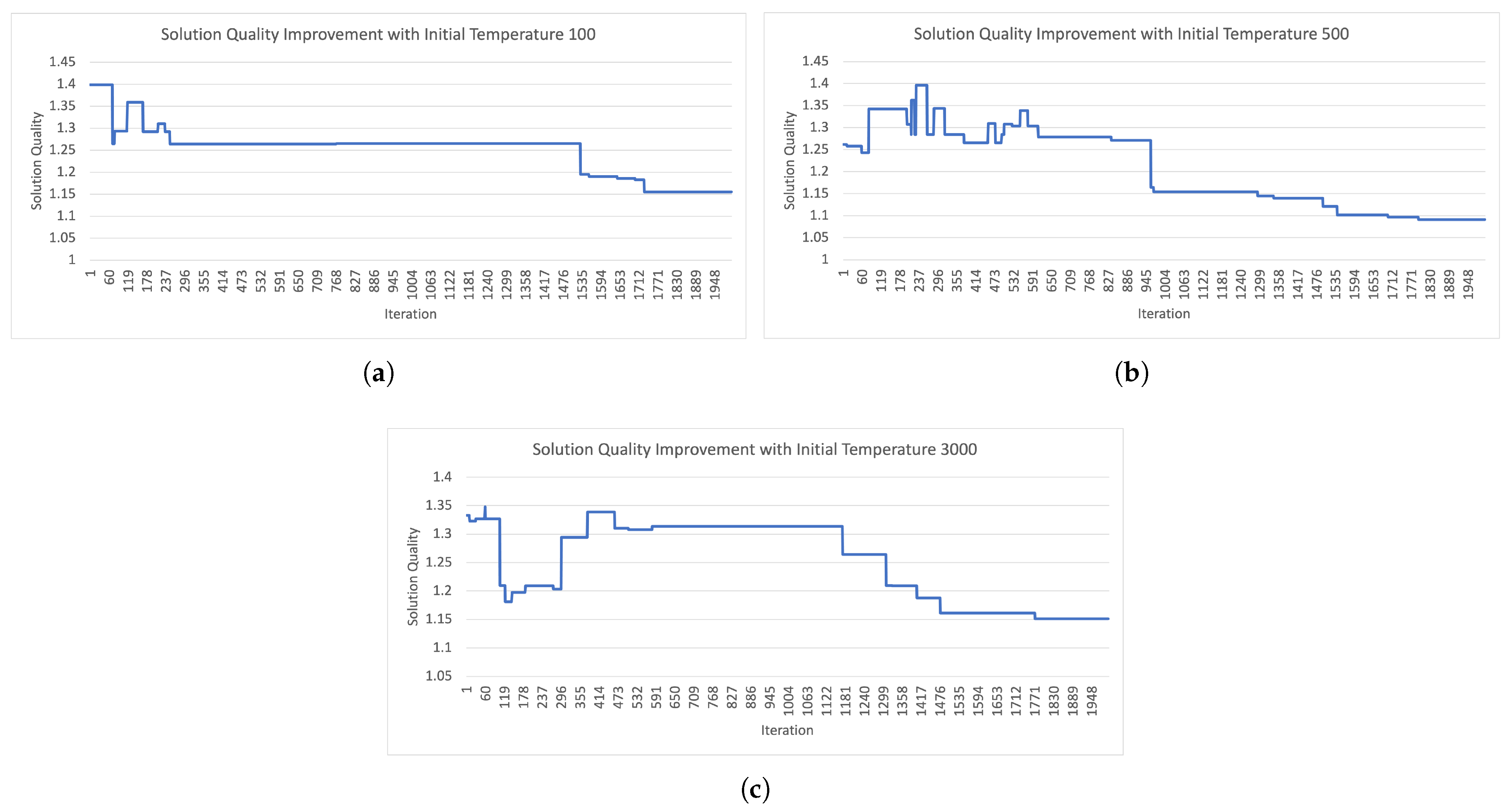
We did not find the specific setting of initial temperature in the above simulations. The initial temperatures determine the decision on accepting the solutions with lower quality. According to the acceptance threshold defined in Equation (6), the probability of accepting the worse quality solution in higher temperatures is larger than that in lower temperatures. Thus, the initial temperatures determine the search breadth, and that also affects the solution quality indirectly. We organize the simulations to confirm the assumption. We consider $r=0.9$ to observe the solution quality variation in the first 2000 iterations for assembling 150 products. The results captured from the initial temperatures 100, 500, and 3000 are illustrated in Figure 15. The degree of the curve variation becomes larger as the initial temperatures are increased, and the solutions with different properties can be reached with high probability. Moreover, higher temperatures not only increase the acceptance probability, but also determine the accepted solution quality. In Figure 15c, the curve suddenly raised in round 300, and the amount is larger than that in Figure 15a,b. So higher temperatures would help on effectively probing various properties of solutions than the lower settings.

Wider search results in higher probability of reaching the solutions with better quality theoretically. Therefore, the manager could increase the setting of the initial temperatures to improve the probability in reaching better solutions if the solution does not reach the expected goal.

6. Conclusions

Most products or modules are assembled by several parts, and the bearing discussed in this article consists of three parts and two surfaces. The major difficulty is that some dimensional chains would cross on the same part, so the gaps between different dimensional chains that crossed on the same part should be evaluated without separation. The proposed $AG{O}_{MDC}$ considers the inseparability to compute the assembly guidance for assemblers. From the simulation results, the solutions derived by $AG{O}_{MDC}$ are satisfied with the constraints of inseparability and acceptability. For the implementation, the appropriate algorithm configurations are suggested to find the solutions with acceptable product quality. Moreover, the running time of calculating the solution is not higher than 2 s for 250 products. Thus, the running time is low enough to be applied to move the modules from manufacturing lines to assembly lines. Therefore, the proposed approach provides high possibility of implementation.

Optimizing the algorithm configurations is the major objective of solving the optimization problems. However, the optimal solution is not the first concern in manufacturing because the real-world processes would consider more additional issues, e.g., labor cost and the rework time. Since the manufacturing cost comes from several issues, minimizing the cost without decreasing the product quality is the major concern of most companies. The producing managers prefer to find out the balance between the solution quality and the manufacturing cost rather than reaching the quality optimality. On the other hand, the scheduling becomes more important as the automated manufacturing is getting popular. Once the assembly guidance is prepared, the assembly lines could automatically assemble the products according to the assembly guidance. Therefore, the proposed $AG{O}_{MDC}$ provides critical contributions on the integration about automated manufacturing.