
On the Solutions of the b-Family of Novikov Equation

Abstract
:1. Introduction
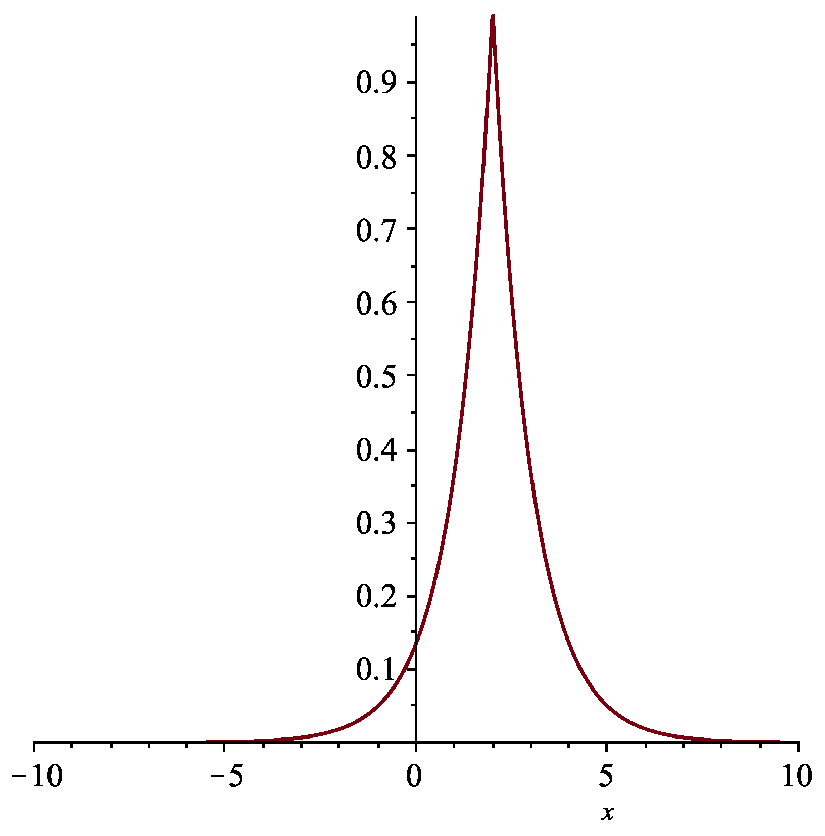
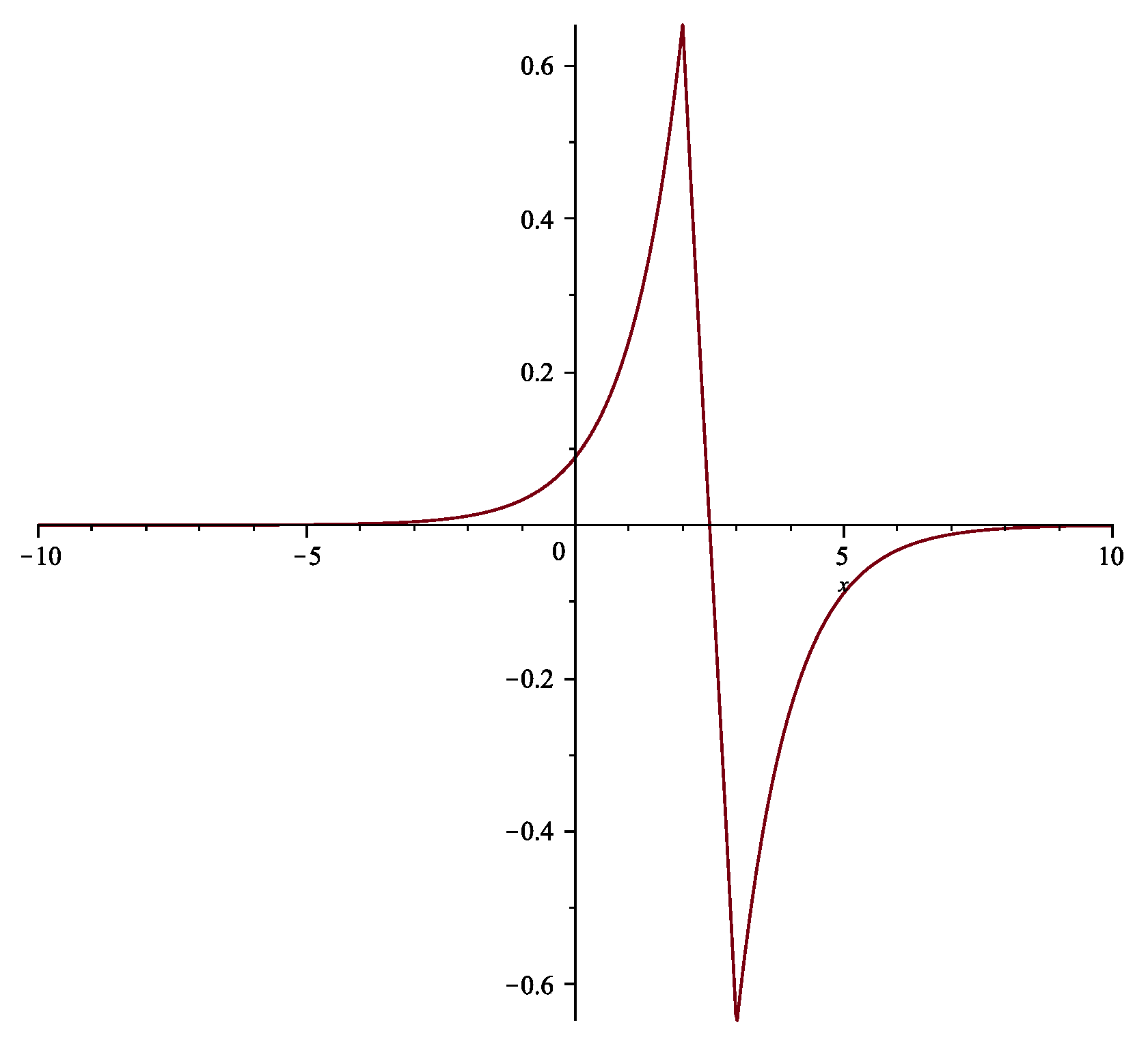
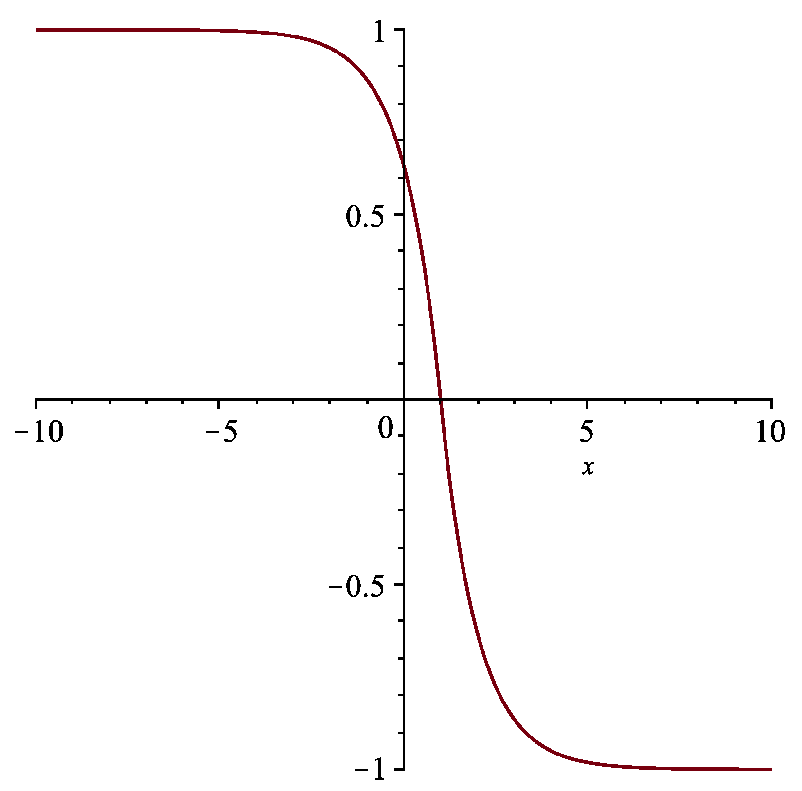
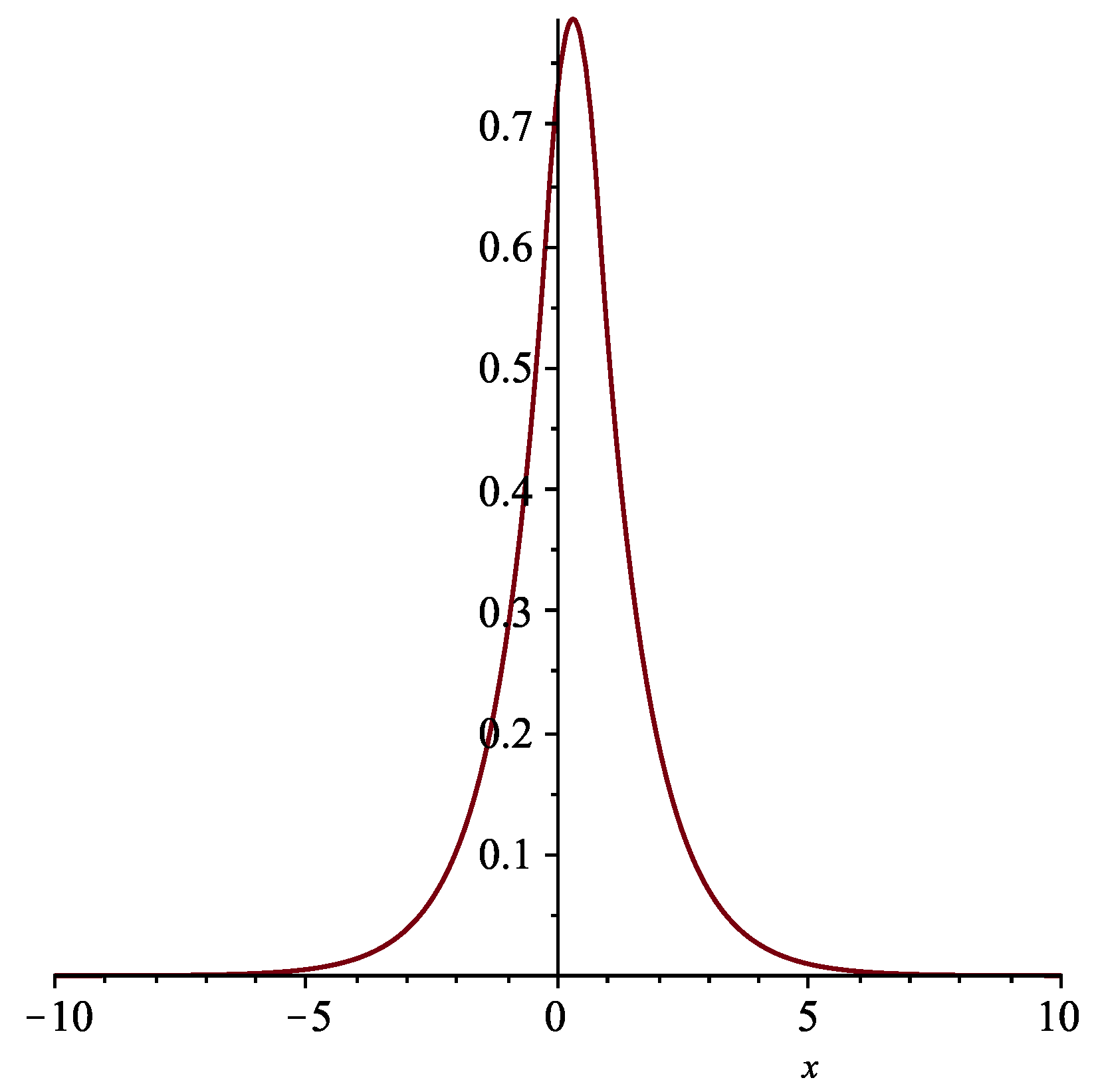
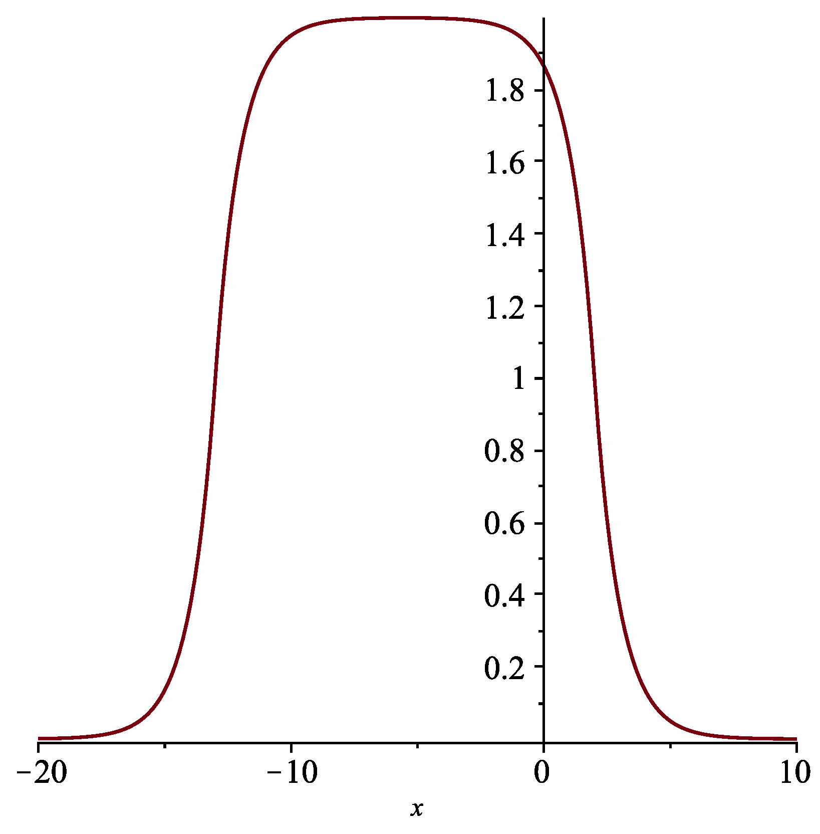
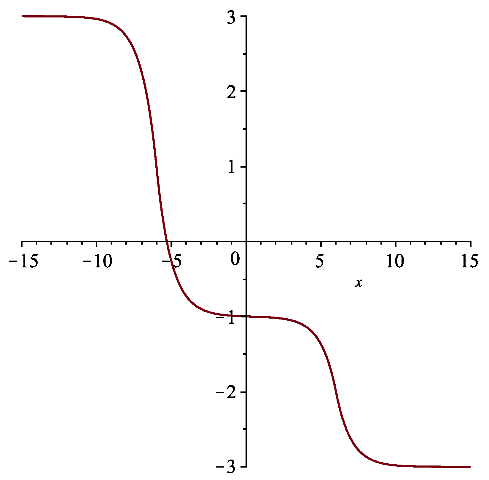
2. Peakon Solutions
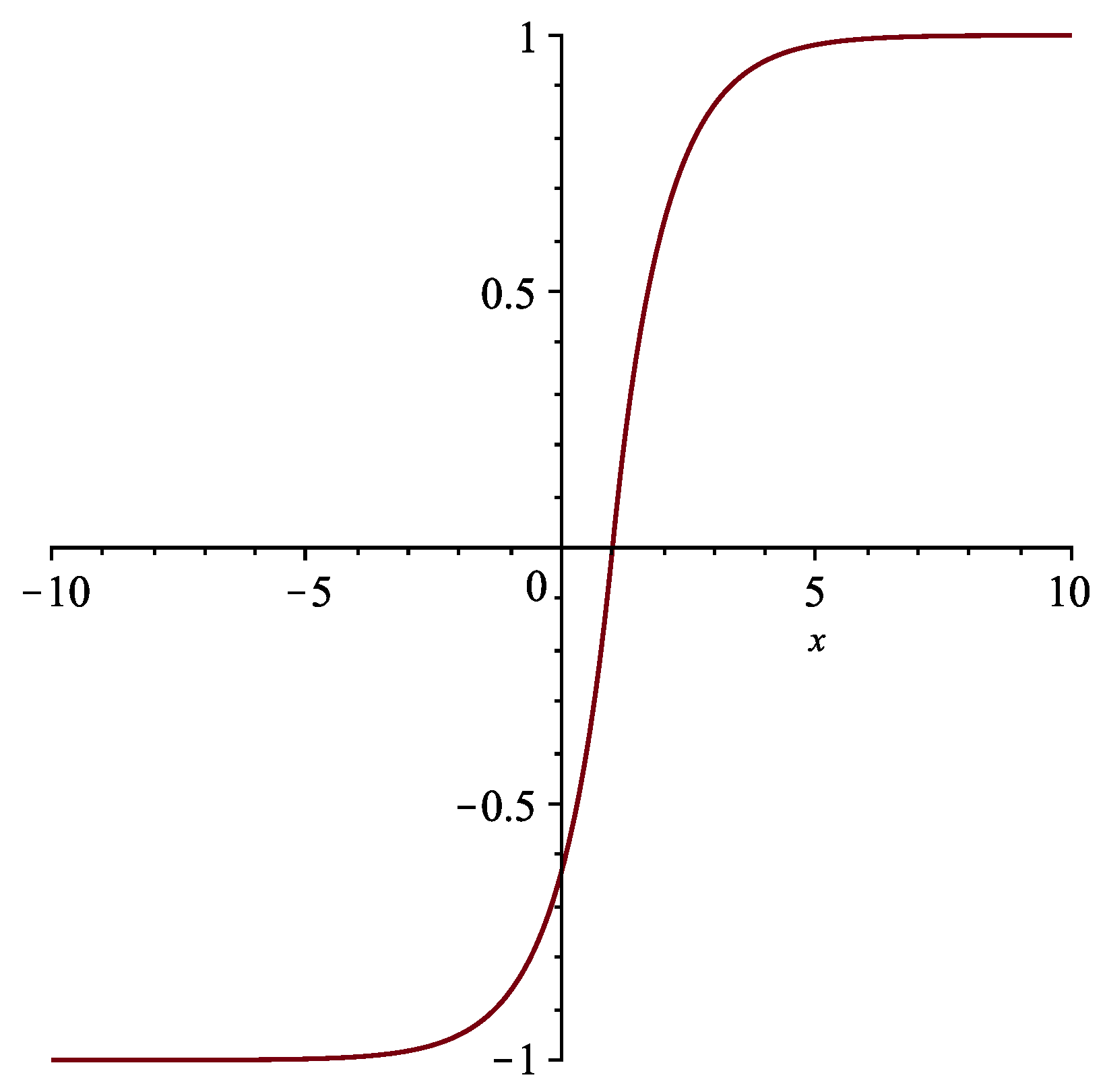
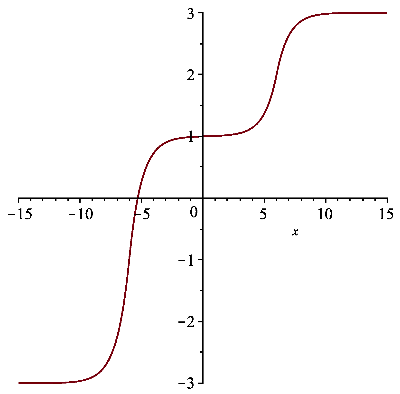
3. Kink and Smooth Soliton Solutions
Author Contributions
Funding
Institutional Review Board Statement
Informed Consent Statement
Data Availability Statement
Acknowledgments
Conflicts of Interest
References
- Holm, D.; Staley, M. Nonlinear balance and exchange of stability of dynamics of solitons, peakons, ramps/cliffs and leftons in a 1 + 1 nonlinear evolutionary PDE. Phys. Lett. A 2003, 308, 437–444. [Google Scholar] [CrossRef] [Green Version]
- Holm, D.; Staley, M. Wave structure and nonlinear balance in a family of 1 + 1 evolutionary PDE’s. SIAM J. Appl. Dyn. Syst. 2003, 2, 323–380. [Google Scholar] [CrossRef] [Green Version]
- Xia, B.; Qiao, Z. The N-kink, bell-shape and hat-shape solitary solutions of b-family equation in the case of b = 0. Phys. Lett. A 2013, 377, 2340–2342. [Google Scholar] [CrossRef]
- Fokas, A.; Fuchssteiner, B. Symplectic structures, their Bäklund transformation and hereditary symmetries. Physica D 1981, 4, 47–66. [Google Scholar]
- Camassa, R.; Holm, D. An integrable shallow water equation with peaked solitons. Phys. Rev. Lett. 1993, 71, 1661–1664. [Google Scholar] [CrossRef] [PubMed] [Green Version]
- Fisher, M.; Fisher, J. The Camassa-Holm equation: Conserved quantities and the initial value problem. Phys. Lett. A 1999, 259, 371–376. [Google Scholar] [CrossRef] [Green Version]
- Constantin, A. The trajectories of particles in Stokes waves. Invent. Math. 2006, 166, 523–535. [Google Scholar] [CrossRef]
- Constantin, A.; Escher, J. Particle trajectories in solitary water waves. Bull. Am. Math. Soc. 2007, 44, 423–431. [Google Scholar] [CrossRef] [Green Version]
- Constantin, A.; Escher, J. Analyticity of periodic traveling free surface water waves with vorticity. Ann. Math. 2011, 173, 559–568. [Google Scholar] [CrossRef] [Green Version]
- Degasperis, A.; Procesi, M. Asymptotic Integrability. In Symmetry and Perturbation Theory; World Scientific Publishing: River Edge, NJ, USA; Rome, Italy, 1998; pp. 23–37. [Google Scholar]
- Constantin, A.; Lannes, D. The hydrodynamical relevant of the Camassa-Holm and Degasperis-Procesi equations. Arch. Ration. Mech. Anal. 2009, 192, 165–186. [Google Scholar] [CrossRef] [Green Version]
- Degasperis, A.; Holm, D.; Hone, A. A new Integrable equation with peakon solutions. Theor. Math. Phys. 2002, 133, 1463–1474. [Google Scholar] [CrossRef] [Green Version]
- Mi, Y.; Mu, C. On the Cauchy problem for the modified Novikov equation with peakon solutions. J. Differ. Equ. 2013, 254, 961–982. [Google Scholar] [CrossRef]
- Novikov, V. Generalizations of the Camassa-Holm equation. J. Phys. A Math. Theor. 2009, 42, 342002. [Google Scholar] [CrossRef]
- Hone, W.; Wang, J. Integrable peakon equations with cubic nonlinearity. J. Phys. A Math. Theor. 2008, 41, 372002. [Google Scholar] [CrossRef]
- Hone, W.; Lundmark, H.; Szmigielski, J. Explicit multipeakon solutions of Novikov cubically nonlinear integrable Camassa-Holm type equation. Dyn. Partial Differ. Equ. 2009, 6, 253–289. [Google Scholar] [CrossRef]


Publisher’s Note: MDPI stays neutral with regard to jurisdictional claims in published maps and institutional affiliations. |
© 2021 by the authors. Licensee MDPI, Basel, Switzerland. This article is an open access article distributed under the terms and conditions of the Creative Commons Attribution (CC BY) license (https://creativecommons.org/licenses/by/4.0/).
Share and Cite
Wang, T.; Han, X.; Lu, Y. On the Solutions of the b-Family of Novikov Equation. Symmetry 2021, 13, 1765. https://doi.org/10.3390/sym13101765
Wang T, Han X, Lu Y. On the Solutions of the b-Family of Novikov Equation. Symmetry. 2021; 13(10):1765. https://doi.org/10.3390/sym13101765
Chicago/Turabian StyleWang, Tingting, Xuanxuan Han, and Yibin Lu. 2021. "On the Solutions of the b-Family of Novikov Equation" Symmetry 13, no. 10: 1765. https://doi.org/10.3390/sym13101765
APA StyleWang, T., Han, X., & Lu, Y. (2021). On the Solutions of the b-Family of Novikov Equation. Symmetry, 13(10), 1765. https://doi.org/10.3390/sym13101765