Abstract
The traditional procedure of predicting the settling velocity of a spherical particle is inconvenient as it involves iterations, complex correlations, and an unpredictable degree of uncertainty. The limitations can be addressed efficiently with artificial intelligence-based machine-learning algorithms (MLAs). The limited number of isolated studies conducted to date were constricted to specific fluid rheology, a particular MLA, and insufficient data. In the current study, the generalized application of ML was comprehensively investigated for Newtonian and three varieties of non-Newtonian fluids such as Power-law, Bingham, and Herschel Bulkley. A diverse set of nine MLAs were trained and tested using a large dataset of 967 samples. The ranges of generalized particle Reynolds number (ReG) and drag coefficient (CD) for the dataset were 10−3 < ReG (-) < 104 and 10−1 < CD (-) < 105, respectively. The performances of the models were statistically evaluated using an evaluation metric of the coefficient-of-determination (R2), root-mean-square-error (RMSE), mean-squared-error (MSE), and mean-absolute-error (MAE). The support vector regression with polynomial kernel demonstrated the optimum performance with R2 = 0.92, RMSE = 0.066, MSE = 0.0044, and MAE = 0.044. Its generalization capability was validated using the ten-fold-cross-validation technique, leave-one-feature-out experiment, and leave-one-data-set-out validation. The outcome of the current investigation was a generalized approach to modeling the settling velocity.
1. Introduction
Settling velocity (Vs) is the constant free-falling velocity of a solid particle in a stationary liquid when the opposing gravity and drag forces acting on the particle approximately equals one another. It is a significant parameter in the industries that involve solid–liquid two-phase flows. Probably, the most important examples are the slurry transportation in minerals and coal processing, wastewater treatment, dredging, hydraulic fracturing, and drilling operations. It is also essential to the fluidized bed as applied for catalysis, adsorption, ion exchange, water softening, and food processing. The concept of Vs is also vital in mixing operations. In these applications, the settling velocities of amorphous particles experiencing hindrances from the walls, adjacent particles, and the flow conditions in both Newtonian and non-Newtonian liquids are of practical interest. Interestingly, this kind of non-ideal settling velocity in complex operating conditions can be correlated to the ideal Vs of a spherical particle measured with a lab-scale setup or predicted using a reliable model. That is why both measuring and predicting Vs in all kinds of fluids are active research interests since the 1850s [1,2,3,4,5,6,7,8,9,10,11,12,13,14,15,16,17,18,19,20,21,22,23,24,25].
Correlating the settling velocity of spherical particles to the measurable properties of liquid and solid was the primary focus of the previous studies. Most of the existing correlations were developed based on the following non-dimensional groups for Newtonian fluids:
Drag coefficient:
Particle Reynolds number:
where,
- ρs: solid density (kg/m3)
- ρl: liquid density (kg/m3)
- d: particle diameter (m)
- g: gravitational acceleration (m/s2)
- μl: viscosity of Newtonian liquid (Pa.s)
The hydrodynamic complexities associated with Vs are considered to be sufficiently captured with CD and Rep. The idea of correlating CD to Rep was pioneered by Stokes with a single-parameter equation: [9]. The limitation of this model is that it is applicable only if Rep < 0.1. Based on the Stokes law, many empirical and semi-empirical correlations have been developed afterward. For example, the CD-Rep correlation proposed by Cheng was found to perform better compared to seven (7) other similar models [4]. All of these models were developed for spherical particles in Newtonian fluids. The Cheng correlation is presented with Equation (3).
Although applying this kind of correlation is comparatively easier for a Newtonian fluid, a similar application to a non-Newtonian fluid is not convenient at all. Modeling complex non-Newtonian rheology is a difficult task [2,5,7,8,12,16,19,20,21,23,24,25,26,27]. Nevertheless, a CD-Rep correlation can be used to predict Vs in a non-Newtonian fluid by replacing Rep with a generalized particle Reynolds number (ReG) [6,7,12,16,19,20]. The equivalent viscosity used to define ReG is usually measured or estimated at a shear rate () of . The ReG for a Herschel Bulkley (HB) fluid is as follows [7,12]:
where,
- τo: yield stress (Pa)
- τ: shear stress (Pa)
- K: fluid consistency index (-)
- n: flow behavior index (-)
The non-Newtonian rheology of an HB fluid is defined with Equation (5). It can be transformed into proper models for other rheologies such as Newtonian (), Bingham (), and power-law () by considering the appropriate values of τo, K, and n. It should be mentioned that, even after transforming a CD-Rep correlation with ReG, the modified formula requires validation and further modification before applying to predict the Vs in a non-Newtonian fluid (see, for example, [2,7,19,20]). This is because the uncertainty associated with the values predicted using the original CD-ReG correlation can be unacceptable. The prediction process also requires repeated iterations as Vs is an implicit function of both dimensionless groups. The iterative procedure is inconvenient from an engineering perspective. Many direct correlations for Vs have been developed to avoid the difficulties associated with implicit CD-ReG models. For example, a total of twenty-six (26) explicit correlations were reported by Agwu et al. [1]. Explicit models are, in general, convenient to apply. However, this kind of correlation has some noteworthy limitations, such as rheology specificity, higher uncertainty, constrained range of ReG, and limited capability of addressing the effect of τo [1,2,6,7,11,16,19,20].
A common objective of developing explicit and implicit models was to advance a generalized approach to predict Vs accurately and conveniently in both Newtonian and non-Newtonian fluids. However, the objective is yet to be achieved. A successful generalized model is not available in the literature. This particular limitation of traditional models opens up the opportunity of applying contemporary artificial intelligence (AI) to predict Vs. Different AI-based methodologies were successfully implemented in solving various scientific problems [28,29,30,31,32,33,34,35,36,37]. However, only a limited number of investigations were conducted earlier to check the efficacy of the predictive AI-modules known as the machine learning algorithms (MLAs) in predicting settling velocity [13]. Rooki et al. [14] and Agwu et al. [1] applied one of the popular MLAs, artificial neural network (ANN) based on a commercial computational platform, MATLAB, to predict Vs using datasets comprised of 88 and 676 samples, respectively. Only 70 data points were used for training, while 18 points were reported to be used for testing in Reference [14]. Two independent datasets consisting of 336 and 340 samples were used for modeling and validation, respectively, in Reference [1]. The 336 modeling data were divided further into training (70%), testing (15%), and validating (15%) subsets. That is, only 235 samples were used for training. Even though the performance of ANN was demonstrated to be significantly better than the traditional models, its application was not justified by comparing with other MLAs. For both of these studies, the AI-model was selected arbitrarily without statistical analysis. Besides, the proposed ANN architectures were complex and prone to overfitting.
The knowledge gaps existing in the studies performed earlier in the field of modeling Vs can be summarized as follows:
- The traditional models for predicting Vs are categorized as implicit and explicit models.
- The semi-mechanistic CD-Rep models involve implicit correlations of Vs. Predicting Vs using such correlations is inconvenient from an engineering perspective as it demands iterations.
- Most of the existing implicit correlations were developed for Newtonian fluids. The extension of these models to non-Newtonian fluids involves higher uncertainties.
- Considering the inconvenience of implicit models, many explicit correlations were proposed for Vs. This kind of direct model involves complex empirical correlations, which are usually rheology-specific and involve a high degree of uncertainty.
- A generalized traditional model applicable to various fluid rheologies is not available in the literature to date.
- Limited efforts have been undertaken to apply AI-based MLAs to develop a generalized model for predicting Vs of spheres in both Newtonian and non-Newtonian fluids. The previous ML investigations were confined to a limited set of fluid rheology, a specific MLA (ANN), and insufficient data.
In this regard, a comprehensive investigation was conducted in the current study on the AI-based prediction of Vs. A diverse set of MLAs including support vector regression (SVR), random forest (RF), stochastic gradient boosting (SGB), Bayesian additive regression tree (BART), K-nearest neighbor (KNN) regression, multilayer perceptron (MLP), and ANN were applied. The ten-fold-cross-validation technique with an evaluation metric of a group of statistical parameters was used in identifying the most optimum AI-module. The statistical parameters were mean squared error (MSE), coefficient of determination (R2), mean absolute error (MAE), and root mean square error (RMSE). A dataset of 967 data points collected from the literature was used for the current analysis. Both Newtonian and non-Newtonian fluids were used for the wet-experiments. The non-Newtonian rheology of the experimental fluids was explained with Bingham, Power-law, and Herschel Buckley models. The leave-one-feature-out analysis was performed to analyze the feature influences on the prediction. Moreover, a leave-one-dataset-out validation was carried out to examine the generalization capability of the optimal model in the prediction of Vs for different types of fluids. All dry-experiments and statistical analyses were conducted using an open-source computation platform, R. The generalized model validated as part of the current study is expected to lead to the development of a universal model to predicting Vs with a decision support system (DSS) for the industry.
2. Materials and Methods
2.1. Regression Algorithms
Nine regression algorithms, ranging from parametric and non-parametric models to Bayesian regression were tested to perform the ML modeling of the settling velocity. Specifically, support vector regression with radial basis function (SVR-RBF) kernel, SVR with polynomial (SVR-polynomial) kernel, and SVR with linear (SVR-linear) kernel along with RF regression, SGB, BART, KNN regression, MLP, and ANN algorithms were selected for the current study. A brief explanation of each regression algorithm is presented below highlighting the statistical formulation of the estimated response with the input parameters [30,31,32,33,34,35,36,37,38,39,40,41,42,43,44].
2.1.1. SVR-Radial Basis Function
Given a training set (X, Y) = (x1, y1), (x2, y2), …, (xN, yN), the SVR attempts to find a hypothesis f(x) such that it will be insensitive to at most є-deviations from the actual responses in the training data and as flat as possible. The output of f(x) or the predicted response, denoted as can be described by the following expression:
where, denotes the dot product of weight vector () and mapped feature vector after applying the non-linear transformation function . With αi coefficients as support vectors and the selection of a suitable kernel function for non-linear feature mapping, k(xi, x), the equation for can be described as:
For RBF Kernel, K() measures the similarity between two feature vectors and as a decaying function (squared norm) of the distance between the vectors. In this case, the more similar the features the smaller the kernel. The RBF kernel can be expressed as:
where is the radius or width of the RBF kernel and indicates the influence or reach of the features on the model. The c and are two tuning parameters to optimize in RBF kernel-based SVR, where c is the regularization parameter of the objective loss function that we want to minimize based on the training dataset. The objective loss refers to the difference between actual and predicted responses.
2.1.2. SVR-Polynomial
Another popular version of non-linear SVR is the SVR-Polynomial algorithm, where a polynomial kernel function is used for learning non-linear feature interactions. Under the SVR regularized objective function framework, the polynomial kernel measures the similarity between two column vectors using a degree-d polynomial equation. Including the kernel function, the response can be expressed as follows:
where . and . are two column vectors, . is a scalar parameter, c and b are constants, and d is the kernel degree. The tuning parameters for SVR-Polynomial are degree (d), scale (), and regularization parameter (c).
2.1.3. SVR-Linear
The SVR-Linear or SVR with the linear kernel is a special case of SVR-polynomial, in which degree d = 0 and coefficient c = 0 in Equation (9). Therefore, the similarity between two input vectors is measured by simply taking the inner product between them. The linear kernel assumes a linear relationship among the features, therefore, aims to learn the feature interaction in the original input space. The estimated rponse for SVR-Linear can be expressed as:
The SVR-Linear training optimizes two tuning parameters, C and the loss used in the objective function.
2.1.4. Random Forest Regression
The RF is an ensemble method that uses a collection of regression trees and introduces randomization to choose the variable splits at each node of the tree. The algorithm starts with partitioning the training data into M subsets using bootstrap sampling. Then, a single regression tree (fi) is fit for each subset by using a random subset of features for splitting at each node, which results in a forest of M regression trees. After fitting an RF model to the whole training data, the prediction of response (). for an unseen test sample (x′) can be made by averaging all the individual regression tree predictions on x′:
where M is the total number of regression trees in the RF model and is a single regression tree output on x′. The hyper-parameter for RF optimization is mtry, which indicates the number of predictor variables randomly selected as candidates at each split in the tree.
2.1.5. Stochastic Gradient Boosting
In a Simple Gradient Boosting algorithm, an additive regression model is constructed by sequentially fitting a simple parameterized function as a base learner to the gradient of the loss, i.e., the error between actual and predicted response. Instead of using the full sample, a randomly selected subsample is used to minimize the loss at each iteration in the stochastic version. In the case of gradient tree boosting, the base learner could be as simple as a regression tree. The functional form of the gradient boosting based approximation of the predicted response is as follows:
where the functions are the base learners that are simple functions of x with parameters a = {a1, a2, …} and are expansion coefficients. Both a and are jointly fit to the training data. The parameters of the base learner define the split points of the regression tree [20]. In SGB, the hyper-parameters for tuning are the number of trees (m) and the number of splits to be performed at each node, i.e., the maximum nodes per tree.
2.1.6. Bayesian Additive Regression Tree
Motivated by the ensemble methods, BART is a Bayesian approach that uses a sum-of-trees model to fit or approximate the hypothesis function that outputs the predicted response [21]. The concept is to amplify the sum-of-trees model by imposing a law that regularizes the fit by weakening the effect of the individual regression tree. In effect, each regression tree in BART becomes a weak learner that can explain a small and specific portion of the training data. Thus, BART takes advantage of the additive representation of multiple regression trees in predicting the outcome without making a single large tree unduly influential. The predicted response for a set of predictor variables x = (x1, x2,…, xn) could be written according to the sum-of-trees model:
where T is a single binary regression tree and m is the number of regression trees. Each tree T consists of a set of interior node decision rules and a set of terminal nodes regularized by some prior parameters. In this case, the tuning parameter is m or the number of trees used in the sum-of-trees model.
2.1.7. K-Nearest Neighbor Regression
Similar to KNN-based classification, KNN regression attempts to determine the real value of a new observation by averaging the values of its K-nearest neighbors. The KNN is a non-parametric model and generally uses Euclidian distance to find the nearest neighbor cases by calculating the distance between predictors and, thereby, approximates the response by averaging the observed responses. The predicted response thus becomes:
where k is the number of nearest neighbors and . defines the neighborhood of the new sample that consists of K nearest neighbors within distance D. The value of K is subject to optimization based on the training data and will greatly affect the generalization ability of the KNN model.
2.1.8. Multilayer Perceptron
The MLP is a fully connected feed-forward ANN. The architecture consists of three or more layers (one input layer, one or more hidden layers, and one output layer) of non-linearly activating nodes. Due to the fully connected architecture, each node in one layer connects with a certain weight to every other neuron to the following layer. The conventional MLP architecture with one hidden layer is shown in Figure 1. As shown in the figure, the neurons in the hidden layer apply a non-linear activation function () to map the weighted inputs to the outputs of neurons, making it particularly suitable for distinguishing non-linearly separable data. The function that approximates the actual response in MLP is as follows:
where N is the number of neurons in the hidden layer; is the non-linear activation function applied to the input at each hidden layer neuron; and are the weighting coefficients and bias associated with each input, respectively. In MLP, the training is performed in a supervised learning technique called error backpropagation. The tuning parameters for MLP are the number of neurons in the hidden layer and the decay that is the learning rate for minimizing the error gradient. These parameters were used in the current study to fine-tune the model.
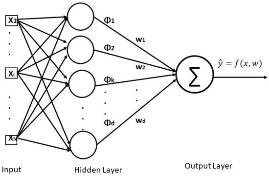
Figure 1.
The conventional multilayer perceptron (MLP) architecture with one hidden layer.
2.1.9. Artificial Neural Network
Similar to MLP, ANN is an interconnected architecture involving multiple neurons, organized into multiple layers. The components of ANN are generally neurons, connections with corresponding weights, and propagation function that can be either forward or backward. ANN architecture can be as shallow as MLP (three layers only) or can be very deep, commonly called Deep Neural Networks. A simple ANN involving one hidden layer uses similar equations like MLP (Equation (15)) for predicting the response variables. For a complex ANN involving several hidden layers, the equation needs to be scaled to accommodate the right number of layers. Training of an ANN involves minimizing the loss function on batches of input examples using gradient descent-like optimization algorithms until the network produces sufficiently accurate predictions. The tuning parameters for the neural network are the size of the hidden layers and the learning rate.
2.2. Evaluation Metrics
Several evaluation metrics such as MSE, R2, RMSE, and MAE were used to evaluate the regression performance. Brief descriptions of these statistical parameters along with their formulations are described below.
2.2.1. Mean Squared Error
The MSE is a statistical measure that calculates the average of the squares of the errors, i.e., the average squared difference between the estimated and actual values. MSE corresponds to the expected value of the squared error loss in the prediction. It can be described as below:
where are observed responses, are estimated responses, and N is the total number of observations.
2.2.2. Coefficient of Determination
The R2 is a statistical measure of how well a regression model fits a set of observations. It is defined as the percentage of the response variable variation that is explained by a regression model. The equation for R2 has the following form:
The R2 value ranges between 0 and 100%. Generally, the higher the R2 the better the model fits the data, i.e., the model can explain most of the variances in the observed responses.
2.2.3. Mean Absolute Error
The MAE is a measure of the difference between two continuous variables. It is an average of absolute errors between the estimated and true responses. It can be defined with the following formula:
where and are the estimated and observed responses, respectively.
2.2.4. Root Mean Square Error
The RMSE is a statistical measure that calculates the standard deviation of the estimation errors. It is a standard way to calculate the error of a model in estimating real-valued responses. The formula for RMSE is as follows:
2.3. Dataset
The experimental data collected from twelve different studies were used for the current investigation. Spherical particles of different sizes were employed for the wet-experiments. The experimental details are summarized in Table 1. The system properties are presented in Table 2. A total of 967 data points was used for the current study. There were six independent or input parameters (ds, ρs, ρl, τo, K, and n) and one dependent or output parameter (Vs). A statistical description of these parameters along with the Reynolds numbers and drag coefficients is presented in Table 3.

Table 1.
Summary of the experimental details.
Table 2.
Summary of datasets used to apply machine-learning algorithms (MLAs).
Table 3.
Statistics of the input parameters.
2.4. ML Modeling
The predictive power of MLA was assessed in the current study by training and testing nine regression models to estimate the settling velocity from six experimental parameters. The MLA modeling included the following steps in successive order: (i) parameter optimization and model selection, (ii) feature importance analysis, and (iii) comprehensive validation of the optimum model [33,34,35,36,37].
2.4.1. Parameter Optimization and Model Selection
The MLA modeling of Vs prediction involved associated parameter optimization on a training set and the final model selection based on the validation using the independent test data points. At first, the datasets extracted from the literature were merged. Next, the merged dataset was split into a training (80%) and a test (20%) subset using random sampling. The training of nine ML models was carried out using the training data points (80%). The test dataset (20%), which can be considered as an independent test set, was withheld for model verification. The statistics of training and test data are presented in Table 4.
Table 4.
Dataset statistics.
A grid search was integrated with a repeated k-fold cross-validation (CV) technique for choosing the most optimized parameters for the ML models and the final model selection [35]. Different hyper-parameters of nine ML models (see Table 5) were optimized such that average prediction error would be minimized on training data. At each fold in the CV, a model was fit on the subsets of training data. The fitted model was then evaluated on the hold-out validation dataset by calculating the RMSE of the prediction. This process was performed k-times with the desired number of repetitions. The model that minimized the average RMSE across the repeated CV was selected as the final model and its corresponding parameters were identified as the optimized ones. In a simple mathematical notation, the following optimization problem was attempted to be solved:
where n is the number of repetitions, k is the number of folds in CV, and RMSEi,j is the root mean square deviation of the predicted response from the actual response (Vs) for j-th fold in i-th iteration of the repeated CV. The algorithm used for model selection in the present study is depicted in Figure 2. Note that, the number of folds in CV (k) and repetition times (N) were considered as 10 in this study. The details of the ML models including R packages, hyper-parameter names, and their optimized values after cross-validated training are reported in Table 5.
Table 5.
The ML models, hyperparameter names, and corresponding optimized values after cross-validated training (the last column includes R packages used for different ML models).
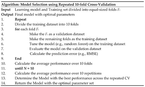
Figure 2.
Algorithmic representation of the repeated k-fold cross-validation (CV) algorithm used for parameter optimization and model selection.
2.4.2. Feature Importance Analysis and Validation
Leave-One-Feature-Out Experiment
While fitting an ML model to the training data, it triggers the question of which variables have the most predictive power or which variables have contributed most in predicting the response variable. The most important variables usually play critical roles in forecasting the response and their values have a significant impact on the predicted outcome. Less relevant features can be eliminated from the model due to their lower impacts, making the model less complex and quicker to train and predict. In practice, two different approaches are adopted to perform feature importance analysis. One is an accuracy-based measure and the other one is a model-based importance measure. In this study, an accuracy-based measure was used to investigate the contribution of different independent parameters in predicting the settling velocity as a response. Accordingly, a leave-one-feature-out experiment was performed [43]. Every single feature was systematically excluded during the model training and the corresponding R2 was calculated. Similar to Reference [1], a relative feature influence (RFI) was introduced in the current study for the convenience of analyzing the feature significance. The formula used to calculate RFI is as follows:
The RFI indicates the relative importance of a feature in predicting the responses (Vs) and is derived using the R2 metrics. The larger the RFI the more significant the feature is.
Leave-one-dataset-out validation
A leave-one-dataset-out experiment was performed to validate the ML models [44]. To conduct this experiment, a series of data augmentation was performed. First, some datasets [15,16,17,18] were merged under one dataset named Rooki (2012). Second, a base training dataset was created by integrating two datasets collected from References [7,11]. These two datasets cover all fluid types used for the current study. It is important to mention that a good amount of base training data associated with each fluid type is needed to produce a better-generalized model. The dry experiment conducted for leave-one-dataset-out validation is demonstrated with an algorithmic flowchart in Figure 3. This validation approach comprising six experiments works through training and testing the model by excluding one dataset at a time.
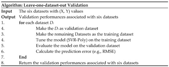
Figure 3.
Algorithmic representation of the leave-one-data-set-out validation involving six datasets.
2.5. Computing Framework
All dry experiments and statistical analyses were performed on a computer with an Intel CORE i7 8th Gen, 2GHz processor, and 8 GB of RAM configuration. All hardware ran under a 64-bit Windows 10 operating system. As a statistical computing framework, R (version 4.0.2) was used for the current study. The prediction time for a data matrix of 200 × 6 dimension was 10 s.
3. Results
3.1. Evaluation of Traditional Modeling Methodologies
The results of traditional implicit and explicit methods are presented in Figure 4, Figure 5 and Figure 6 and Table 6.
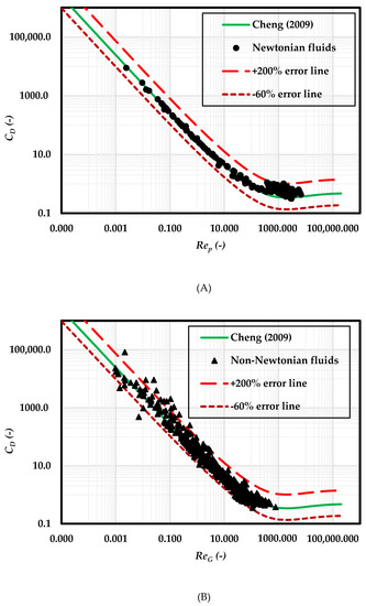
Figure 4.
Predictions of Vs with Cheng [4] model and the associated uncertainty for spherical particles in (A) Newtonian fluids and (B) non-Newtonian fluids.
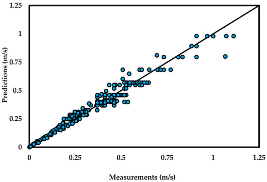
Figure 5.
Predictions of Vs with Ferguson and Church [45] model (fluid rheology: Newtonian; particle shape: spherical).
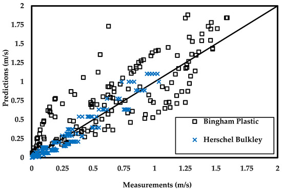
Figure 6.
Predictions of Vs with Okesanya and Kuru [19] model (fluid rheology: non-Newtonian; particle shape: spherical).
Table 6.
The performance of explicit models on the complete dataset.
3.2. MLA Model Evaluation on the Independent Test Set
The performances of nine models in predicting settling velocities for the independent test set are shown in Table 7. Both training and test predictions were evaluated with MAE, RMSE, MSE, and R2 metrics. The performances are also depicted in Figure 7 by plotting the measured values against the predicted values of Vs.
Table 7.
The performances of nine (9) MLA models on training and independent test data.
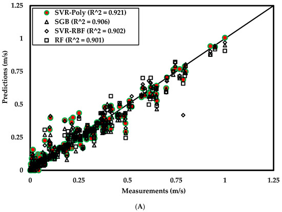
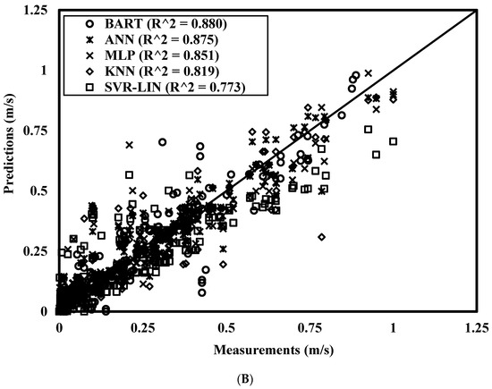
Figure 7.
Performances of the ML models on independent test data: (A) top four models (R2 > 0.9); (B) five low performing models (R2 < 0.9).
3.3. Feature Importance Analysis
The results of the leave-one-feature-out experiment using the best model, SVR-Polynomial Kernel are described in Table 8. The bar plot demonstrating the RFI of six experimental parameters is presented in Figure 8.
Table 8.
The results of the leave-one-feature-out experiment using SVR-Polynomial Kernel.
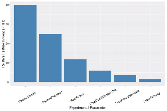
Figure 8.
The relative feature influence of six experimental parameters.
3.4. Leave-One-Dataset-Out Validation
The results of the leave-one-dataset-out validation are presented in Table 8. All the validation experiments were performed using the best performing SVR-polynomial kernel model. The test performances were evaluated using a similar set of evaluation metrics presented in Table 9.
Table 9.
The results of leave-one-dataset-out validation using SVR-Polynomial Kernel.
4. Discussion
4.1. Limitations of Existing Analytical Models
As mentioned earlier, the implicit method of predicting Vs requires using a CD-Rep or CD-ReG correlation to iteratively predict Vs in a Newtonian or non-Newtonian fluid. Although many CD-Rep correlations are available in the literature, all of those were proposed for Newtonian fluids. Originally, Cheng [4] also proposed the correlation for Newtonian rheology. Later, the model was extended by replacing Rep with ReG to different non-Newtonian fluids [7,20,23]. The results of applying this correlation to the current dataset are presented in Figure 4 by plotting CD against Rep and ReG for Newtonian and non-Newtonian fluids, respectively. As expected, the performance of the Cheng correlation is better for Newtonian fluids compared to the non-Newtonian fluids. Most of the measured values collapse over the model curve for Newtonian fluids. For non-Newtonian fluids, the uncertainty of prediction is considerably high. It can be less than −60% and more than 200% for the current dataset. The values of the model coefficients determined empirically for Newtonian fluids do not necessarily account for the variation in viscosity due to shear in non-Newtonian fluids. That is why this kind of correlation is usually validated and modified before using for a non-Newtonian fluid. The associated complexities and uncertainties render predicting Vs using a CD-Rep correlation an inconvenient option for an engineer.
On the other hand, the explicit method involves correlation(s) that can be used to predict Vs directly based on the system properties. The following exemplary models were used for the current study.
4.1.1. Ferguson and Church (FC) Model
Probably, the most accurate explicit model for Vs in Newtonian fluids was developed by Ferguson and Church [45]. Agwu et al. [1] found its performance as comparable to ANN. The FC model (Equation (22)) applies to both laminar and turbulent conditions.
In Equation (22), . and C (-) is a dimensionless constant. The empirical value of C is 0.54 for a spherical particle.
4.1.2. Okesanya and Kuru (OK) Model
It is one of the latest semi-mechanistic models. A series of steps involving conditional calculations are required to be followed to calculate Vs with the OK model. The most important equations are presented as follows.
In Equations (23)–(32),
- : surficial shear stress (Pa)
- : shear velocity (m/s)
- : shear Reynolds number (-)
- : shear generalized Reynolds number (-)
- : model-specific shear Reynolds number (-)
- : relative characteristics shear stress (-): shape factor (-)
Compared to the OK model, the FC model is simple and easy to apply. Its performance in predicting Vs of a spherical particle in a Newtonian fluid is creditable. The agreement between the predicted and measured values is within an acceptable margin of error (Figure 5 and Table 7). However, the model cannot be applied to non-Newtonian fluids in its current form since it requires a constant value for µl. On the other hand, the OK model involves a complex numerical scheme. Although mathematical complexity is not uncommon in modeling a non-Newtonian system, this model is afflicted with a significant limitation. Its application is limited to three rheological models: (i) Herschel Bulkley, (ii) Bingham, and (iii) Casson model. The OK model does not apply to other rheological models, such as power-law and Newton’s law. As shown in Figure 6 and Table 7, the model yields result for the Herschel Bulkley fluids with a practical error limit. However, it fails to do so for Bingham fluids. Thus, similar to other existing models, both of these explicit models are rheology-specific and prone to yielding significant errors.
4.2. Analysis of Current AI Model
A wide range of ML models was selected for modeling the Vs of spherical particles in the present study to develop a generalized model applicable to both Newtonian and non-Newtonian fluids. Parametric regression models, such as SVR, MLP, NN, as well as non-parametric regression models such as KNN, including a comparatively latest approach called Bayesian regression were considered. Among the Bagging and Boosting algorithms, RF and SGB were selected. Table 6 shows the results of ML modeling of the selected regression models through repeated cross-validated training. Among all models, the best model was the SVR-Polynomial kernel (R2 = 0.921) with the optimized values of the parameters, such as degree-d of the kernel as three (3), input scaling parameter as 0.1, and the regularization parameter as 1 (see Table 5). As modeling Vs associates non-linear feature interactions, non-linear ML models were found to have superior performances. In the case of SVR, both RBF and Polynomial kernel map the input space to higher dimensional feature space, and, subsequently, the problem becomes linearly separable into that feature space. The SVR-Polynomial kernel demonstrated better performance than its RBF kernel counterpart in the case of independent test data prediction (see Table 7 and Figure 7). It should be noted that the SVR-Poly yielded comparable values of R2 for both training and test datasets (R2 = 0.931 for training dataset; R2 = 0.921 for test dataset), which demonstrates the robustness of the model. The second-best model was the SGB (R2 = 0.906), which is the stochastic version of the general gradient boosting algorithm. The SVR–RBF along with the RF ranked as the third-best model with an identical R2 value of 0.901 for the test dataset. It is important to observe that both bagging (RF) and boosting (SGB) algorithms with stochastic components were found to perform well either by choosing the best possible random set of predictors (RF) or observations (SGB) for splitting at each node of the regression tree and iteration of minimizing the objective loss function. Both models were able to capture the non-linearity of the data and accurately estimate the actual response.
The SVR-Linear had the least prediction accuracy (R2 = 0.773) among the ML models evaluated for the current study. Given the superior performances of other non-linear kernels in SVR, it is apparent that the original input features are non-linearly separable, and, therefore, SVR-Linear inevitably led to an underfitting of the data. The KNN, as a non-parametric regression method, achieved the second-lowest accuracy with R2 = 0.819. The ANN and MLP achieved the next lower accuracies and exhibited comparable performances with R2 = 0.871 and R2 = 0.851, respectively. This is most likely because both ANN and MLP architectures have similar model complexity with a single hidden layer and different numbers of hidden neurons (20 for ANN and 5 for MLP). The BART could achieve a moderate correlation (R2 = 0.88) with the imposition of regularization on each tree while fitting to a small portion of the training data. It helped to achieve a fairly bias-free prediction when several trees were fitted to the whole set of observations.
The comparative performance analysis of the ML models on independent test data demonstrated all parametric regression models except SVR-Linear to perform better than non-parametric regression models, e.g., KNN-regression. Among the parametric models, the SVR with non-linear kernels was the top performer, while the regression tree with both stochastic and Bayesian components was in the second-best position. The ANN family of regressor models showed ordinary performances that were comparable to the existing ANN models such as [1,14]. The current study proves that MATLAB-based ANN may not provide the best accuracy. Another interesting observation is that the training performances of MLP and SVR-linear are lower than the corresponding independent test performances in terms of all metrics. In the case of MLP, there could be a local minimum that led to the model’s lower performance during training, as this is a usual problem in an NN-like architecture. In the case of SVR-Linear, this is a clear sign of underfitting. In both cases, the models could produce a better prediction for test data points.
One of the important aspects of the current study is a comprehensive feature importance analysis. A leave-one-feature-out strategy was used with six experiments for the purpose. It involved training and testing the model by excluding one feature at a time. The SVR-Polynomial kernel model was used for these experiments because of its superior performance over other ML models on an independent test set. A new set of R2 values were obtained from the leave-one-feature-out experiments. Then, the R2 values obtained before and after excluding each feature were compared. A relative feature importance indicator was used by taking into account the differences observed in R2 values in the presence or absence of a specific feature. The RFI indicates the influence of a feature on the model in relation to the R2 metric. A decreased ranking-order of the features can be obtained based on their RFI values. As shown in Figure 8, the Particle Density and the Particle Diameter are identified as the two most significant features having respective RFI values of 39.6 and 24.8, followed by a decreasing rank-order of Yield Stress, Flow Consistency Index, Flow Behavior Index, and Liquid density. Specifically, the ordering of the features from the highest to lowest ranks is as follows: ρs > ds > τo > K > n > ρl (Figure 8). A similar trend of feature influence was reported in a previous ANN-study [1]. It can be explained with the physics of the settling process. The motion of a particle in a stationary fluid is triggered by the gravitational force (FG). When it is released in the fluid, an acceleration of g (~9.81 m/s2) acts on it. Afterward, the motion of the particle in the fluid actuates a drag force (FD) on itself. Its incremental velocity also intensifies FD. When FD nearly matches FG, an equilibrium condition persists and the particle continues moving at a constant velocity known as the settling velocity. Thus, the opposing forces ensue Vs. The primary force in this process is FG, which is strongly dependent on a spherical particle’s density and size or diameter. The dependency is conceivably stronger on ρs than ds. On the other hand, FD is the secondary force stemmed from the particle motion. It is known to be a strong function of Newtonian fluid viscosity and weakly dependent on ρl. For the non-Newtonian fluids considered in the current study, the rheology was modeled with yield stress, flow consistency index, and flow behavior index. The most important among these parameters is τo as FD cannot be actuated until FG overcomes it. The viscosity of the non-Newtonian fluid is denoted with K while its shear-thinning behavior is signified with n. Understandably, K plays a more significant role than n in the settling process. Thus, the feature-importance, as shown in Figure 8, is in sync with the physics of the particle settling phenomenon. It justifies the utility of the MLA in predicting Vs.
A prediction model can be considered reliable if it generalizes well on completely unseen data that were not used during the training. The leave-one-dataset-out validation (LOOV) examines the generalizability of an MLA. Furthermore, it checks whether training produces a reliable model that could be tested by any other set of experimentally measured values for different types of fluids to predict the corresponding Vs. Although the LOOV experiment performs an objective analysis of the ML-model performance, it is largely absent in the previous ML studies of Vs modeling. Most of the previous studies evaluated their proposed models based on test data that come from the same training distribution. This type of in-distribution evaluation does not inform about the performance of the model when applied to an out-distribution data or a completely new dataset. On the other hand, leave-one-out validation is one of the preferred methods to comprehensively evaluate the generalized performance of ML models [34,35,44]. Agwu et al. [1] attempted to conduct a similar validation. However, their effort was constrained by the number of datasets as they used only two independent datasets. In the current study, the LOOV was used to investigate the generalizability of the MLA that was identified as the optimum choice to model the Vs of a sphere in both Newtonian and non-Newtonian fluids. The dry experiments were conducted by training the SVR-Polynomial kernel model on six datasets. The SVR-Polynomial was selected for the LOOV analysis because of its superior performance over the other ML models in predicting Vs for independent test data. Then, the generalization ability of the model was assessed with four evaluation metrics for each dataset. The SVR-Polynomial kernel model achieves moderate to high performances with the R2 values between 0.65 and 0.91 with an average of 0.78. An analogous analysis was reported in Reference [1]. They applied a total of eighteen (18) explicit models along with their ANN-model to predict the Vs for a specific dataset. A statistical comparison of the predictions produced R2 values in the range of 0.23–0.94 with an average of 0.49. An objective comparison of these independent analyses suggests the current model is capable of producing reliable results for both Newtonian and non-Newtonian fluids within an acceptable error margin.
The open-source statistical computing framework, R, instead of commercial MATLAB, was used in the present study for conducting all ML experiments and performing the statistical analysis. The majority of the previous ANN-based studies utilized MATLAB for developing the prediction models. Compared to MATLAB, R has several advantages: (1) R is completely free of charge, as it is open-source software; (2) it provides numerous packages and built-in functions for ML modeling, fine-tuning the hyper-parameters, data visualization and pre-processing, post-prediction statistical analyses, plotting of result graphs and trends, etc.; (3) R can be used with any operating system; (4) it can be used to develop a web-based DSS that would allow a user to estimate Vs for a given set of process conditions. Furthermore, R is easy to program, well-documented, and evolving continually due to the freelance contributions from the scientific community. Therefore, R is considered a more economic, flexible, and fast-evolving scientific and statistical computing framework compared to MATLAB. It is the industrial choice for data analysis.
As mentioned earlier, the best performing MLA in the current study was SVR-Poly. The upshots of this model are demonstrated in Figure 9 and discussed as follows:
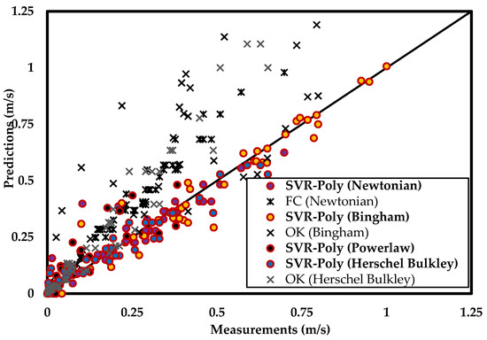
Figure 9.
Comparative performance of the ML model, SVR-Poly, and the traditional explicit models, Ferguson and Church (FC) and Okesanya and Kuru (OK) on the test data.
- (a)
- The SVR-Poly can predict Vs of spherical particles in Newtonian and different varieties of non-Newtonian fluids. Whereas, the FC applies to only Newtonian fluids, and the OK could be applied to two non-Newtonian fluids.
- (b)
- Prediction uncertainties associated with SVR-Poly are comparable for the Newtonian and non-Newtonian rheologies. That is, the ML model is insensitive to fluid rheology. Unlike the traditional models, it is capable of predicting Vs without a bias to the fluid properties.
- (c)
- Prediction accuracy of SVR-Poly is significantly better than the traditional explicit models such as FC and OK models.
5. Conclusions
In the current study, we investigate an ML-based methodology for predicting the settling velocity of spherical particles in the Newtonian fluid and the non-Newtonian fluids following different varieties of rheology such as Power-law, Bingham Plastic, and Herschel Bulkley models. This is because the traditional analytical approach of modeling the velocity, including both explicit and implicit models, cannot provide a generalized solution. Among nine tested ML models, SVR with polynomial kernel provided the best performance in terms of the statistical metrics on an independent test dataset (R2 = 0.92; RMSE = 0.066; MSE = 0.0044; MAE = 0.044). A ten-fold-cross-validation technique was used to ascertain the most suitable model. A comprehensive feature analysis using leave-one-feature-out experiments assured the strong correlation among the parameters selected for modeling and the experimental observations. The correlations were quantified using a relative feature influence indicator. The order of significance for the input parameters was as follows: particle density > particle diameters > yield stress > flow consistency index > flow behavior index > liquid density. Additionally, leave-one-dataset-out validation experiments were conducted to test the reliability of the model for unseen experimental datasets. The model confirmed a reasonable performance in estimating the settling velocity for completely unseen data. It could predict more than 80% of the test data within an error limit of ±20%. The present study provides strong evidence that ML is very effective and accurate as a general predicting tool for the settling velocity of spheres in both Newtonian and non-Newtonian fluids. It can be used as a reliable method in industrial-scale design and operation due to its economical requirements of time and computational resources.
While the current study demonstrates the generalized capability of MLAs in predicting settling velocity, further research is necessary to develop a universal ML model independent of particle shape, particle proximity, fluid rheology, wall proximity, and flow conditions. The works currently underway in this regard include applying the ML models in predicting the hindered settling velocity and developing a smart decision support system.
Author Contributions
Conceptualization, N.H., S.R., and M.A.; methodology, N.H. and S.R.; software, N.H.; validation, N.H. and S.R.; formal analysis, N.H. and S.R.; investigation, N.H., and S.R.; resources, N.H., and S.R.; data curation, M.A.-F. and S.R.; writing—original draft preparation, N.H., S.R., M.A.-F., and M.A.; writing—review and editing, N.H., S.R., M.A.-F., and M.A.; visualization, N.H. and S.R.; supervision, N.H., and S.R.; project administration, N.H., and S.R.; funding acquisition, N.H., S.R., M.A.-F., and M.A. All authors have read and agreed to the published version of the manuscript.
Funding
This research was funded by the Deputyship for Research and Innovation, Ministry of Education, Saudi Arabia, project number IFT20081.
Institutional Review Board Statement
Not applicable.
Informed Consent Statement
Not applicable.
Data Availability Statement
Data presented in this study are openly available in the following references: [2,6,7,11,15,16,17,18,19,20,21,22].
Acknowledgments
The authors extend their appreciation to the Deputyship for Research and Innovation, Ministry of Education, Saudi Arabia. The authors are also grateful to the Deanship of Scientific Research, the College of Computer Science and Information Technology, and the College of Engineering at King Faisal University, Saudi Arabia.
Conflicts of Interest
The authors declare no conflict of interest. The funders had no role in the design of the study; in the collection, analyses, or interpretation of data; in the writing of the manuscript, or in the decision to publish the results.
References
- Agwu, O.E.; Akpabio, J.U.; Dosunmu, A. Artificial Neural network model for predicting drill cuttings settling velocity. Petroleum 2019, in press. [Google Scholar] [CrossRef]
- Arabi, A.S.; Sanders, R.S. Particle terminal settling velocities in non-Newtonian viscoplastic fluids. Can. J. Chem. Eng. 2016, 94, 1092–1101. [Google Scholar] [CrossRef]
- Atapattu, D.; Chhabra, R.; Uhlherr, P. Creeping sphere motion in Herschel-Bulkley fluids: Flow field and drag. J. Nonnewton. Fluid Mech. 1995, 59, 245–265. [Google Scholar] [CrossRef]
- Cheng, N.S. Comparison of formulas for drag coefficient and settling velocity of spherical particles. Powder Technol. 2009, 189, 395–398. [Google Scholar] [CrossRef]
- Elgaddafi, R.; Ahmed, R.; Growcock, F. Settling behavior of particles in fiber-containing Herschel Bulkley fluid. Powder Technol. 2016, 301, 782–793. [Google Scholar] [CrossRef]
- Kelessidis, V.; Mpandelis, G. Measurements and prediction of terminal velocity of solid spheres falling through stagnant pseudoplastic liquids. Powder Technol. 2004, 147, 117–125. [Google Scholar] [CrossRef]
- Rushd, S.; Hassan, I.; Sultan, R.A.; Kelessidis, V.C.; Rahman, A.; Hasan, H.S.; Hasan, A. Terminal settling velocity of a single sphere in drilling fluid. Particul. Sci. Technol. 2018, 37, 943–952. [Google Scholar] [CrossRef]
- Saha, G.; Purohit, N.; Mitra, A. Spherical particle terminal settling velocity and drag in Bingham liquids. Int. J. Miner. Process. 1992, 36, 273–281. [Google Scholar] [CrossRef]
- Stokes, G.G. On the effect of the internal friction of fluids on the motion of pendulums. Trans. Cambridge Philos. Soc. IX. 1851, pp. 8–106. Available online: http://mural.uv.es/daroig/documentos/stokes1850.pdf (accessed on 1 January 2020).
- Turton, R.; Levenspiel, O. A short note on the drag correlation for spheres, Powder Technol. Powder Technol. 1986, 47, 83–86. [Google Scholar] [CrossRef]
- Wilson, K.; Horsley, R.; Kealy, T.; Reizes, J.; Horsley, M. Direct prediction of fall velocities in non-Newtonian materials. Int. J. Miner. Process. 2003, 71, 17–30. [Google Scholar] [CrossRef]
- Machac, I.; Ulbrichova, I.; Elson, T.; Cheesman, D. Fall of spherical particles through non-Newtonian suspensions. Chem. Eng. Sci. 1995, 50, 3323–3327. [Google Scholar] [CrossRef]
- Agwu, O.E.; Akpabio, J.U.; Alabi, S.B.; Dosunmu, A. Settling velocity of drill cuttings in drilling fluids: A review of experimental, numerical simulations and artificial intelligence studies. Powder Technol. 2018, 339, 728–746. [Google Scholar] [CrossRef]
- Rooki, R.; Ardejani, F.D.; Moradzadeh, A.; Kelessidis, V.C.; Nourozi, M. Prediction of terminal velocity of solid spheres falling through Newtonian and non-Newtonian pseudoplastic power law fluid using artificial neural network. Int. J. Miner. Process. 2012, 110, 53–61. [Google Scholar] [CrossRef]
- Ford, J.T.; Oyeneyin, M.B. The formulation of milling fluids for efficient hole cleaning: An experimental investigation. In Proceedings of the European Petroleum Conference, London, UK, 25–27 October 1994. [Google Scholar] [CrossRef]
- Kelessidis, V.C. An explicit equation for the terminal velocity of solid spheres falling in pseudoplastic liquids. Chem. Eng. Sci. 2004, 59, 4437–4447. [Google Scholar] [CrossRef]
- Miura, H.; Takahashi, T.; Ichikawa, J.; Kawase, Y. Bed expansion in liquid–solid two-phase fluidized beds with Newtonian and non-Newtonian fluids over the wide range of Reynolds numbers. Powder Technol. 2001, 117, 239–246. [Google Scholar] [CrossRef]
- Pinelli, D.; Magelli, F. Solids settling velocity and distribution in slurry reactors with dilute pseudoplastic suspensions. Ind. Eng. Chem. Res. 2001, 40, 4456–4462. [Google Scholar] [CrossRef]
- Okesanya, T.; Kuru, E.A. New generalized model for predicting particle settling velocity in viscoplastic fluids. In Proceedings of the SPE Annual Technical Conference and Exhibition, Society of Petroleum Engineers, Calgary, AB, Canada, 30 September–2 October 2019. [Google Scholar] [CrossRef]
- Okesanya, T.; Kuru, E.; Sun, Y.A. New generalized model for predicting the drag coefficient and the settling velocity of rigid spheres in viscoplastic fluids. SPE J. 2020. [Google Scholar] [CrossRef]
- Shahi, S. An Experimental Investigation of Settling Velocity of Spherical and Industrial Sand Particles in Newtonian and Non-Newtonian Fluids Using Particle Image Shadowgraph. Master’s Thesis, University of Alberta, Edmonton, AB, Canada, 2014. [Google Scholar] [CrossRef]
- Song, X.; Xu, Z.; Li, G.; Pang, Z.; Zhu, Z. A new model for predicting drag coefficient and settling velocity of spherical and non-spherical particle in Newtonian fluid. Powder Technol. 2017, 321, 242–250. [Google Scholar] [CrossRef]
- Xu, Z.; Song, X.; Zhu, Z. Development of elastic drag coefficient model and explicit terminal settling velocity equation for particles in viscoelastic fluids. SPE J. 2020. [Google Scholar] [CrossRef]
- Zhu, Z.; Wang, H.; Peng, D.; Dou, J. Modelling the hindered settling velocity of a falling particle in a particle-fluid mixture by the Tsallis entropy theory. Entropy 2019, 21, 55. [Google Scholar] [CrossRef]
- Zhang, Y.; Ban, X.; Wang, X.; Liu, X. A symmetry particle method towards implicit non-Newtonian fluids. Symmetry 2017, 9, 26. [Google Scholar] [CrossRef]
- Riaz, A.; Bhatti, M.M.; Ellahi, R.; Zeeshan, A.M.; Sait, S. Mathematical analysis on an asymmetrical wavy motion of blood under the influence entropy generation with convective boundary conditions. Symmetry 2020, 12, 102. [Google Scholar] [CrossRef]
- Wang, X.; Ban, X.; He, R.; Wu, D.; Liu, X.; Xu, Y. Fluid-solid boundary handling using pairwise interaction model for non-Newtonian fluid. Symmetry 2018, 10, 94. [Google Scholar] [CrossRef]
- Golshan, A.; Gohari, S.; Ayob, A. Multi-objective optimisation of electrical discharge machining of metal matrix composite Al/SiC using non-dominated sorting genetic algorithm. Int. J. Mechatron. Manuf. Syst. 2012, 5, 385–398. [Google Scholar] [CrossRef]
- Golshan, A.; Ghodsiyeh, D.; Gohari, S.; Amran, A.; Baharudin, B.T. Computational inteligence in optimization of machining operation parameters of ST-37 steel. Appl. Mech. Mater. 2012, 248, 456–461. [Google Scholar] [CrossRef]
- Clarke, S.M.; Griebsch, J.H.; Simpson, T.W. Analysis of support vector regression for approximation of complex engineering analyses. J. Mech. Des. 2005, 127, 1077–1087. [Google Scholar] [CrossRef]
- Ladický, L.U.; Jeong, S.; Solenthaler, B.; Pollefeys, M.; Gross, M. Data-driven fluid simulations using regression forests. ACM TOG 2015, 34, 1–9. [Google Scholar] [CrossRef]
- Patri, A.; Patnaik, Y. Random forest and stochastic gradient tree boosting based approach for the prediction of airfoil self-noise. Procedia Comput. Sci. 2015, 46, 109–121. [Google Scholar] [CrossRef]
- Wang, Z.; Liu, Q.; Liu, Y. Mapping landslide susceptibility using machine learning algorithms and GIS: A case study in Shexian County, Anhui Province, China. Symmetry 2020, 12, 1954. [Google Scholar] [CrossRef]
- Chen, C.; Deng, J.; Yu, X.; Wu, F.; Men, K.; Yang, Q.; Zhu, Y.; Liu, X.; Jiang, Q. Identification of novel inhibitors of DDR1 against idiopathic pulmonary fibrosis by integrative transcriptome meta-analysis, computational and experimental screening. Mol. Biosyst. 2016, 12, 1540–1551. [Google Scholar] [CrossRef]
- Menden, K.; Marouf, M.; Oller, S.; Dalmia, A.; Magruder, D.S.; Kloiber, K.; Heutink, P.; Bonn, S. Deep learning–based cell composition analysis from tissue expression profiles. Sci. Adv. 2020, 6, eaba2619. [Google Scholar] [CrossRef] [PubMed]
- Achirul Nanda, M.; Boro Seminar, K.; Nandika, D.; Maddu, A. A Comparison study of Kernel functions in the support vector machine and its application for Termite detection. Information 2018, 9, 5. [Google Scholar] [CrossRef]
- Gutiérrez-Esparza, G.O.; Infante Vázquez, O.; Vallejo, M.; Hernández-Torruco, J. Prediction of metabolic syndrome in a Mexican population applying machine learning algorithms. Symmetry 2020, 12, 581. [Google Scholar] [CrossRef]
- Hill, J.; Linero, A.; Murray, J. Bayesian additive regression trees: A review and look forward. Annu. Rev. Stat. Appl. 2020, 7, 251–278. [Google Scholar] [CrossRef]
- Pereira Härter, F.; Fraga de Campos Velho, H. Multilayer perceptron neural network in a data assimilation scenario. Eng. Appl. Comput. Fluid Mech. 2010, 4, 237–245. [Google Scholar] [CrossRef]
- Friedman, J.H. Stochastic gradient boosting. CSDA 2002, 38, 367–378. [Google Scholar] [CrossRef]
- Chipman, H.A.; George, E.I.; McCulloch, R.E. BART: Bayesian additive regression trees. Ann. Appl. Stat. 2010, 4, 266–298. [Google Scholar] [CrossRef]
- Rodriguez, J.D.; Perez, A.; Lozano, J.A. Sensitivity analysis of k-fold cross validation in prediction error estimation. IEEE PAMI 2009, 32, 569–575. [Google Scholar] [CrossRef]
- Cawley, G.C.; Talbot, N.L. Efficient leave-one-out cross-validation of kernel fisher discriminant classifiers. Pattern Recognit. 2003, 136, 2585–2592. [Google Scholar] [CrossRef]
- Fushiki, T. Estimation of prediction error by using K-fold cross-validation. Stat. Comput. 2011, 21, 137–146. [Google Scholar] [CrossRef]
- Ferguson, R.I.; Church, M. A simple universal equation for grain settling velocity. J. Sediment. Res. 2004, 74, 933–937. [Google Scholar] [CrossRef]
Publisher’s Note: MDPI stays neutral with regard to jurisdictional claims in published maps and institutional affiliations. |
© 2021 by the authors. Licensee MDPI, Basel, Switzerland. This article is an open access article distributed under the terms and conditions of the Creative Commons Attribution (CC BY) license (http://creativecommons.org/licenses/by/4.0/).