Local and Nonlocal Reductions of Two Nonisospectral Ablowitz-Kaup-Newell-Segur Equations and Solutions

Abstract

In this paper, local and nonlocal reductions of two nonisospectral Ablowitz-Kaup-Newell-Segur equations, the third order nonisospectral AKNS equation and the negative order nonisospectral AKNS equation, are studied. By imposing constraint conditions on the double Wronskian solutions of the aforesaid nonisospectral AKNS equations, various solutions for the local and nonlocal nonisospectral modified Korteweg-de Vries equation and local and nonlocal nonisospectral sine-Gordon equation are derived, including soliton solutions and Jordan block solutions. Dynamics of some obtained solutions are analyzed and illustrated by asymptotic analysis.

1. Introduction

The study of the nonisospectral integrable systems has become in recent years a focus of attention within the theory of integrable systems. Compared with the isospectral integrable equations, the nonisospectral integrable equations [1,2,3] are usually used to describe solitary waves in nonuniform media and have time-varying solitary wave solutions. In general, depending on the linear problem, a nonisospectral integrable hierarchy can be derived from the Lax equation, zero curvature equation, or in the frame of Kac-Moody algebra, and so forth [4,5,6]. In Reference [7], Ablowitz, Kaup, Newell and Segur proposed a spectral problem, named Ablowitz-Kaup-Newell-Segur (AKNS) spectral problem,

$$\begin{array}{cc}\hfill & {\Phi }_x=M\Phi ,M=\left(\begin{array}{cc}\lambda & u\\ v& -\lambda \end{array}\right),\Phi =\left(\begin{array}{c}{\Phi }_1\\ {\Phi }_2\end{array}\right),\hfill \end{array}$$

(1)

with spectral parameter $\lambda$ and potentials $u=u(x,t)$ and $v=v(x,t)$, which provides integrable backgrounds for several nonlinear systems with physical significance, including the Korteweg-de Vries (KdV) equation, the modified Korteweg-de Vries (mKdV) equation, the sine-Gordon (sG) equation, and the nonlinear Schrödinger (NLS) equation. When ${\lambda }_t\ne 0$, by imposing time evolution

$$\begin{array}{c}\hfill {\Phi }_t=N\Phi ,N=\left(\begin{array}{cc}A& B\\ C& -A\end{array}\right),\end{array}$$

(2)

then in terms of the compatibility condition ${\Phi }_{xt}={\Phi }_{tx}$, a nonisospectral AKNS hierarchy can be given. In the nonisospectral AKNS hierarchy, there are two types of hierarchy, which are positive order nonisospectral AKNS hierarchy and negative order nonisospectral AKNS hierarchy. The positive one corresponds to ${\lambda }_t\propto {\lambda }^n$ with $n\in {\mathbb{Z}}^{+}$ and the negative one corresponds to ${\lambda }_t\propto {\lambda }^n$ with $n\in {\mathbb{Z}}^{-}$. The nonisospectral AKNS hierarchy was investigated by Chen et al. from the aspect of Lie algebraic structure [8] and then studied by Ma on the Lax representations and Lax operator algebras [9]. Besides, Bäcklund transformation and Darboux transformation were also considered for the nonisospectral AKNS hierarchy [10,11]. For the positive order nonisospectral AKNS hierarchy, one of the prototypical members is the third order nonisospectral AKNS equation, which reads

$$\begin{array}{c}{u}_t=x(u_{xxx}-6uv{u}_x)+3(u_{xx}-2u^{2}v)-2u_x{\partial }^{-1}uv+4u{\partial }^{-1}u{v}_x,\hfill \end{array}$$

(3a)

$$\begin{array}{c}{v}_t=x(v_{xxx}-6uv{v}_x)+3(v_{xx}-2u{v}^2)-2v_x{\partial }^{-1}uv+4v{\partial }^{-1}{u}_{x}v.\hfill \end{array}$$

(3b)

For the negative order nonisospectral AKNS hierarchy, the typical member is the negative order nonisospectral AKNS equation, that is,

$$\begin{array}{c}{u}_{xt}+2u{\partial }^{-1}{\left(uv\right)}_t=xu,\hfill \end{array}$$

(4a)

$$\begin{array}{c}{v}_{xt}+2v{\partial }^{-1}{\left(uv\right)}_t=xv.\hfill \end{array}$$

(4b)

In Equations (3) and (4), ${\partial }^{-1}=\frac{1}{2}\left({\int }_{-\infty }^x-{\int }_x^{+\infty }\right)·dx$. Up to now, several works have been done to search for exact solutions of the nonisospectral AKNS type equations. Soliton solutions for the positive order nonisospectral AKNS hierarchy were obtained through the inverse scattering transform [12]. In References [13,14], Hirota’s bilinear method and double Wronskian technique were used to construct soliton solutions for the second order nonisospectral AKNS equation and the third order nonisospectral AKNS Equation (3). Subsequently, these two methods were applied to investigating soliton solutions of a negative order nonisospectral AKNS equation [15].

The systems with “parity-time symmetry” have drawn much attention in recent years, particularly from the perspective of complete integrability and exact solutions. The “parity-time symmetric” systems are important as theoretically the self-induced potential is invariant. The study of these systems dates back to the pioneering work of Ablowitz and Musslimani [16], where an integrable nonlocal NLS equation was proposed. The corresponding wave propagation in symmetric waveguides and photonic lattices has been demonstrated experimentally. By introducing generalization to the AKNS spectral problem (1) and considering simple symmetry reductions, several reverse space-time and reverse time nonlocal nonlinear integrable equations have been introduced [17]. These include the reverse space-time, and in some cases reverse time, nonlocal NLS, mKdV, sG, (1 + 1) and (2 + 1) dimensional three-wave interaction, derivative NLS, “loop soliton” and Davey-Stewartson equations. The nonlocal integrable systems can be usually applied to describe the two-place (Alice-Bob) physics or multi-place physics (see References [18,19,20]). In Reference [21], Yang and Yang systematically studied the transformations between some nonlocal and local integrable equations. Examples include nonlocal NLS and Davey-Stewartson equations, a nonlocal derivative NLS equation, the reverse space-time complex mKdV equation, and so forth. To date, a variety of nonlocal integrable systems have been investigated, such as multidimensional nonlocal integrable system [22], semi-discrete and discrete nonlocal integrable system [23,24], nonlocal integrable hierarchy [25], and so on. With regards to solutions for nonlocal integrable systems, some approaches have been developed in recent years, such as inverse scattering transform [26], Darboux transformation [27,28,29,30,31], the bilinear method [32,33,34,35] and the Cauchy matrix approach [36].

In spite of many works on isospectral nonlocal integrable systems, there was little work on the nonisospectral nonlocal integrable systems. Very recently, from one of the second order nonisospectral AKNS equations, Liu, Wu and Zhang [37] investigated a nonlocal Gross-Pitaevskii equation and constructed its 1-soliton solution, 2-soliton solutions and Jordan block solutions. Feng and Zhao [38] studied the nonlocal reductions of another second order nonisospectral AKNS equation. As a result, a reverse time nonlocal NLS equation and a reverse space nonlocal NLS equation were derived. Soliton solutions of the resulting nonlocal equations and their dynamics were presented.

In this paper, we are interested in the nonlocal versions of the nonisospectral mKdV-I equation

$$\begin{array}{c}\hfill u_t=x(u_{xxx}-6\delta u^2{u}_x)+3(u_{xx}-2\delta u^3)-2\delta u_x{\partial }^{-1}{u}^2+4\delta u{\partial }^{-1}u{u}_x,\end{array}$$

(5)

and the nonisospectral mKdV-II equation

$$\begin{array}{c}\hfill u_t=x(u_{xxx}-6\delta u{u}^{*}{u}_x)+3(u_{xx}-2\delta u^2{u}^{*})-2\delta u_x{\partial }^{-1}u{u}^{*}+4\delta u{\partial }^{-1}u{u}_x^{*}.\end{array}$$

(6)

Here and hereafter $\delta =\pm 1$ and asterisk denotes the complex conjugate. Furthermore, we will study the nonlocal versions of the nonisospectral sG-I equation

$$\begin{array}{c}\hfill u_{xt}+2\delta u{\partial }^{-1}{\left(u^2\right)}_t=xu,\end{array}$$

(7)

and the nonisospectral sG-II equation

$$\begin{array}{c}\hfill u_{xt}+2\delta u{\partial }^{-1}{\left(u{u}^{*}\right)}_t=xu.\end{array}$$

(8)

We will take into account of bilinearization-reduction technique and derive double Wronskian solutions for the local and nonlocal nonisospectral mKdV equations and the local and nonlocal nonisospectral sG equations. In what follows, we call Equation (3) by nAKNS(3), respectively, Equation (4) by nAKNS(-1) for short. In addition, we name Equations (5)–(8) nmKdV-I, nmKdV-II, nsG-I and nsG-II, respectively.

The outline of this paper is as follows. In Section 2, we recall the Lax representations of the Equations (3) and (4). In Section 3 and Section 4, we present the real local and nonlocal reductions and the complex local and nonlocal reductions of the Equations (3) and (4), respectively. Soliton solutions and Jordan block solutions for the resulting equations are derived from the solutions of the nAKNS(3) Equation (3) and the nAKNS(-1) Equation (4) by considering suitable constraints on the elements of the double Wronski determinant. Dynamics of some obtained solutions are analyzed and illustrated by asymptotic analysis. Section 5 is devoted to the conclusions.

2. Lax Representations of the Equations (3) and (4)

In this section, we briefly recall the Lax representations of the Equations (3) and (4). For the details one can refer to References [15,39]. In what follows, we appoint that $K^T$ represents the transpose of matrix K.

We now pay attention to the spectral problem (1) and time evolution (2). Their compatibility condition ${\Phi }_{xt}={\Phi }_{tx}$ or moreover zero curvature equation $M_t-N_x+[M,N]=0$ gives rise to

$$\begin{array}{c}A={\partial }^{-1}(v,u)\left(\begin{array}{c}-B\\ C\end{array}\right)-{\lambda }_{t}x+A_0,\hfill \end{array}$$

(9a)

$$\begin{array}{c}{\left(\begin{array}{c}u\\ v\end{array}\right)}_t=L\left(\begin{array}{c}-B\\ C\end{array}\right)-2\lambda \left(\begin{array}{c}-B\\ C\end{array}\right)-2A_0\left(\begin{array}{c}-u\\ v\end{array}\right)+2{\lambda }_t\left(\begin{array}{c}-xu\\ xv\end{array}\right),\hfill \end{array}$$

(9b)

where $A_0$ is a constant and

$$\begin{array}{c}\hfill L=\left(\begin{array}{cc}-\partial & 0\\ 0& \partial \end{array}\right)+2\left(\begin{array}{c}u\\ -v\end{array}\right){\partial }^{-1}(v,u).\end{array}$$

(10)

Setting ${\lambda }_t=\frac{1}{2}{\left(2\lambda \right)}^n$, $A_0=0$ and expanding ${(B,C)}^T$ into polynomial as

$$\begin{array}{c}\hfill \left(\begin{array}{c}B\\ C\end{array}\right)=\sum _{j=1}^n\left(\begin{array}{c}{b}_j\\ c_j\end{array}\right){\lambda }^{n-j},\end{array}$$

(11)

by imposing some special choices on ${(b_j,c_j)}^T$, from (9b) one can derive the positive order nonisospectral AKNS hierarchy

$$\begin{array}{c}\hfill {\left(\begin{array}{c}u\\ v\end{array}\right)}_t=L^n\left(\begin{array}{c}-xu\\ xv\end{array}\right),(n=0,1,2,\cdots ).\end{array}$$

(12)

In particular, for $n=3$ one can derive the nAKNS(3) Equation (3) with

$$\begin{array}{c}A=-4x{\lambda }^3+2\lambda (xuv+{\partial }^{-1}uv)+(x+{\partial }^{-1})(u{v}_x-u_{x}v),\hfill \end{array}$$

(13a)

$$\begin{array}{c}B=4xu{\lambda }^2-2(x{u}_x+u)\lambda +2u_x+x(u_{xx}-2u^{2}v)-2u{\partial }^{-1}uv,\hfill \end{array}$$

(13b)

$$\begin{array}{c}C=4xv{\lambda }^2+2(x{v}_x+v)\lambda +2v_x+x(v_{xx}-2u{v}^2)-2v{\partial }^{-1}uv.\hfill \end{array}$$

(13c)

Setting ${\lambda }_t=\frac{1}{2}{\left(2\lambda \right)}^{-n},A_0=0$ and expanding ${(B,C)}^T$ into

$$\begin{array}{c}\hfill \left(\begin{array}{c}B\\ C\end{array}\right)=\sum _{j=1}^n\left(\begin{array}{c}{\overline{b}}_j\\ {\overline{c}}_j\end{array}\right){\lambda }^{j-n-1},\end{array}$$

(14)

then by analogous analysis one can obtain the negative order nonisospectral AKNS hierarchy

$$\begin{array}{c}\hfill {\left(\begin{array}{c}u\\ v\end{array}\right)}_t=L^{-n}\left(\begin{array}{c}-xu\\ xv\end{array}\right),(n=1,2,\cdots ),\end{array}$$

(15)

where a formal expression of $L^{-1}$ was given in Reference [40] (see also Reference [41]). We rewrite (15) as

$$\begin{array}{c}\hfill L^n{\left(\begin{array}{c}u\\ v\end{array}\right)}_t=\left(\begin{array}{c}-xu\\ xv\end{array}\right),(n=1,2,\cdots ),\end{array}$$

(16)

and know that the first member $(n=1)$ is (4). The expressions of A, B and C in (2) for the Equation (4) read

$$\begin{array}{c}\hfill A=-\frac{1}{2\lambda }{\partial }^{-1}{\left(uv\right)}_t-\frac{x}{4\lambda },B=\frac{u_t}{2\lambda },C=-\frac{v_t}{2\lambda }.\end{array}$$

(17)

3. Local and Nonlocal Reductions of the nAKNS(3) Equation (3)

In this section, we shall consider the local and nonlocal reductions of the nAKNS(3) Equation (3). As a result, nonlocal version of nmKdV-I Equation (5) and nmKdV-II Equation (6) will be studied. The approach is bilinearization-reduction technique, which is originally due to Chen, Deng, Lou and Zhang (see Reference [34]). We first recall the bilinearization and double Wronskian solutions to the nAKNS(3) Equation (3) (see Reference [14]) and then investigate its real local and nonlocal reductions and complex local and nonlocal reductions. Moreover, soliton solutions and Jordan block solutions, as well as the dynamics will be presented. For notational brevity, in what follows, we omit the index of each unit matrix I to indicate its size.

3.1. Double Wronskian Solutions

Through the dependent variable transformations

$$\begin{array}{c}\hfill u=\frac{g}{f},v=\frac{h}{f},\end{array}$$

(18)

the nAKNS(3) Equation (3) is written as the following bilinear form

$$\begin{array}{c}{D}_{t}g·f=(x{D}_x^3+3D_x^2)g·f+2D_{x}g·f_x+2gs,\hfill \end{array}$$

(19a)

$$\begin{array}{c}{D}_{t}h·f=(x{D}_x^3+3D_x^2)h·f+2D_{x}h·f_x-2hs,\hfill \end{array}$$

(19b)

$$\begin{array}{c}{D}_x^{2}f·f=-2gh,\hfill \end{array}$$

(19c)

$$\begin{array}{c}{D}_{x}h·g=D_{x}s·f,\hfill \end{array}$$

(19d)

where s is an auxiliary variable and D is the well-known Hirota’s bilinear operator [42] defined by

$$\begin{array}{c}\hfill D_t^m{D}_x^{n}g·f={({\partial }_t-{\partial }_{t^{\prime }})}^m{({\partial }_x-{\partial }_{x^{\prime }})}^{n}g(t,x)f(t^{\prime },x^{\prime }){|}_{t^{\prime }=t,x^{\prime }=x}.\end{array}$$

The double Wronskian is a determinant of a double Wronski matrix composed by two basic column vectors, that is,

$$\begin{array}{c}\hfill |\varphi ,{\partial }_x\varphi ,\dots ,{\partial }_x^{\left(n\right)}\varphi ;\psi ,{\partial }_x\psi ,\dots ,{\partial }_x^{\left(m\right)}\psi |,\end{array}$$

(20)

where the basic column vectors are

$$\begin{array}{c}\hfill \varphi ={({\varphi }_1,{\varphi }_2,\dots ,{\varphi }_{n+m+2})}^T,\psi ={({\psi }_1,{\psi }_2,\dots ,{\psi }_{n+m+2})}^T.\end{array}$$

(21)

Following the standard shorthand notation given in Reference [43], the $(n+m+2)$th-order double Wronskian (20) is indicated by

$$\begin{array}{c}\hfill |{\widehat{\varphi }}^{\left(n\right)};{\widehat{\psi }}^{\left(m\right)}|.\end{array}$$

(22)

Double Wronski determinant solutions of bilinear form (19) are presented by the following theorem.

Theorem 1. 

The double Wronski determinants

$$\begin{array}{c}f(\varphi ,\psi )=|{\widehat{\varphi }}^{\left(n\right)};{\widehat{\psi }}^{\left(m\right)}|,g(\varphi ,\psi )=2|{\widehat{\varphi }}^{(n+1)};{\widehat{\psi }}^{(m-1)}|,h(\varphi ,\psi )=-2|{\widehat{\varphi }}^{(n-1)};{\widehat{\psi }}^{(m+1)}|,\hfill \end{array}$$

(23a)

$$\begin{array}{c}s(\varphi ,\psi )=2\left(\right|{\widehat{\varphi }}^{\left(n\right)};{\widehat{\psi }}^{(m-2)},{\psi }^{\left(m\right)},{\psi }^{(m+1)}|-|{\widehat{\varphi }}^{(n-2)},{\varphi }^{\left(n\right)},{\varphi }^{(n+1)};{\widehat{\psi }}^{\left(m\right)}|\hfill \\ +|{\widehat{\varphi }}^{(n-1)},{\varphi }^{(n+2)};{\widehat{\psi }}^{\left(m\right)}|-|{\widehat{\varphi }}^{\left(n\right)};{\widehat{\psi }}^{(m-1)},{\psi }^{(m+2)}\left|\right),\hfill \end{array}$$

(23b)

solve the bilinear system (19), provided that ϕ and ψ satisfy the following conditions

$$\begin{array}{cc}\hfill & {\varphi }_x=-\frac{1}{2}\Lambda \left(t\right)\varphi ,{\psi }_x=\frac{1}{2}\Lambda \left(t\right)\psi ,\hfill \end{array}$$

(24a)

$$\begin{array}{cc}\hfill & {\varphi }_t=4x{\varphi }_{xxx}+(6-4n){\varphi }_{xx},{\psi }_t=4x{\psi }_{xxx}+(6-4m){\psi }_{xx},\hfill \end{array}$$

(24b)

respectively, where $\Lambda \left(t\right)$ is an $(n+m+2)\times (n+m+2)$ matrix satisfying ${\Lambda }_t\left(t\right)={\Lambda }^3\left(t\right)$.

The proof of the above theorem is similar to the one given in Reference [14], where in that case $\Lambda \left(t\right)$ is diagonal form. To proceed, let us consider the condition equation set (24), which implies

$$\begin{array}{c}\hfill \varphi ={\left(\frac{1}{\sqrt{2}}\Lambda \left(t\right)\right)}^{\frac{3}{2}-n}{e}^{-\frac{1}{2}\Lambda \left(t\right)x}\alpha ,\psi ={\left(\frac{1}{\sqrt{2}}\Lambda \left(t\right)\right)}^{\frac{3}{2}-m}{e}^{\frac{1}{2}\Lambda \left(t\right)x}\beta ,\end{array}$$

(25a)

where

$$\begin{array}{c}\hfill \alpha ={({\alpha }_1,{\alpha }_2,\dots ,{\alpha }_{n+m+2})}^T,\beta ={({\beta }_1,{\beta }_2,\dots ,{\beta }_{n+m+2})}^T,\end{array}$$

(25b)

are two constant column vectors.

3.2. Real Local and Nonlocal Reductions

In this subsection, we will apply the reduction technique to constructing solutions for the nonlocal version of nmKdV-I Equation (5). The idea is that we impose suitable constraints on the pair $(\varphi ,\psi )$ in the double Wronskian so that (18) coincides with the reduction (26).

3.2.1. Reduction Procedure

Let us now consider the real local and nonlocal reductions of the nAKNS(3) Equation (3). We set

$$\begin{array}{c}\hfill v\left(x\right)=\delta u\left(\sigma x\right),\sigma =\pm 1.\end{array}$$

(26)

Applying (26) to (3), we obtain

$$\begin{array}{c}\hfill u_t=x(u_{xxx}-6\delta uu\left(\sigma x\right)u_x)+3(u_{xx}-2\delta u\left(\sigma x\right)u^2)-2\delta u_x{\partial }^{-1}uu\left(\sigma x\right)+4\delta u{\partial }^{-1}u{u}_x\left(\sigma x\right).\end{array}$$

(27)

When $\sigma =1$, Equation (27) is nothing but exactly the nmKdV-I Equation (5). When $\sigma =-1$, Equation (27) is referred to as reverse space nmKdV-I equation. It is worthy to note that the nonlocal reduction of nAKNS(3) Equation (3) is different from the nonlocal reduction of the third order isospectral AKNS equation

$$\begin{array}{cc}\hfill & u_t=u_{xxx}-6uv{u}_x,\hfill \end{array}$$

(28a)

$$\begin{array}{cc}\hfill & v_t=v_{xxx}-6uv{v}_x.\hfill \end{array}$$

(28b)

Equation (28) admits reverse space-time reduction, and the resulting equation is reverse space-time mKdV equation (cf. Reference [17]). While here for the nAKNS(3) Equation (3), the nonlocal reduction is reverse space form. This maybe the effect of the coefficient x in the nAKNS(3) Equation (3). We observe that Equation (27) is preserved under transformation $u\to -u$. Besides, Equation (27) with $(\sigma ,\delta )=(\pm 1,1)$ and with $(\sigma ,\delta )=(\pm 1,-1)$ can be transformed from each other by taking $u\to \pm iu$.

We now consider the real local and nonlocal reductions on the level of the exact solutions of the nAKNS(3) Equation (3). For this purpose, we take $m=n$. Double Wronskian solutions to Equation (27) can be summarized in the following theorem.

Theorem 2.

Exact solutions of the local and nonlocal nmKdV-I Equation (27) are given by

$$\begin{array}{c}\hfill u=\frac{g}{f},f=|{\widehat{\varphi }}^{\left(n\right)};{\widehat{\psi }}^{\left(n\right)}|,g=2|{\widehat{\varphi }}^{(n+1)};{\widehat{\psi }}^{(n-1)}|,\end{array}$$

(29)

in which ϕ and ψ are the $2(n+1)$th order column vectors defined by (25), and satisfy the following relation

$$\begin{array}{c}\hfill \psi \left(x\right)={(-\sigma )}^{\frac{3}{2}-n}T\varphi \left(\sigma x\right),\end{array}$$

(30)

where $T\in {\mathbb{C}}^{2(n+1)\times 2(n+1)}$ is a constant matrix satisfying

$$\begin{array}{c}\hfill \Lambda \left(t\right)T+\sigma T\Lambda \left(t\right)=0,T^2=-\delta I,\end{array}$$

(31)

and we require $\beta =T\alpha$.

Proof. 

Let us first consider the relation (30). In terms of the Equations (31), we have

$$\begin{array}{cc}\hfill \psi \left(x\right)& ={\left(\frac{1}{\sqrt{2}}\Lambda \left(t\right)\right)}^{\frac{3}{2}-n}{e}^{\frac{1}{2}\Lambda \left(t\right)x}\beta ,\hfill \\ \hfill & ={\left(-\frac{1}{\sqrt{2}}\sigma T\Lambda \left(t\right)T^{-1}\right)}^{\frac{3}{2}-n}{e}^{-\frac{1}{2}(\sigma T\Lambda \left(t\right)T^{-1})x}\beta \hfill \\ \hfill & ={(-\sigma )}^{\frac{3}{2}-n}T{\left(\frac{1}{\sqrt{2}}\Lambda \left(t\right)\right)}^{\frac{3}{2}-n}{e}^{-\frac{1}{2}\sigma \Lambda \left(t\right)x}\alpha \hfill \\ \hfill & ={(-\sigma )}^{\frac{3}{2}-n}T\varphi \left(\sigma x\right).\hfill \end{array}$$

(32)

We now apply (30) to considering the relations among variables f, g and h. To achieve this, we introduce a notation

$$\begin{array}{c}\hfill {\widehat{\varphi }}^{\left(s\right)}{\left(ax\right)}_{\left[bx\right]}={(\varphi \left(ax\right),{\partial }_{bx}\varphi \left(ax\right),\dots ,{\partial }_{bx}^s\varphi \left(ax\right))}_{2(n+1)\times 2(s+1)},\end{array}$$

(33)

where a, b = $\pm 1$. Following this notation, we can rewrite variables f, g and h as

$$\begin{array}{cc}\hfill & f=|{\widehat{\varphi }}^{\left(n\right)};{\widehat{\psi }}^{\left(n\right)}|=|{\widehat{\varphi }}^{\left(n\right)}{\left(x\right)}_{\left[x\right]};{(-\sigma )}^{\frac{3}{2}-n}T{\widehat{\varphi }}^{\left(n\right)}{\left(\sigma x\right)}_{\left[x\right]}|,\hfill \end{array}$$

(34a)

$$\begin{array}{cc}\hfill & g=2|{\widehat{\varphi }}^{(n+1)};{\widehat{\psi }}^{(n-1)}|=2|{\widehat{\varphi }}^{(n+1)}{\left(x\right)}_{\left[x\right]};{(-\sigma )}^{\frac{3}{2}-n}T{\widehat{\varphi }}^{(n-1)}{\left(\sigma x\right)}_{\left[x\right]}|,\hfill \end{array}$$

(34b)

$$\begin{array}{cc}\hfill & h=-2|{\widehat{\varphi }}^{(n-1)};{\widehat{\psi }}^{(n+1)}|=-2|{\widehat{\varphi }}^{(n-1)}{\left(x\right)}_{\left[x\right]};{(-\sigma )}^{\frac{3}{2}-n}T{\widehat{\varphi }}^{(n+1)}{\left(\sigma x\right)}_{\left[x\right]}|.\hfill \end{array}$$

(34c)

By using the property $T^2=-\delta I$, we have

$$\begin{array}{cc}\hfill f\left(\sigma x\right)=& |{\widehat{\varphi }}^{\left(n\right)}{\left(\sigma x\right)}_{\left[\sigma x\right]};{(-\sigma )}^{\frac{3}{2}-n}T{\widehat{\varphi }}^{\left(n\right)}{\left(x\right)}_{\left[\sigma x\right]}|\hfill \\ \hfill =& {(-1)}^{{(n+1)}^2}\left|T\right||{\widehat{\varphi }}^{\left(n\right)}{\left(x\right)}_{\left[x\right]};{(-\sigma )}^{\frac{3}{2}-n}{T}^{-1}{\widehat{\varphi }}^{\left(n\right)}{\left(\sigma x\right)}_{\left[x\right]}|\hfill \\ \hfill =& {(-1)}^{{(n+1)}^2}{\left|T\right|(-\delta )}^{n+1}|{\widehat{\varphi }}^{\left(n\right)}{\left(x\right)}_{\left[x\right]};{(-\sigma )}^{\frac{3}{2}-n}T{\widehat{\varphi }}^{\left(n\right)}{\left(\sigma x\right)}_{\left[x\right]}|\hfill \\ \hfill =& {(-1)}^{{(n+1)}^2}\left|T\right|{(-\delta )}^{n+1}f\left(x\right),\hfill \end{array}$$

(35)

and

$$\begin{array}{cc}\hfill g\left(\sigma x\right)=& 2|{\widehat{\varphi }}^{(n+1)}{\left(\sigma x\right)}_{\left[\sigma x\right]};{(-\sigma )}^{\frac{3}{2}-n}T{\widehat{\varphi }}^{(n-1)}{\left(x\right)}_{\left[\sigma x\right]}|\hfill \\ \hfill =& 2{(-1)}^{n(n+2)}\left|T\right|(-\sigma ){\sigma }^{2n+1}|{\widehat{\varphi }}^{(n-1)}{\left(x\right)}_{\left[x\right]};{(-\sigma )}^{\frac{3}{2}-n}{T}^{-1}{\widehat{\varphi }}^{(n+1)}{\left(\sigma x\right)}_{\left[x\right]}|\hfill \\ \hfill =& 2{(-1)}^{n(n+2)}\left|T\right|(-\sigma ){\sigma }^{2n+1}{(-\delta )}^{n+2}|{\widehat{\varphi }}^{(n-1)}{\left(x\right)}_{\left[x\right]};{(-\sigma )}^{\frac{3}{2}-n}T{\widehat{\varphi }}^{(n+1)}{\left(\sigma x\right)}_{\left[x\right]}|\hfill \\ \hfill =& {(-1)}^{n(n+2)}\left|T\right|{(-\delta )}^{n+2}h\left(x\right).\hfill \end{array}$$

(36)

Thus from the transformation (18), we identify that

$$\begin{array}{c}\hfill u\left(\sigma x\right)=\frac{g\left(\sigma x\right)}{f\left(\sigma x\right)}=\frac{{(-1)}^{n(n+2)}\left|T\right|{(-\delta )}^{n+2}h\left(x\right)}{{(-1)}^{{(n+1)}^2}\left|T\right|{(-\delta )}^{n+1}f\left(x\right)}=\delta \frac{h\left(x\right)}{f\left(x\right)}=\delta v\left(x\right),\end{array}$$

which coincides with the reduction (26) for the local and nonlocal nmKdV-I Equation (27). Therefore, we complete the verification.  ☐

The Theorem 2 implies that double Wronskian solutions to the local and nonlocal nmKdV-I Equation (27) are expressed as $u=\frac{g}{f}$ with

$$\begin{array}{c}\hfill f=|{\widehat{\varphi }}^{\left(n\right)}\left(x\right);{(-\sigma )}^{\frac{3}{2}-n}T{\widehat{\varphi }}^{\left(n\right)}\left(\sigma x\right)|,g=2|{\widehat{\varphi }}^{(n+1)}\left(x\right);{(-\sigma )}^{\frac{3}{2}-n}T{\widehat{\varphi }}^{(n-1)}\left(\sigma x\right)|,\end{array}$$

(37)

where $\varphi$ is given by (25) and $\Lambda \left(t\right)$ and T satisfy the constraint relations (31).

3.2.2. Some Examples of Solutions

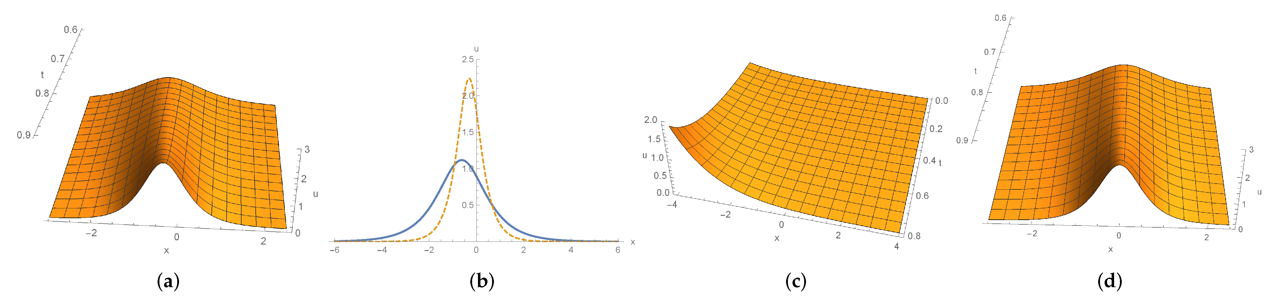
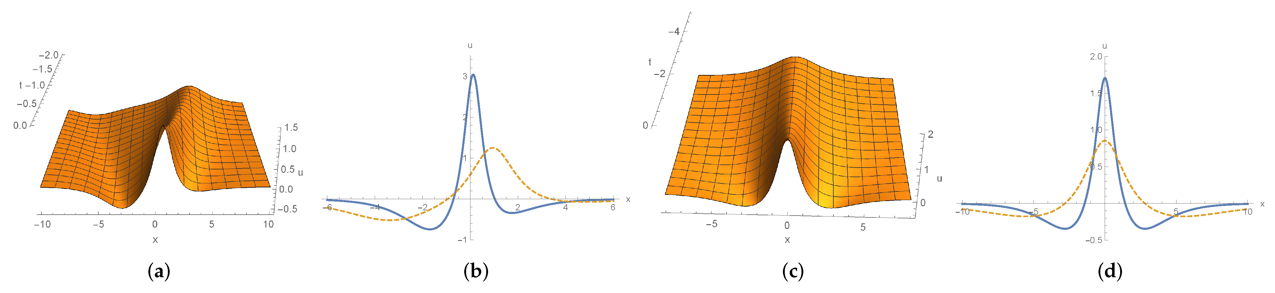
To present the explicit solutions of the local and nonlocal nmKdV-I Equation (27), we need to solve the matrix Equation (31). The first equation in (31) is the famous Sylvester Equation [44], which appears frequently in many areas of applied mathematics. To derive its solutions, we take $\Lambda \left(t\right)$ and T as the block matrices

$$\begin{array}{c}\hfill \Lambda \left(t\right)=\left(\begin{array}{cc}{\Lambda }_1\left(t\right)& \mathbf{0}\\ \mathbf{0}& {\Lambda }_2\left(t\right)\end{array}\right),T=\left(\begin{array}{cc}{T}_1& T_2\\ T_3& T_4\end{array}\right),\end{array}$$

(38)

with ${\Lambda }_i\left(t\right),T_j\in {\mathbb{C}}^{(n+1)\times (n+1)},i=1,2;j=1,2,3,4$. Substituting (38) into Equation (31) and noting that ${\Lambda }_{i,t}\left(t\right)={\Lambda }_i^3\left(t\right),(i=1,2)$, one can directly get the solutions for $\Lambda \left(t\right)$ and T. We list the solutions to (31) with different $(\sigma ,\delta )$ in

Table 1. $\Lambda \left(t\right)$ and T for Equation (31).

$(\mathit{\sigma },\mathit{\delta })$	$\mathbf{\Lambda }\left(\mathit{t}\right)$	T
(1, −1)	(38) with ${\Lambda }_2\left(t\right)=-{\Lambda }_1\left(t\right)$	$T_1=T_4=\mathbf{0},T_3=T_2=I$
(1, 1)	(38) with ${\Lambda }_2\left(t\right)=-{\Lambda }_1\left(t\right)$	$T_1=T_4=\mathbf{0},T_3=-T_2=I$
(−1, −1)	(38)	$T_1=-T_4=I,T_3=T_2=\mathbf{0}$
(−1, 1)	(38)	$T_1=-T_4=iI,T_3=T_2=\mathbf{0}$

.

In the following, we consider two types of solutions for the local and nonlocal nmKdV-I Equation (27), which are soliton solutions and Jordan block solutions. For the sake of brevity, we introduce some notations

$$\begin{array}{c}\hfill p_i={(a_i-2t)}^{-\frac{1}{2}},q_i={(b_i-2t)}^{-\frac{1}{2}},{\theta }_i=\frac{{\tilde{\alpha }}_i}{{\alpha }_i},(i=1,2,\dots ,n+1),\end{array}$$

(39)

where $\{{\tilde{\alpha }}_i={\alpha }_{n+1+i}\}$ and $\{a_i,b_i\}$ are complex constants.

Soliton solutions: Let ${\Lambda }_1\left(t\right)$ be the diagonal matrix, that is,

$$\begin{array}{c}\hfill {\Lambda }_1\left(t\right)=\mathrm{Diag}(p_1,p_2,\dots ,p_{n+1}).\end{array}$$

(40)

Remark 1.

In the case of $(\sigma ,\delta )=(-1,\pm 1)$, there is no restriction between ${\Lambda }_1\left(t\right)$ and ${\Lambda }_2\left(t\right)$. We can take ${\Lambda }_2\left(t\right)$ as

$$\begin{array}{c}\hfill {\Lambda }_2\left(t\right)=Diag(q_1,q_2,\dots ,q_{n+1}).\end{array}$$

(41)

Remark 2.

Because of the block structure of matrix T, one can easily observe that α can be gauged to be ${(1,1,\dots ,1;1,1,\cdots ,1)}^T$. This means the solutions obtained for the case $(\sigma =-1,\delta =\pm 1)$ are independent of phase parameters in α, that is, the initial phase has always to be zero. Soliton solutions and Jordan block solution listed below can demonstrate this character.

When $n=0$, we get the 1-soliton solutions

$$\begin{array}{cc}\hfill & u_{\sigma =1,\delta =-1}=p_{1}sech(p_{1}x+ln{\theta }_1),\hfill \end{array}$$

(42a)

$$\begin{array}{cc}\hfill & u_{\sigma =1,\delta =1}=p_{1}csch(p_{1}x+ln{\theta }_1),\hfill \end{array}$$

(42b)

$$\begin{array}{cc}\hfill & u_{\sigma =-1,\delta =-1}=\frac{p_1-q_1}{e^{p_{1}x}+e^{q_{1}x}},\hfill \end{array}$$

(42c)

$$\begin{array}{cc}\hfill & u_{\sigma =-1,\delta =1}=i\frac{p_1-q_1}{e^{p_{1}x}+e^{q_{1}x}}.\hfill \end{array}$$

(42d)

If we impose ${\Lambda }_2\left(t\right)=-{\Lambda }_1\left(t\right)$ into cases $(\sigma ,\delta )=(-1,\pm 1)$, we can get other 1-soliton solutions for these two cases

$$\begin{array}{cc}\hfill & u_{\sigma =-1,\delta =-1}=p_{1}sech\left(p_{1}x\right),\hfill \end{array}$$

(43a)

$$\begin{array}{cc}\hfill & u_{\sigma =-1,\delta =1}=i{p}_{1}sech\left(p_{1}x\right).\hfill \end{array}$$

(43b)

When $n=1$, one can get the 2-soliton solutions. For convenience, here we just write down the 2-soliton solutions with ${\Lambda }_2\left(t\right)=-{\Lambda }_1\left(t\right)$. They read

$$\begin{array}{cc}\hfill & u_{\sigma =1,\delta =-1}=\frac{4{\theta }_1{\theta }_2(p_1^2-p_2^2)e^{(p_1+p_2)x}(p_{1}cosh(p_{2}x+ln{\theta }_2)-p_{2}cosh(p_{1}x+ln{\theta }_1))}{2p_1{p}_2({({\theta }_1{e}^{p_{1}x}-{\theta }_2{e}^{p_{2}x})}^2-{(1+{\theta }_1{\theta }_2{e}^{(p_1+p_2)x})}^2)+\overline{c}\left(t\right)},\hfill \end{array}$$

(44a)

$$\begin{array}{cc}\hfill & u_{\sigma =1,\delta =1}=\frac{4{\theta }_1{\theta }_2(p_1^2-p_2^2)e^{(p_1+p_2)x}(p_{2}sinh(p_{1}x+ln{\theta }_1)-p_{1}sinh(p_{2}x+ln{\theta }_2))}{2p_1{p}_2({({\theta }_1{e}^{p_{1}x}-{\theta }_2{e}^{p_{2}x})}^2+{({\theta }_1{\theta }_2{e}^{(p_1+p_2)x}-1)}^2)+\overline{d}\left(t\right)},\hfill \end{array}$$

(44b)

$$\begin{array}{cc}\hfill & u_{\sigma =-1,\delta =-1}=\frac{(p_1^2-p_2^2)(p_{1}cosh\left(p_{2}x\right)-p_{2}cosh\left(p_{1}x\right))}{(p_1^2+p_2^2)cosh\left(p_{1}x\right)cosh\left(p_{2}x\right)-2p_1{p}_2(1+sinh\left(p_{1}x\right)sinh\left(p_{2}x\right))},\hfill \end{array}$$

(44c)

$$\begin{array}{cc}\hfill & u_{\sigma =-1,\delta =1}=\frac{i(p_1^2-p_2^2)(p_{1}cosh\left(p_{2}x\right)-p_{2}cosh\left(p_{1}x\right))}{(p_1^2+p_2^2)cosh\left(p_{1}x\right)cosh\left(p_{2}x\right)-2p_1{p}_2(1+sinh\left(p_{1}x\right)sinh\left(p_{2}x\right))},\hfill \end{array}$$

(44d)

in which

$$\begin{array}{cc}\hfill & \overline{c}\left(t\right)=(p_1^2+p_2^2)(1+{\theta }_1^2{e}^{2p_{1}x})(1+{\theta }_2^2{e}^{2p_{2}x}),\hfill \end{array}$$

(45a)

$$\begin{array}{cc}\hfill & \overline{d}\left(t\right)=(p_1^2+p_2^2)({\theta }_1^2{e}^{2p_{1}x}-1)(1-{\theta }_2^2{e}^{2p_{2}x}).\hfill \end{array}$$

(45b)

Jordan block solutions: To present elements of the basic Wronskian column vector of this case, we first introduce lower triangular Toeplitz (LTT) matrices which are defined as

$$\begin{array}{c}\hfill \mathcal{A}={\left(\begin{array}{cccccc}{\gamma }_0& 0& 0& \cdots & 0& 0\\ {\gamma }_1& {\gamma }_0& 0& \cdots & 0& 0\\ {\gamma }_2& {\gamma }_1& {\gamma }_0& \cdots & 0& 0\\ ⋮& ⋮& \cdots & ⋮& ⋮& ⋮\\ {\gamma }_{N-1}& {\gamma }_{N-2}& {\gamma }_{N-3}& \cdots & {\gamma }_1& {\gamma }_0\end{array}\right)}_{N\times N},{\gamma }_j\in \mathbb{C}.\end{array}$$

Note that all the LTT matrices of same order compose a commutative set in terms of matrix product. Canonical form of such a matrix is a Jordan matrix. LTT matrices play an important role in generating Jordan block (or multiple-pole or limit) solutions (cf. References [45,46]).

We take

$$\begin{array}{c}\hfill {\Lambda }_1\left(t\right)={\left({\lambda }_{s,j}\right)}_{(n+1)\times (n+1)},{\lambda }_{s,j}=\{\begin{array}{cc}\frac{1}{(s-j)!}{\partial }_{a_1}^{s-j}\frac{1}{2}{p}_1,\hfill & s\ge j,\hfill \\ 0,\hfill & s<j.\hfill \end{array}\end{array}$$

(46)

Similar to the discussion of soliton solutions, in this case $\varphi$ has two expressions with components

$$\begin{array}{c}\hfill {\varphi }_j=\{\begin{array}{cc}\frac{{\partial }_{a_1}^{j-1}}{(j-1)!}{\alpha }_1{(-\frac{\sqrt{2}}{2}{p}_1)}^{\frac{3}{2}-n}{e}^{\frac{p_{1}x}{2}},\hfill & j=1,2,\cdots ,n+1,\hfill \\ \frac{{\partial }_{b_1}^{s-1}}{(s-1)!}{\tilde{\alpha }}_1{(-\frac{\sqrt{2}}{2}{q}_1)}^{\frac{3}{2}-n}{e}^{\frac{q_{1}x}{2}},\hfill & j=n+1+s;s=1,2,\cdots ,n+1,\hfill \end{array}\end{array}$$

(47a)

or

$$\begin{array}{c}\hfill {\varphi }_j=\{\begin{array}{cc}\frac{{\partial }_{a_1}^{j-1}}{(j-1)!}{\alpha }_1{(-\frac{\sqrt{2}}{2}{p}_1)}^{\frac{3}{2}-n}{e}^{\frac{p_{1}x}{2}},\hfill & j=1,2,\cdots ,n+1,\hfill \\ \frac{{\partial }_{a_1}^{s-1}}{(s-1)!}{\tilde{\alpha }}_1{\left(\frac{\sqrt{2}}{2}{p}_1\right)}^{\frac{3}{2}-n}{e}^{-\frac{p_{1}x}{2}},\hfill & j=n+1+s;s=1,2,\cdots ,n+1.\hfill \end{array}\end{array}$$

(47b)

When $n=1$, we only list the solutions in the case of $(\sigma =1,\delta =-1)$ and $(\sigma =-1,\delta =-1)$, which are

$$\begin{array}{c}{u}_{\sigma =1,\delta =-1}=\frac{4p_1(cosh(p_{1}x-ln{\theta }_1)-p_{1}xsinh(p_{1}x-ln{\theta }_1))}{1+2{\left(p_{1}x\right)}^2+cosh\left(2(p_{1}x-ln{\theta }_1)\right)},\hfill \end{array}$$

(48a)

$$\begin{array}{c}{u}_{\sigma =-1,\delta =-1}=\frac{2(p_1-q_1)e^{\frac{(p_1+q_1)x}{2}}(2cosh\frac{(p_1-q_1)x}{2}-(p_1-q_1)xsinh\frac{(p_1-q_1)x}{2})}{2+{\left((p_1-q_1)x\right)}^2+2cosh\frac{(p_1-q_1)x}{2}},\hfill \end{array}$$

(48b)

$$\begin{array}{c}{u}_{\sigma =-1,\delta =-1}=\frac{4p_1(cosh\left(p_{1}x\right)-p_{1}xsinh\left(p_{1}x\right))}{1+2{\left(p_{1}x\right)}^2+cosh\left(2p_{1}x\right)}.\hfill \end{array}$$

(48c)

3.2.3. Dynamics

Now let us consider the dynamics of the obtained 1-soliton solution, 2-soliton solutions and Jordan block solutions, where we need to take $t<min\{\frac{a_j}{2},\frac{b_j}{2}\}$ in order to guarantee the real properties of components $p_i$ and $q_i$. It is obvious that $p_i>0$ and $q_i>0$ for $i=1,2$. With no loss of generality we just consider the dynamics of $u_{\sigma =1,\delta =-1}$ and $u_{\sigma =-1,\delta =-1}$. We first identify the dynamics of 1-soliton solution given by (42a), (42c) and (43a). Solution (42a) is nonsingular soliton wave with initial phase $ln{\theta }_1$. Moreover, the part $p_1$ defines a time varying amplitude due to the nonisospectral effect. The top trace is given by the point trace

$$\begin{array}{c}\hfill x\left(t\right)=-p_1^{-1}ln{\theta }_1.\end{array}$$

(49)

Furthermore,

$$\begin{array}{c}\hfill \frac{dx\left(t\right)}{dt}=-p_{1}ln{\theta }_1\end{array}$$

(50)

implies the time-varying velocity of the wave. For the solution (42c), it is easy to find that for fixed t, $u_{\sigma =-1,\delta =-1}\to 0$ as $x\to +\infty$ and $u_{\sigma =-1,\delta =-1}\to \infty$ as $x\to -\infty$. For the solution (43a), one can find that it is exactly the solution (42a) with ${\theta }_1=1$, which appears as a stationary soliton with top trace $x=0$. We illustrate these three solitons in Figure 1.

We next to pay attention to the 2-soliton solutions (44). Since $p_1$ and $p_2$ are functions of t, it is intractable to make asymptotic analysis as usual [47]. Here, we only depict (44a) and (44c) in Figure 2. We illustrate the Jordan block solutions (48) in Figure 3.

As shown in Figure 2, for fixed t, solution (44c) is an even function of x and also appears as stationary solitons. For the Jordan block solution (48c), one can notice that it is a stationary wave and is symmetric with respect to x.

3.3. Complex Local and Nonlocal Reductions

In this subsection, we mainly realize the complex local and nonlocal reductions of the nAKNS(3) Equation (3). We impose complex reduction

$$\begin{array}{c}\hfill v\left(x\right)=\delta u^{*}\left(\sigma x\right),\sigma =\pm 1,\end{array}$$

(51)

into (3) and then catch the complex equation

$$\begin{array}{cc}\hfill u_t=& x(u_{xxx}-6\delta u{u}^{*}\left(\sigma x\right)u_x)+3(u_{xx}-2\delta u^2{u}^{*}\left(\sigma x\right))\hfill \\ & -2\delta u_x{\partial }^{-1}u{u}^{*}\left(\sigma x\right)+4\delta u{\partial }^{-1}u{u}_x^{*}\left(\sigma x\right),\hfill \end{array}$$

(52)

which is the local nmKdV-II Equation (6) when $\sigma =1$ and the nonlocal nmKdV-II equation when $\sigma =-1$. Equation (52) is preserved under transformations $u\to -u$ and $u\to \pm iu$. Since the discussion is similar to the real reduction, here we skip the proof and only present the related constraint conditions and solutions of Equation (52) in the following theorem.

Theorem 3.

Exact solutions of the local and nonlocal nmKdV-II Equation (52) are given by

$$\begin{array}{c}\hfill u=\frac{g}{f},f=|{\widehat{\varphi }}^{\left(n\right)};{\widehat{\psi }}^{\left(n\right)}|,g=2|{\widehat{\varphi }}^{(n+1)};{\widehat{\psi }}^{(n-1)}|,\end{array}$$

(53)

in which ϕ and ψ are the $2(n+1)$th order column vectors defined by (25), and satisfy the following relation

$$\begin{array}{c}\hfill \psi \left(x\right)={(-\sigma )}^{\frac{3}{2}-n}T{\varphi }^{*}\left(\sigma x\right),\end{array}$$

(54)

where $T\in {\mathbb{C}}^{2(n+1)\times 2(n+1)}$ in (54) is a constant matrix satisfying

$$\begin{array}{c}\hfill \Lambda \left(t\right)T+\sigma T{\Lambda }^{*}\left(t\right)=0,T{T}^{*}=-\delta I,\end{array}$$

(55)

and we require $\beta =T{\alpha }^{*}$.

We skip the proof here, which is similar to the one for Theorem 2. Based on the Theorem 3 we know that $u=\frac{g}{f}$ together with

$$\begin{array}{c}\hfill f=|{\widehat{\varphi }}^{\left(n\right)}\left(x\right);{(-\sigma )}^{\frac{3}{2}-n}T{\widehat{\varphi }}^{{\left(n\right)}^{*}}\left(\sigma x\right)|,g=2|{\widehat{\varphi }}^{(n+1)}\left(x\right);{(-\sigma )}^{\frac{3}{2}-n}T{\widehat{\varphi }}^{{(n-1)}^{*}}\left(\sigma x\right)|,\end{array}$$

(56)

solves the local and nonlocal nmKdV-II Equation (52), where $\varphi$ is given by (25) and $\Lambda \left(t\right)$ and T satisfy the constraint relations (55).

In order to solve the constraint Equations (55), we still decompose matrices $\Lambda \left(t\right)$ and T as (38). We list the solutions to (55) in

Table 2. $\Lambda \left(t\right)$ and T for Equation (55).

$(\mathit{\sigma },\mathit{\delta })$	$\mathbf{\Lambda }\left(\mathit{t}\right)$	T
(1, −1)	(38) with ${\Lambda }_2\left(t\right)=-{\Lambda }_1^{*}\left(t\right)$	$T_1=T_4=\mathbf{0},T_3=T_2=I$
(1, 1)	(38) with ${\Lambda }_2\left(t\right)=-{\Lambda }_1^{*}\left(t\right)$	$T_1=T_4=\mathbf{0},T_3=-T_2=I$
(−1, −1)	(38) with ${\Lambda }_2\left(t\right)={\Lambda }_1^{*}\left(t\right)$	$T_1=T_4=\mathbf{0},T_3=T_2=I$
(−1, 1)	(38) with ${\Lambda }_2\left(t\right)={\Lambda }_1^{*}\left(t\right)$	$T_1=T_4=\mathbf{0},T_3=-T_2=I$

.

Since the involvement of complex conjugate, here we just consider the soliton solutions for the local and nonlocal nmKdV-II Equation (52). For convenience, we denote

$$\begin{array}{c}\hfill k_j={(c_j-2t)}^{-\frac{1}{2}},(j=1,2,\dots ,n+1),\end{array}$$

(57)

where $c_j=c_{j1}+i{c}_{j2},(j=1,2,\dots ,n+1)$ are complex constants. Soliton solutions can be derived by taking

$$\begin{array}{c}\hfill {\Lambda }_1\left(t\right)=\mathrm{Diag}(k_1,k_2,\dots ,k_{n+1}).\end{array}$$

(58)

In particular, with different $(\sigma ,\delta )$, the 1-soliton solution of Equation (52) can be described as

$$\begin{array}{c}{u}_{\sigma =1,\delta =-1}=\frac{{\alpha }_1{\tilde{\alpha }}_1(k_1+k_1^{*})}{|{\alpha }_1{|}^2{e}^{-x{k}_1^{*}}+{\left|{\tilde{\alpha }}_1\right|}^2{e}^{x{k}_1}},\hfill \end{array}$$

(59a)

$$\begin{array}{c}{u}_{\sigma =1,\delta =1}=\frac{{\alpha }_1{\tilde{\alpha }}_1(k_1+k_1^{*})}{|{\alpha }_1{|}^2{e}^{-x{k}_1^{*}}-{\left|{\tilde{\alpha }}_1\right|}^2{e}^{x{k}_1}},\hfill \end{array}$$

(59b)

$$\begin{array}{c}{u}_{\sigma =-1,\delta =-1}=\frac{{\alpha }_1{\tilde{\alpha }}_1(k_1-k_1^{*})}{|{\alpha }_1{|}^2{e}^{x{k}_1^{*}}-{\left|{\tilde{\alpha }}_1\right|}^2{e}^{x{k}_1}},\hfill \end{array}$$

(59c)

$$\begin{array}{c}{u}_{\sigma =-1,\delta =1}=\frac{{\alpha }_1{\tilde{\alpha }}_1(k_1-k_1^{*})}{|{\alpha }_1{|}^2{e}^{x{k}_1^{*}}+{\left|{\tilde{\alpha }}_1\right|}^2{e}^{x{k}_1}},\hfill \end{array}$$

(59d)

where $|·|$ means module.

Now let us consider the dynamics of solutions (59). We denote $k_1$ as $k_1={(\mu +i\nu )}^{-1}$ and substitute it back into (57) with $j=1$. Equating the real part and imaginary part, the result is

$$\begin{array}{c}\hfill \mu =\frac{c_{12}}{2\nu },\nu =\frac{1}{\sqrt{2}}{\left(2t-c_{11}+\sqrt{{(c_{11}-2t)}^2+c_{12}^2}\right)}^{\frac{1}{2}}.\end{array}$$

(60)

Taking $k_1={(\mu +i\nu )}^{-1}$ into (59), we rewrite it as

$$\begin{array}{c}{u}_{\sigma =1,\delta =-1}=\frac{2{\alpha }_1{\tilde{\alpha }}_1\mu }{({\mu }^2+{\nu }^2)\left(\right|{\alpha }_1{|}^2{e}^{-\frac{x}{\mu -i\nu }}+|{\tilde{\alpha }}_1{|}^2{e}^{\frac{x}{\mu +i\nu }})},\hfill \end{array}$$

(61a)

$$\begin{array}{c}{u}_{\sigma =1,\delta =1}=\frac{2{\alpha }_1{\tilde{\alpha }}_1\mu }{({\mu }^2+{\nu }^2)\left(\right|{\alpha }_1{|}^2{e}^{-\frac{x}{\mu -i\nu }}-|{\tilde{\alpha }}_1{|}^2{e}^{\frac{x}{\mu +i\nu }})},\hfill \end{array}$$

(61b)

$$\begin{array}{c}{u}_{\sigma =-1,\delta =-1}=\frac{-2i{\alpha }_1{\tilde{\alpha }}_1\nu }{({\mu }^2+{\nu }^2)\left(\right|{\alpha }_1{|}^2{e}^{\frac{x}{\mu -i\nu }}-|{\tilde{\alpha }}_1{|}^2{e}^{\frac{x}{\mu +i\nu }})},\hfill \end{array}$$

(61c)

$$\begin{array}{c}{u}_{\sigma =-1,\delta =1}=\frac{-2i{\alpha }_1{\tilde{\alpha }}_1\nu }{({\mu }^2+{\nu }^2)\left(\right|{\alpha }_1{|}^2{e}^{\frac{x}{\mu -i\nu }}+|{\tilde{\alpha }}_1{|}^2{e}^{\frac{x}{\mu +i\nu }})}.\hfill \end{array}$$

(61d)

To proceed, we present an analysis of the dynamics of ${\left|u\right|}_{\sigma =1,\delta =-1}^2$ and ${\left|u\right|}_{\sigma =-1,\delta =-1}^2$. For the solution (61a), we know that

$$\begin{array}{c}\hfill {\left|u\right|}_{\sigma =1,\delta =-1}^2=\frac{{\mu }^2}{{({\mu }^2+{\nu }^2)}^2}{sech}^2\left(\frac{\mu x}{{\mu }^2+{\nu }^2}+ln\left|\frac{{\tilde{\alpha }}_1}{{\alpha }_1}\right|\right).\end{array}$$

(62)

The part $\frac{{\mu }^2}{{({\mu }^2+{\nu }^2)}^2}$ implies a time varying amplitude, which tends to zero as $t\to \pm \infty$. Besides, the part ${sech}^2\left(\frac{\mu x}{{\mu }^2+{\nu }^2}+ln\left|\frac{{\tilde{\alpha }}_1}{{\alpha }_1}\right|\right)$ is Gaussian-distributed with respect to x for a given t. Figure 4 shows that the central amplitude is higher than both the background and the amplitude of this soliton. Thus we view central peak as a rogue wave. The top trace of (62) is

$$\begin{array}{c}\hfill x=\frac{{\mu }^2+{\nu }^2}{\mu }ln\left|\frac{{\alpha }_1}{{\tilde{\alpha }}_1}\right|,\end{array}$$

(63)

and the traveling speed is

$$\begin{array}{c}\hfill x^{\prime }\left(t\right)=\frac{2\nu (2{\nu }^2+2t-c_{11})}{c_{12}(2{\nu }^2-2t+c_{11})}ln\left|\frac{{\alpha }_1}{{\tilde{\alpha }}_1}\right|.\end{array}$$

(64)

When $|{\alpha }_1|=|{\tilde{\alpha }}_1|$, (62) exhibits a stationary rogue wave with top trace $x=0$.

For solution (61c) we observe that

$$\begin{array}{c}\hfill {\left|u\right|}_{\sigma =-1,\delta =-1}^2=\frac{4|{\alpha }_1{\tilde{\alpha }}_1{\nu |}^2{e}^{-\frac{2x\mu }{{\mu }^2+{\nu }^2}}}{{({\mu }^2+{\nu }^2)}^2\left(\right|{\alpha }_1{|}^4+|{\tilde{\alpha }}_1{|}^4-2|{\alpha }_1{\tilde{\alpha }}_1{|}^{2}cos\frac{2x\nu }{{\mu }^2+{\nu }^2})}.\end{array}$$

(65)

When $|{\alpha }_1|=|{\tilde{\alpha }}_1|$, ${\left|u\right|}_{\sigma =-1,\delta =-1}^2$ has singularities along

$$\begin{array}{c}\hfill x\left(t\right)=\frac{\kappa \pi ({\mu }^2+{\nu }^2)}{\nu },\kappa \in \mathbb{Z}.\end{array}$$

(66)

While when $|{\alpha }_1|\ne |{\tilde{\alpha }}_1|$, ${\left|u\right|}_{\sigma =-1,\delta =-1}^2$ is a nonsingular wave. For fixed t, it tends to zero as $x\to +\infty$ and tends to $+\infty$ as $x\to -\infty$. Because of the involvement of cosine function in denominator, there is quasi-periodic phenomenon. We depict this solution in Figure 5.

4. Local and Nonlocal Reductions of the nAKNS(-1) Equation (4)

In this section, we shall use a similar strategy to consider the local and nonlocal reductions of the nAKNS(-1) Equation (4). Real nonlocal reduction and complex nonlocal reduction will be applied to the nAKNS(-1) Equation (4). Consequently, a nonlocal nsG-I equation (real form) and a nonlocal nsG-II equation (complex form) will be presented. Soliton solutions and Jordan block solutions for the local and nonlocal nsG-I equations and local and nonlocal nsG-II equations will be discussed. Dynamics will also be studied.

4.1. Double Wronskian Solutions

Before considering the local and nonlocal reductions we reveal the bilinearization and double Wronskian solutions for the nAKNS(-1) Equation (4).

Through the dependent variable transformations

$$\begin{array}{c}\hfill u=\frac{g}{f},v=\frac{h}{f},\end{array}$$

(67)

the nAKNS(-1) Equation (4) is transformed into the bilinear form

$$\begin{array}{c}{D}_x{D}_{t}g·f-xgf=0,\hfill \end{array}$$

(68a)

$$\begin{array}{c}{D}_x{D}_{t}h·f-xhf=0,\hfill \end{array}$$

(68b)

$$\begin{array}{c}{D}_x^{2}f·f-2gh=0.\hfill \end{array}$$

(68c)

Double Wronski determinant solutions of bilinear form (68) are presented by the following theorem.

Theorem 4.

The double Wronski determinants

$$\begin{array}{c}\hfill f=|{\widehat{\varphi }}^{\left(n\right)};{\widehat{\psi }}^{\left(m\right)}|,g=2|{\widehat{\varphi }}^{(n+1)};{\widehat{\psi }}^{(m-1)}|,h=2|{\widehat{\varphi }}^{(n-1)};{\widehat{\psi }}^{(m+1)}|,\end{array}$$

(69)

solve the bilinear system (68), provided that ϕ and ψ satisfy the following condition equation set

$$\begin{array}{cc}\hfill & {\varphi }_x=-\frac{\Omega \left(t\right)}{2}\varphi ,{\psi }_x=\frac{\Omega \left(t\right)}{2}\psi ,\hfill \end{array}$$

(70a)

$$\begin{array}{cc}\hfill & {\varphi }_t=\frac{x}{4}{\partial }^{-1}\varphi -\frac{1}{4}{\partial }^{-2}\varphi ,{\psi }_t=\frac{x}{4}{\partial }^{-1}\psi -\frac{1}{4}{\partial }^{-2}\psi ,\hfill \end{array}$$

(70b)

respectively, where $\Omega \left(t\right)$ is an $(n+m+2)\times (n+m+2)$ matrix satisfying ${\Omega }_t\left(t\right)={\Omega }^{-1}\left(t\right)$.

Solving the condition equation set (70), we know that the column vectors $\varphi$ and $\psi$ are given by

$$\begin{array}{c}\varphi ={\Omega }^{-1}\left(t\right)e^{-\frac{\Omega \left(t\right)}{2}x}\alpha ,\psi ={\Omega }^{-1}\left(t\right)e^{\frac{\Omega \left(t\right)}{2}x}\beta ,\hfill \end{array}$$

(71)

where $\alpha$ and $\beta$ are two constant column vectors given by (25b).

In the following two subsections, we consider the real local and nonlocal reductions and the complex local and nonlocal reductions of the nAKNS(-1) Equation (4), respectively. We take $m=n$ and follow the ideas of Section 3.1 and Section 3.2. We will see that the nonlocal nsG-I equation and the nonlocal nsG-II equation are also reverse space type.

4.2. Real Local and Nonlocal Reductions

Applying constraint

$$\begin{array}{c}\hfill v\left(x\right)=\delta u\left(\sigma x\right)\sigma =\pm 1,\end{array}$$

(72)

to the nAKNS(-1) Equation (4), we reach to equation

$$\begin{array}{c}\hfill u_{xt}+2\delta u{\partial }^{-1}{\left(uu\left(\sigma x\right)\right)}_t=xu,\end{array}$$

(73)

which is the local nsG-I Equation (7) when $\sigma =1$ and the nonlocal nsG-I Equation when $\sigma =-1$. It is easy to understand that Equation (73) is preserved under transformation $u\to -u$. Meanwhile, Equation (73) with $(\sigma ,\delta )=(\pm 1,1)$ and with $(\sigma ,\delta )=(\pm 1,-1)$ can be transformed from each other by taking $u\to \pm iu$.

Remark 3.

Similar to the isospectral case (cf. Reference [34]), we view the Equation (7) with $\delta =1$ as a nonpotential form of the nonisospectral sG equation

$$\begin{array}{c}\hfill w_{tx}=xsinw-cosw{\partial }^{-1}sinw+sinw{\partial }^{-1}(cosw-1).\end{array}$$

(74)

In fact, we introduce an auxiliary function ρ satisfying ${\rho }_x={\left(u^2\right)}_t$, then (7) yields

$$\begin{array}{c}\hfill u_{xt}+2u\rho =xu,{\left(u^2\right)}_t={\rho }_x.\end{array}$$

(75)

Via the transformations (cf. Reference [48,49])

$$\begin{array}{c}\hfill u=\frac{w_x}{2},\rho =-\frac{1}{2}((x+cosw{\partial }^{-1})(cosw-1)+sinw{\partial }^{-1}sinw),\end{array}$$

(76)

system (75) can be transformed into

$$\begin{array}{cc}\hfill & u_{xt}+2u\rho -xu=\frac{1}{2}{[w_{xt}-(xsinw-cosw{\partial }^{-1}sinw+sinw{\partial }^{-1}(cosw-1))]}_x,\hfill \end{array}$$

(77a)

$$\begin{array}{cc}\hfill & {\left(u^2\right)}_t-{\rho }_x=\frac{w_x}{2}[w_{xt}-(xsinw-cosw{\partial }^{-1}sinw+sinw{\partial }^{-1}(cosw-1))].\hfill \end{array}$$

(77b)

Thus we call the Equation (7) with $\delta =1$ as a nonpotential nonisospectral sG equation.

Analogous to the previous analysis, double Wronski determinant solutions to local and nonlocal nsG-I Equation (73) can be summerized by the following theorem.

Theorem 5.

Exact solutions of the local and nonlocal nsG-I Equation (73) are given by

$$\begin{array}{c}\hfill u=\frac{g}{f},f=|{\widehat{\varphi }}^{\left(n\right)}\left(x\right);-\sigma T{\widehat{\varphi }}^{\left(n\right)}\left(\sigma x\right)|,g=2|{\widehat{\varphi }}^{(n+1)}\left(x\right);-\sigma T{\widehat{\varphi }}^{(n-1)}\left(\sigma x\right)|,\end{array}$$

(78)

in which ϕ is the $2(n+1)$th order column vector defined by (71) and $T\in {\mathbb{C}}^{2(n+1)\times 2(n+1)}$ is a constant matrix satisfying

$$\begin{array}{c}\hfill \Omega \left(t\right)T+\sigma T\Omega \left(t\right)=\mathbf{0},T^2=-\sigma \delta I.\end{array}$$

(79)

4.2.1. Some Examples of Solutions

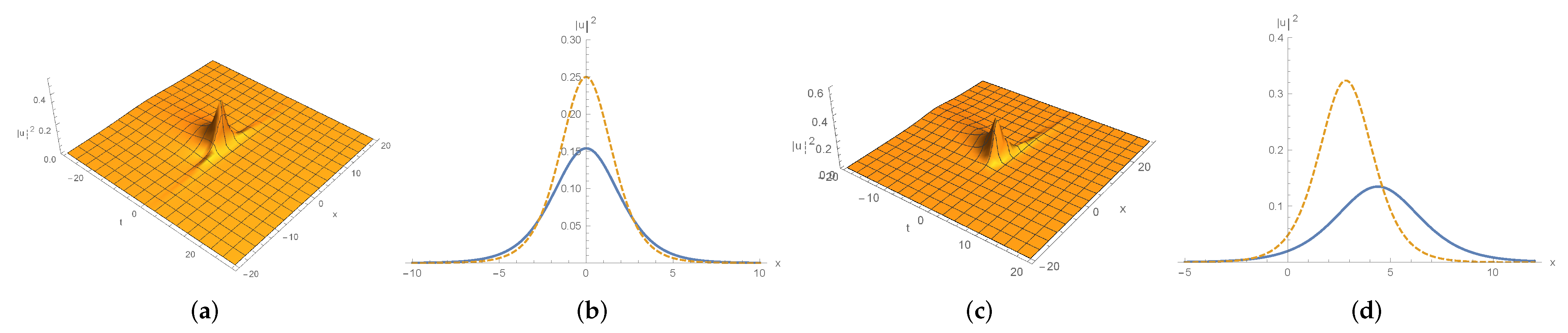
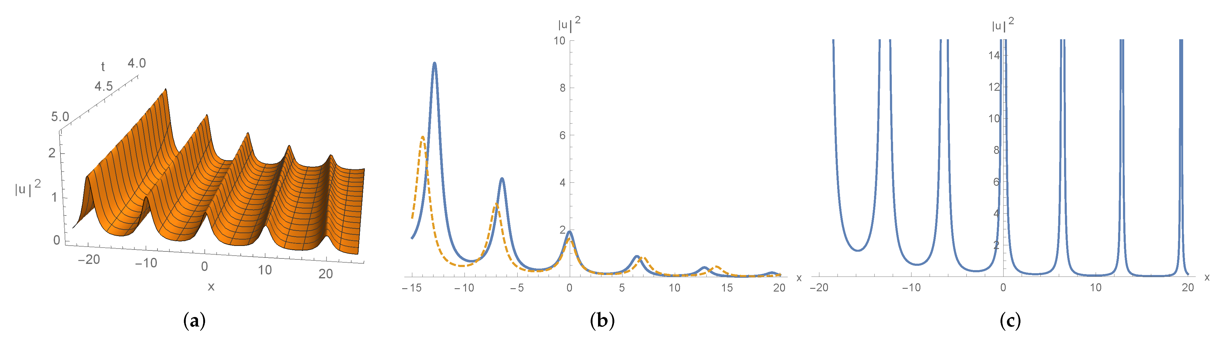
We shall now derive, starting from (79), solutions for the local and nonlocal nsG-I Equation (73). We take $\Omega \left(t\right)$ and T as the block matrices

$$\begin{array}{c}\hfill \Omega \left(t\right)=\left(\begin{array}{cc}{\Omega }_1\left(t\right)& \mathbf{0}\\ \mathbf{0}& {\Omega }_2\left(t\right)\end{array}\right),T=\left(\begin{array}{cc}{T}_1& T_2\\ T_3& T_4\end{array}\right),\end{array}$$

(80)

with ${\Omega }_i\left(t\right),T_j\in {\mathbb{C}}^{(n+1)\times (n+1)},i=1,2;j=1,2,3,4$. Substituting (80) into Equation (79) and performing straightforward calculation, one can realize the relations between ${\Omega }_1\left(t\right)$ and ${\Omega }_2\left(t\right)$. In addition, the form of T can be determined. We list the solutions to (79) with different $(\sigma ,\delta )$ in

Table 3. $\Omega \left(t\right)$ and T for Equation (79).

$(\mathit{\sigma },\mathit{\delta })$	$\mathbf{\Omega }\left(\mathit{t}\right)$	T
(1,1)	(80) with  ${\Omega }_2\left(t\right)=-{\Omega }_1\left(t\right)$	$T_1=T_4={\mathbf{0}}_{n+1},T_3=-T_2=I$
(1,−1)	(80) with  ${\Omega }_2\left(t\right)=-{\Omega }_1\left(t\right)$	$T_1=T_4={\mathbf{0}}_{n+1},T_3=T_2=I$
(−1,1)	(80)	$T_1=-T_4=I,T_3=T_2=\mathbf{0}$
(−1,−1)	(80)	$T_1=-T_4=iI,T_3=T_2=\mathbf{0}$

.

To proceed, we introduce two notations

$$\begin{array}{c}\hfill r_i={(2t+d_i)}^{\frac{1}{2}},s_i={(2t+e_i)}^{\frac{1}{2}},(i=1,2,\dots ,n+1),\end{array}$$

(81)

where $\{d_i,e_i\}$ are complex constants. We will now list soliton solutions and Jordan block solutions to the Equation (73) in terms of the different forms of ${\Omega }_1\left(t\right)$ and ${\Omega }_2\left(t\right)$.

Soliton solutions: Let ${\Omega }_1\left(t\right)$ be the diagonal matrix

$$\begin{array}{c}\hfill {\Omega }_1\left(t\right)=\mathrm{Diag}(r_1,r_2,\dots ,r_{n+1}).\end{array}$$

(82)

Then for cases $(\sigma ,\delta )=(1,\pm 1)$, one has to take

$$\begin{array}{c}\hfill {\Omega }_2\left(t\right)=\mathrm{Diag}(-r_1,-r_2,\dots ,-r_{n+1}).\end{array}$$

(83)

While for cases $(\sigma ,\delta )=(-1,\pm 1)$, ${\Omega }_2\left(t\right)$ can be taken as (83) or

$$\begin{array}{c}\hfill {\Omega }_2\left(t\right)=\mathrm{Diag}(s_1,s_2,\dots ,s_{n+1}).\end{array}$$

(84)

We can also observe that solutions in the cases $(\sigma =-1,\delta =\pm 1)$ are independent of phase parameters in $\alpha$, since it is gauged to be ${(1,1,\dots ,1;1,1,\cdots ,1)}^T$. The 1-soliton solutions read

$$\begin{array}{cc}\hfill & u_{\sigma =1,\delta =1}=r_{1}sech(r_{1}x+ln{\theta }_1),\hfill \end{array}$$

(85a)

$$\begin{array}{cc}\hfill & u_{\sigma =1,\delta =-1}=r_{1}csch(r_{1}x+ln{\theta }_1),\hfill \end{array}$$

(85b)

$$\begin{array}{cc}\hfill & u_{\sigma =-1,\delta =1}=r_{1}sech\left(r_{1}x\right),\mathrm{with}{\Omega }_2\mathrm{given}\mathrm{by}\left(83\right),\hfill \end{array}$$

(85c)

$$\begin{array}{cc}\hfill & u_{\sigma =-1,\delta =-1}=i{r}_{1}sech\left(r_{1}x\right),\mathrm{with}{\Omega }_2\mathrm{given}\mathrm{by}\left(83\right),\hfill \end{array}$$

(85d)

$$\begin{array}{cc}\hfill & u_{\sigma =-1,\delta =1}=\frac{(r_1-s_1)}{e^{r_{1}x}+e^{s_{1}x}},\mathrm{with}{\Omega }_2\mathrm{given}\mathrm{by}\left(84\right),\hfill \end{array}$$

(85e)

$$\begin{array}{cc}\hfill & u_{\sigma =-1,\delta =-1}=i\frac{(r_1-s_1)}{e^{r_{1}x}+e^{s_{1}x}},\mathrm{with}{\Omega }_2\mathrm{given}\mathrm{by}\left(84\right),\hfill \end{array}$$

(85f)

where ${\theta }_1$ is defined by (39).

When $n=1$, we list the 2-soliton solutions with ${\Omega }_2\left(t\right)=-{\Omega }_1\left(t\right)$, which are

$$\begin{array}{cc}\hfill & u_{\sigma =1,\delta =1}=\frac{4{\theta }_1{\theta }_2(r_1^2-r_2^2)e^{(r_1+r_2)x}(r_{1}cosh(r_{2}x+ln{\theta }_2)-r_{2}cosh(r_{1}x+ln{\theta }_1))}{2r_1{r}_2({({\theta }_1{e}^{r_{1}x}-{\theta }_2{e}^{r_{2}x})}^2-{(1+{\theta }_1{\theta }_2{e}^{(r_1+r_2)})}^2)+\overline{a}\left(t\right)},\hfill \end{array}$$

(86a)

$$\begin{array}{cc}\hfill & u_{\sigma =1,\delta =-1}=\frac{4{\theta }_1{\theta }_2(r_1^2-r_2^2)e^{(r_1+r_2)x}(r_{2}sinh(r_{1}x+ln{\theta }_1)-r_{1}sinh(r_{2}x+ln{\theta }_2))}{2r_1{r}_2({({\theta }_1{e}^{r_{1}x}-{\theta }_2{e}^{r_{2}x})}^2+{({\theta }_1{\theta }_2{e}^{(r_1+r_2)}-1)}^2)+\overline{b}\left(t\right)},\hfill \end{array}$$

(86b)

$$\begin{array}{cc}\hfill & u_{\sigma =-1,\delta =1}=\frac{(r_1^2-r_2^2)(r_{1}cosh\left(r_{2}x\right)-r_{2}cosh\left(r_{1}x\right))}{(r_1^2+r_2^2)cosh\left(r_{1}x\right)cosh\left(r_{2}x\right)-2r_1{r}_2(1+sinh\left(r_{1}x\right)sinh\left(r_{2}x\right))},\hfill \end{array}$$

(86c)

$$\begin{array}{cc}\hfill & u_{\sigma =-1,\delta =-1}=\frac{i(r_1^2-r_2^2)(r_{1}cosh\left(r_{2}x\right)-r_{2}cosh\left(r_{1}x\right))}{(r_1^2+r_2^2)cosh\left(r_{1}x\right)cosh\left(r_{2}x\right)-2r_1{r}_2(1+sinh\left(r_{1}x\right)sinh\left(r_{2}x\right))},\hfill \end{array}$$

(86d)

where

$$\begin{array}{cc}\hfill & \overline{a}\left(t\right)=(r_1^2+r_2^2)(1+{\theta }_1^2{e}^{2r_{1}x})(1+{\theta }_2^2{e}^{2r_{2}x}),\hfill \end{array}$$

(87a)

$$\begin{array}{cc}\hfill & \overline{b}\left(t\right)=(r_1^2+r_2^2)({\theta }_1^2{e}^{2r_{1}x}-1)(1-{\theta }_2^2{e}^{2r_{2}x}).\hfill \end{array}$$

(87b)

Jordan block solutions: We take

$$\begin{array}{c}\hfill {\Omega }_1\left(t\right)={\left({\omega }_{s,j}\right)}_{(n+1)\times (n+1)},{\omega }_{s,j}=\{\begin{array}{cc}\frac{1}{(s-j)!}{\partial }_{d_1}^{s-j}\frac{1}{2}{r}_1,\hfill & s\ge j,\hfill \\ 0,\hfill & s<j.\hfill \end{array}\end{array}$$

(88)

Then with different ${\Omega }_2$, $\varphi$ has two expressions with components

$$\begin{array}{c}\hfill {\varphi }_j=\{\begin{array}{cc}\frac{{\partial }_{d_1}^{j-1}}{(j-1)!}{\alpha }_1{(-r_1)}^{-1}{e}^{\frac{r_{1}x}{2}},\hfill & j=1,2,\cdots ,n+1,\hfill \\ \frac{{\partial }_{d_1}^{s-1}}{(s-1)!}{\tilde{\alpha }}_1{\left(r_1\right)}^{-1}{e}^{-\frac{r_{1}x}{2}},\hfill & j=n+1+s;s=1,2,\cdots ,n+1,\hfill \end{array}\end{array}$$

(89a)

or

$$\begin{array}{c}\hfill {\varphi }_j=\{\begin{array}{cc}\frac{{\partial }_{d_1}^{j-1}}{(j-1)!}{\alpha }_1{(-r_1)}^{-1}{e}^{\frac{r_{1}x}{2}},\hfill & j=1,2,\cdots ,n+1,\hfill \\ \frac{{\partial }_{e_1}^{s-1}}{(s-1)!}{\tilde{\alpha }}_1{(-s_1)}^{-1}{e}^{\frac{s_{1}x}{2}},\hfill & j=n+1+s;s=1,2,\cdots ,n+1.\hfill \end{array}\end{array}$$

(89b)

When $n=1$, we give the solutions in the case of $(\sigma =1,\delta =1)$ and $(\sigma =-1,\delta =1)$, which are

$$\begin{array}{cc}\hfill & u_{\sigma =1,\delta =1}=\frac{4r_1(cosh(r_{1}x-ln{\theta }_1)-r_{1}xsinh(r_{1}x-ln{\theta }_1))}{1+2{\left(r_{1}x\right)}^2+cosh\left(2(r_{1}x-ln{\theta }_1)\right)},\hfill \end{array}$$

(90a)

$$\begin{array}{cc}\hfill & u_{\sigma =-1,\delta =1}=\frac{4r_1(cosh\left(r_{1}x\right)-r_{1}xsinh\left(r_{1}x\right))}{1+2{\left(r_{1}x\right)}^2+cosh\left(2r_{1}x\right)},\hfill \end{array}$$

(90b)

$$\begin{array}{cc}\hfill & u_{\sigma =-1,\delta =1}=\frac{2(r_1-s_1)e^{(r_1+s_1)x}((r_1-s_1)xsinh\left((r_1-s_1)x\right)-2cosh\left((r_1-s_1)x\right))}{2+(r_1^2-s_1^2)x^2+2cosh\left((r_1-s_1)x\right)}.\hfill \end{array}$$

(90c)

4.2.2. Dynamics

We now examine the dynamics of some obtained solutions, where we take $t<min\{-\frac{d_j}{2},-\frac{e_j}{2}\}$ in order to guarantee the real properties of components $r_i$ and $s_i$. Here we just consider the dynamics of $u_{\sigma =1,\delta =1}$ and $u_{\sigma =-1,\delta =1}$ without loss of generality. To proceed, we consider the 1-soliton solution (85a). This is a nonsingular soliton wave with initial phase $ln{\theta }_1$ and asymptotically follows:

$$\begin{array}{cc}\hfill \mathrm{amplitude}:& u=r_1,\hfill \end{array}$$

(91a)

$$\begin{array}{cc}\hfill \mathrm{top}\mathrm{point}\mathrm{traces}:& x\left(t\right)=-r_1^{-1}ln{\theta }_1,\hfill \end{array}$$

(91b)

$$\begin{array}{cc}\hfill \mathrm{speed}:& \frac{dx}{dt}=-r_{1}ln{\theta }_1.\hfill \end{array}$$

(91c)

To continue we next consider (85c) and (85e). The solution (85c) is symmetric with respect to x and describes a stationary wave. With regards to the solution (85e), for fixed t, it tends to zero as $x\to +\infty$ and tends to ∞ as $x\to -\infty$. We depict these solitons in Figure 6.

For the 2-soliton solutions (86) and Jordan block solutions (90), one can find that $u_{\sigma =-1,\delta =1}$ in (86c) and (90b) are even functions of x and describe stationary waves. We illustrate them in Figure 7 and Figure 8.

4.3. Complex Local and Nonlocal Reductions

Now let us consider the complex local and nonlocal reductions of the nAKNS(-1) Equation (4). By the constraint

$$\begin{array}{c}\hfill v\left(x\right)=\delta u^{*}\left(\sigma x\right),\sigma =\pm 1,\end{array}$$

(92)

Equation (4) leads to

$$\begin{array}{c}\hfill u_{xt}+2\delta u{\partial }^{-1}{\left(u{u}^{*}\left(\sigma x\right)\right)}_t=xu,\end{array}$$

(93)

which is the local nsG-II Equation (8) when $\sigma =1$ and the nonlocal nsG-II equation when $\sigma =-1$. Equation (93) is preserved under transformations $u\to -u$ and $u\to \pm iu$.

Solutions of Equation (93) are expressed by the following theorem.

Theorem 6.

Exact solutions of the local and nonlocal nsG-II Equation (93) are given by

$$\begin{array}{c}\hfill u=\frac{g}{f},f=|{\widehat{\varphi }}^{\left(n\right)}\left(x\right);(-\sigma )T{\widehat{\varphi }}^{{\left(n\right)}^{*}}\left(\sigma x\right)|,g=2|{\widehat{\varphi }}^{(n+1)}\left(x\right);(-\sigma )T{\widehat{\varphi }}^{{(n-1)}^{*}}\left(\sigma x\right)|,\end{array}$$

(94)

in which ϕ is the $2(n+1)$th order column vector defined by (71) and $T\in {\mathbb{C}}^{2(n+1)\times 2(n+1)}$ is a constant matrix satisfying

$$\begin{array}{c}\hfill \Omega \left(t\right)T+\sigma T{\Omega }^{*}\left(t\right)=\mathbf{0},T{T}^{*}=-\sigma \delta I.\end{array}$$

(95)

We list the solutions to (95) in the following table.

We denote

$$\begin{array}{c}\hfill l_j={(2t+w_j)}^{\frac{1}{2}},w_j=w_{j1}+i{w}_{j2},(j=1,2,\dots ,n+1),\end{array}$$

(96)

and consider diagonal form

$$\begin{array}{c}\hfill {\Omega }_1\left(t\right)=Diag(l_1,l_2,\dots ,l_{n+1}).\end{array}$$

(97)

Then by

Table 4. $\Omega \left(t\right)$ and T for Equation (95).

$(\mathit{\sigma },\mathit{\delta })$	$\mathbf{\Omega }\left(\mathit{t}\right)$	T
(1,1)	(80) with ${\Omega }_2\left(t\right)=-{\Omega }_1^{*}\left(t\right)$	$T_1=T_4=\mathbf{0},T_3=-T_2=I$
(1,−1)	(80) with ${\Omega }_2\left(t\right)=-{\Omega }_1^{*}\left(t\right)$	$T_1=T_4=\mathbf{0},T_3=T_2=I$
(−1,1)	(80) with ${\Omega }_2\left(t\right)={\Omega }_1^{*}\left(t\right)$	$T_1=T_4=\mathbf{0},T_3=T_2=I$
(−1,−1)	(80) with ${\Omega }_2\left(t\right)={\Omega }_1^{*}\left(t\right)$	$T_1=T_4=\mathbf{0},T_3=-T_2=I$

soliton solutions of Equation (93) can be given. Particularly, when $n=0$, the 1-soliton solutions can be described as

$$\begin{array}{c}{u}_{\sigma =1,\delta =1}=\frac{{\alpha }_1{\tilde{\alpha }}_1(l_1+l_1^{*})}{|{\alpha }_1{|}^2{e}^{-x{l}_1^{*}}+{\left|{\tilde{\alpha }}_1\right|}^2{e}^{x{l}_1}},\hfill \end{array}$$

(98a)

$$\begin{array}{c}{u}_{\sigma =1,\delta =-1}=\frac{{\alpha }_1{\tilde{\alpha }}_1(l_1+l_1^{*})}{|{\alpha }_1{|}^2{e}^{-x{l}_1^{*}}-{\left|{\tilde{\alpha }}_1\right|}^2{e}^{x{l}_1}},\hfill \end{array}$$

(98b)

$$\begin{array}{c}{u}_{\sigma =-1,\delta =1}=\frac{{\alpha }_1{\tilde{\alpha }}_1(l_1-l_1^{*})}{|{\alpha }_1{|}^2{e}^{x{l}_1^{*}}-{\left|{\tilde{\alpha }}_1\right|}^2{e}^{x{l}_1}},\hfill \end{array}$$

(98c)

$$\begin{array}{c}{u}_{\sigma =-1,\delta =-1}=\frac{{\alpha }_1{\tilde{\alpha }}_1(l_1-l_1^{*})}{|{\alpha }_1{|}^2{e}^{x{l}_1^{*}}+{\left|{\tilde{\alpha }}_1\right|}^2{e}^{x{l}_1}}.\hfill \end{array}$$

(98d)

To discuss the dynamics of ${\left|u\right|}_{\sigma =1,\delta =1}^2$ and ${\left|u\right|}_{\sigma =-1,\delta =1}^2$, we rewrite $l_1=\xi +i\eta$ with

$$\begin{array}{c}\hfill \xi =\frac{w_{12}}{2\eta },\eta =\frac{1}{\sqrt{2}}{\left(\sqrt{{(2t+w_{11})}^2+w_{12}^2}-(2t+w_{11})\right)}^{\frac{1}{2}}.\end{array}$$

(99)

Taking $l_1=\xi +i\eta$ into (98a) and by direct calculation, we have

$$\begin{array}{c}\hfill {\left|u\right|}_{\sigma =1,\delta =1}^2={\xi }^2{sech}^2\left(\xi x+ln\left|\frac{{\tilde{\alpha }}_1}{{\alpha }_1}\right|\right),\end{array}$$

(100)

which appears a soliton wave with time-dependent amplitude ${\xi }^2$ and top trace $x=\frac{1}{\xi }ln\left|\frac{{\alpha }_1}{{\tilde{\alpha }}_1}\right|$. The velocity is $x^{\prime }\left(t\right)=-\frac{2\eta }{w_{12}(2({\eta }^2+t)+w_{11})}ln\left|\frac{{\alpha }_1}{{\tilde{\alpha }}_1}\right|$. When $|{\alpha }_1|=|{\tilde{\alpha }}_1|$, (100) exhibits a stationary wave. We depict this solution in Figure 9.

Analogously, for solution (98c) we get

$$\begin{array}{c}\hfill {\left|u\right|}_{\sigma =-1,\delta =1}^2=\frac{4|{\alpha }_1{\tilde{\alpha }}_1{\eta |}^2{e}^{-2\xi x}}{|{\alpha }_1{|}^4+|{\tilde{\alpha }}_1{|}^4-2{\left|{\alpha }_1{\tilde{\alpha }}_1\right|}^{2}cos2\eta x}.\end{array}$$

(101)

When $|{\alpha }_1|=|{\tilde{\alpha }}_1|$, it has singularities along

$$\begin{array}{c}\hfill x\left(t\right)=\frac{\kappa \pi }{\eta },\kappa \in \mathbb{Z},\end{array}$$

(102)

while when $|{\alpha }_1|\ne |{\tilde{\alpha }}_1|$, it is nonsingular. There is also quasi-periodic phenomenon since the involvement of cosine function in denominator. We depict this solution in Figure 10.

5. Conclusions

In this paper, we have investigated the local and nonlocal reductions for the nAKNS(3) Equation (3) and the nAKNS(-1) Equation (4). The resulting equations include real local and nonlocal nmKdV equations, complex local and nonlocal nmKdV equations, real local and nonlocal nsG equations and complex local and nonlocal nsG equations. Different from the isospectral case, the nonlocal nmKdV equations and nonlocal nsG equations are reverse space type. By imposing constraint conditions on the two basic vectors in the double Wronskian solutions of the nAKNS(3) Equation (3) and the nAKNS(-1) Equation (4), we have presented 1-soliton solution, 2-soliton solutions and Jordan block solutions for the obtained equations. Dynamics for some solutions are analyzed with graphical illustration. For the complex local nmKdV equation, because of the effect of time-dependent amplitude, the 1-soliton solutions in this case lead to rogue wave, which “appears from nowhere and disappears without a trace”. For the complex nonlocal nmKdV equation and complex nonlocal nsG equation, their 1-soliton solutions exhibit quasi-periodic phenomenon. In recent papers [50,51], soliton solutions for two nonisospectral semi-discrete AKNS equations were considered. How to construct their nonlocal versions and derive their solutions are interesting questions worth consideration. We hope that the results given in the present paper can be useful to study the nonlocal integrable system, specially to the nonisospectral nonlocal integrable system.

References

1. Chen, H.; Liu, C.S. Solitons in nonuniform media. Phys. Rev. Lett. 1976, 37, 693–697. [Google Scholar] [CrossRef]
2. Hirota, R.; Satsuma, J. N-soliton solution of the KdV equation with loss and nonuniformity terms. J. Phys. Soc. Jpn. 1976, 41, 2141–2142. [Google Scholar] [CrossRef]
3. Calogero, F.; Degasperis, A. Conservation laws for classes of nonlinear evolution equations solvable by the spectral transform. Commun. Math. Phys. 1978, 63, 155–176. [Google Scholar] [CrossRef]
4. Ma, W.X. An approach for constructing nonisospectral hierarchies of evolution equations. J. Phys. A Gen. Math. 1992, 25, L719–L726. [Google Scholar] [CrossRef]
5. Ma, W.X. The algebraic structure of zero curvature representations and application to coupled KdV systems. J. Phys. A Gen. Math. 1993, 26, 2573–2582. [Google Scholar] [CrossRef]
6. Ma, W.X. A simple scheme for generating nonisospectral flows from the zero curvature representation. Phys. Lett. A 1993, 179, 179–185. [Google Scholar] [CrossRef]
7. Ablowitz, M.J.; Kaup, D.J.; Newell, A.C.; Segur, H. Nonlinear-Evolution Equations of Physical Significance. Phys. Rev. Lett. 1973, 31, 125–127. [Google Scholar] [CrossRef]
8. Dengyuan, C.; Hangwei, Z. Lie algebraic structure for the AKNS system. J. Phys. A Math. Gen. 1991, 24, 377–383. [Google Scholar] [CrossRef]
9. Ma, W.X. Lax representations and Lax operator algebras of isospectral and nonisospectral hierarchies of evolution equations. J. Math. Phys. 1992, 33, 2464–2476. [Google Scholar] [CrossRef]
10. Tian, C.; Zhang, Y.J. Bäcklund transformations for the isospectral and nonisospectral AKNS hierarchies. J. Math. Phys. 1990, 31, 2150–2154. [Google Scholar] [CrossRef]
11. Zhou, L. Darboux transformation for the nonisospectral AKNS system. Phys. Lett. A 2005, 345, 314–322. [Google Scholar] [CrossRef]
12. Ning, T.-K.; Chen, D.-Y.; Zhang, D.-J. The exact solutions for the nonisospectral AKNS hierarchy through the inverse scattering transform. Phys. A Stat. Mech. Appl. 2004, 339, 248–266. [Google Scholar] [CrossRef]
13. Sun, Y.P.; Bi, J.B.; Chen, D.Y. N-soliton solutions and double Wronskian solution of the non-isospectral AKNS equation. Chaos Solitons Fract. 2005, 26, 905–912. [Google Scholar] [CrossRef]
14. Bi, J.B.; Sun, Y.P.; Chen, D.Y. Soliton solutions to the 3rd nonisospectral AKNS system. Physica A 2006, 364, 157–169. [Google Scholar] [CrossRef]
15. Ji, J. Soliton solutions for a negative order non-isospectral AKNS equation. Nonlinear Anal. 2009, 71, 4034–4046. [Google Scholar] [CrossRef]
16. Ablowitz, M.J.; Musslimani, Z.H. Integrable nonlocal nonlinear Schrödinger equation. Phys. Rev. Lett. 2013, 110, 064105. [Google Scholar] [CrossRef] [Green Version]
17. Ablowitz, M.J.; Musslimani, Z.H. Integrable nonlocal nonlinear equations. Stud. Appl. Math. 2016, 139, 7–59. [Google Scholar] [CrossRef] [Green Version]
18. Lou, S.Y.; Huang, F. Alice-Bob physics: Coherent solutions of nonlocal KdV systems. Sci. Rep. 2017, 7, 869. [Google Scholar] [CrossRef] [Green Version]
19. Lou, S.Y. Alice-Bob systems, P ^ - T ^ - C ^ symmetry invariant and symmetry breaking soliton solutions. J. Math. Phys. 2018, 59, 083507. [Google Scholar] [CrossRef]
20. Lou, S.Y. Multi-place physics and multi-place nonlocal systems. Commun. Theor. Phys. 2020, 7, 057001. [Google Scholar] [CrossRef]
21. Yang, B.; Yang, J.K. Transformations between nonlocal and local integrable equations. Stud. Appl. Math. 2017, 40, 178–201. [Google Scholar]
22. Fokas, A.S. Integrable multidimensional versions of the nonlocal nonlinear Schrödinger equation. Nonlinearity 2016, 29, 319–324. [Google Scholar] [CrossRef]
23. Sarma, A.K.; Miri, M.A.; Musslimani, Z.H.; Christodoulides, D.N. Continuous and discrete Schrödinger systems with parity-time-symmetric nonlinearities. Phys. Rev. E 2014, 89, 052918. [Google Scholar] [CrossRef] [PubMed] [Green Version]
24. Zhang, D.D.; Van Der Kamp, P.H.; Zhang, D.J. Multi-component extension of CAC systems. SIGMA 2020, 16, 060. [Google Scholar] [CrossRef]
25. Wang, J.; Wu, H.; Zhang, D.J. Solutions of the nonlocal (2+1)-D breaking solitons hierarchy and the negative order AKNS hierarchy. Commun. Theor. Phys. 2020, 72, 045002. [Google Scholar] [CrossRef]
26. Ablowitz, M.J.; Musslimani, Z.H. Inverse scattering transform for the integrable nonlocal nonlinear Schrödinger equation. Nonlinearity 2016, 29, 915–946. [Google Scholar] [CrossRef] [Green Version]
27. Li, M.; Xu, T. Dark and antidark soliton interactions in the nonlocal nonlinear Schrödinger equation with the self-induced parity-time-symmetric potential. Phys. Rev. E 2015, 91, 033202. [Google Scholar] [CrossRef]
28. Song, C.Q.; Xiao, D.M.; Zhu, Z.N. Reverse space-time nonlocal Sasa-Satsuma equation and its solutions. J. Phys. Soc. Jpn. 2017, 86, 054001. [Google Scholar] [CrossRef] [Green Version]
29. Yan, Z. Integrable PT-symmetric local and nonlocal vector nonlinear Schrödinger equations: A unified two-parameter model. Appl. Math. Lett. 2015, 47, 61–68. [Google Scholar] [CrossRef]
30. Zhou, Z.X. Darboux transformations and global solutions for a nonlocal derivative nonlinear Schrödinger equation. Commun. Nonlinear Sci. Num. Simulat. 2018, 62, 480–488. [Google Scholar] [CrossRef] [Green Version]
31. Zhou, Z.X. Darboux transformations and global explicit solutions for nonlocal Davey-Stewartson I equation. Stud. Appl. Math. 2018, 141, 186–204. [Google Scholar] [CrossRef]
32. Xu, Z.X.; Chow, K.W. Breathers and rogue waves for a third order nonlocal partial differential equation by a bilinear transformation. Appl. Math. Lett. 2016, 56, 72–77. [Google Scholar] [CrossRef] [Green Version]
33. Chen, K.; Zhang, D.J. Solutions of the nonlocal nonlinear Schrödinger hierarchy via reduction. Appl. Math. Lett. 2018, 75, 82–88. [Google Scholar] [CrossRef] [Green Version]
34. Chen, K.; Deng, X.; Lou, S.Y.; Zhang, D.J. Solutions of local and nonlocal equations reduced from the AKNS hierarchy. Stud. Appl. Math. 2018, 141, 113–141. [Google Scholar] [CrossRef]
35. Feng, W.; Zhao, S.L.; Sun, Y.Y. Double Casoratian solutions to the nonlocal semi-discrete modified Korteweg-de Vries equation. Int. J. Mod. Phys. B 2020, 34, 2050021. [Google Scholar] [CrossRef]
36. Feng, W.; Zhao, S.L. Cauchy matrix type solutions for the nonlocal nonlinear Schrödinger equation. Rep. Math. Phys. 2019, 84, 75–83. [Google Scholar] [CrossRef]
37. Liu, S.M.; Wu, H.; Zhang, D.J. New dynamics of the classical and nonlocal Gross-Pitaevskii equation with a parabolic potential. Rep. Math. Phys. 2020, 86, 271–292. [Google Scholar] [CrossRef]
38. Feng, W.; Zhao, S.L. Soliton solutions to the nonlocal non-isospectral nonlinear Schrödinger equation. Int. J. Mod. Phys. B 2020, 34, 2050219. [Google Scholar] [CrossRef]
39. Chen, D.Y. Introduction of Soliton Theory; Science Press: Beijing, China, 2006. (In Chinese) [Google Scholar]
40. Zhang, D.J.; Ji, J.; Zhao, S.L. Soliton scattering with amplitude changes of a negative order AKNS equation. Phys. D Nonlinear Phenom. 2009, 238, 2361–2367. [Google Scholar] [CrossRef]
41. Dikey, L.A. Soliton Equations and Hamiltonian Systems; World Scientific: Singapore, 1991. [Google Scholar]
42. Hirota, R. The Direct Methods in Soliton Theory; Cambridge University Press: Cambridge, UK, 2004. [Google Scholar]
43. Freeman, N.C.; Nimmo, J.J.C. Soliton solutions of the KdV and KP equations: The Wronskian technique. Phys. Lett. A 1983, 95, 1–3. [Google Scholar] [CrossRef]
44. Sylvester, J. Sur l’equation en matrices px = xq. C. R. Acad. Sci. Paris 1884, 99, 115–116. [Google Scholar]
45. Zhang, D.J. Notes on solutions in Wronskian form to soliton equations: KdV-type. arXiv 2006, arXiv:nlin.SI/0603008. [Google Scholar]
46. Zhang, D.J.; Zhao, S.L.; Sun, Y.Y.; Zhou, J. Solutions to the modified Korteweg-de Vries equation (review). Rev. Math. Phys. 2014, 26, 14300064. [Google Scholar] [CrossRef]
47. Hietarinta, J. Scattering of solitons and dromions. In Scattering: Scattering and Inverse Scattering in Pure and Applied Science; Pike, R., Sabatier, P., Eds.; Academic Press: London, UK, 2002; pp. 1773–1791. [Google Scholar]
48. Gibbon, J.D.; James, I.N.; Moroz, I.M. An example of soliton behavior in a rotating baroclinic fluid. Proc. R. Soc. Lond. A 1979, 367, 219–237. [Google Scholar]
49. Hirota, R.; Tsujimoto, S. Note on “New coupled integrable dispersionless equations”. J. Phys. Soc. Jpn. 1994, 63, 3533. [Google Scholar] [CrossRef]
50. Zhao, S.L. Soliton solutions for a nonisospectral semi-discrete Ablowitz-Kaup-Newell-Segur equation. Mathematics 2020, 8, 1889. [Google Scholar] [CrossRef]
51. Silem, A.; Wu, H.; Zhang, D.J. Discrete rogue waves and blow-up from solitons of a nonisospectral semi-discrete nonlinear Schrödinger equation. arXiv 2020, arXiv:2011.03285v1. [Google Scholar]
Figure 1. (a) shape and motion with u given by (42a) for a 1 = 2 and θ 1 = 2 . (b) waves in solid line and dotted line stand for plot (a) at t = 0.6 and t = 0.9 , respectively. (c) shape and motion with u given by (42c) for a 1 = 3 and b 1 = 4 . (d) shape and motion with u given by (43a) for a 1 = 2 .
Symmetry 13 00023 g001
Figure 2. (a) shape and motion with u given by (44a) for a 1 = 2 , a 2 = 1 , θ 1 = 1.5 and θ 2 = 1 . (b) waves in solid and dotted line stand for plot (a) at t = 0.4 and t = 0.2 , respectively. (c) shape and motion with u given by (44c) for a 1 = 1 and a 2 = 2 . (d) waves in solid and dotted line stand for plot (c) at t = 0 and t = 2 , respectively.
Symmetry 13 00023 g002
Figure 3. (a) shape and motion with u given by (48a) for a 1 = 1 and θ 1 = 2 . (b) waves in solid and dotted line stand for plot (a) at t = 0.5 and t = 2 , respectively. (c) waves in solid and dotted line stand for (48b) for a 1 = 1 , b 1 = 8 at t = 0 and t = 0.2 , respectively. (d) waves in solid and dotted line stand for (48c) for a 1 = 2 at t = 1 and t = 0.5 , respectively.
Symmetry 13 00023 g003
Figure 4. Shape and motion of (62). (a) a stationary rogue wave with c 1 = 2 i and α 1 = α ˜ 1 = 1 . (b) waves in solid and dotted line stand for plot (a) at t = 3 and t = 0 , respectively. (c) a moving rogue wave with c 1 = 1 + 2 i , α 1 = 5 and α ˜ 1 = 1 . (d) waves in solid and dotted line stand for plot (c) at t = 3 and t = 0 , respectively.
Symmetry 13 00023 g004
Figure 5. | u | 2 given by (65) for c 1 = 0.01 + i . (a) shape and motion with α 1 = 1 + i and α ˜ 1 = 1 ; (b) waves in solid and dotted line stand for plot (a) at t = 2 and t = 2.4 , respectively. (c) wave shape with α 1 = α ˜ 1 = 1 at t = 2 .
Symmetry 13 00023 g005
Figure 6. (a) shape and motion with u given by (85a) for d 1 = 10 and θ 1 = 6 . (b) waves in solid line and dotted line stand for plot (a) at t = 4 and t = 2 , respectively. (c) shape and motion with u given by (85c) for d 1 = 8 . (d) shape and motion with u given by (85e) for d 1 = 4 and e 1 = 3 .
Symmetry 13 00023 g006
Figure 7. (a) shape and motion with u given by (86a) for d 1 = 8 , d 2 = 12 , θ 1 = 1 and θ 2 = 1.5 . (b) waves in solid and dotted line stand for plot (a) at t = 1 and t = 3 , respectively. (c) shape and motion with u given by (86c) for d 1 = 5 and d 2 = 4 . (d) waves in solid and dotted line stand for plot (c) at t = 5 and t = 1 , respectively.
Symmetry 13 00023 g007
Figure 8. (a) shape and motion with u given by (90a) for d 1 = 4 and θ 1 = 0.1 . (b) waves in solid and dotted line stand for plot (a) at t = 1 and t = 2 , respectively. (c) waves in solid and dotted line stand for (90b) for d 1 = 8 at t = 1 and t = 6 , respectively. (d) waves in solid and dotted line stand for (90c) for d 1 = 4 , e 1 = 32 at t = 0 and t = 2 , respectively.
Symmetry 13 00023 g008
Figure 9. Shape and motion of (100). (a) a stationary soliton wave with w 1 = 4 + i and α 1 = α ˜ 1 = 1 . (b) waves in solid and dotted line stand for plot (a) at t = 1.5 and t = 1 , respectively. (c) a moving soliton wave with w 1 = 4 i , α 1 = 5 and α ˜ 1 = 1 . (d) waves in solid and dotted line stand for plot (c) at t = 1 and t = 0.5 , respectively.
Symmetry 13 00023 g009
Figure 10. | u | 2 given by (101) for c 1 = 0.05 + 0.2 i . (a) shape and motion with α 1 = 1 + i and α ˜ 1 = 1 ; (b) wave shape at t = 3 and t = 2 , respectively. (c) wave shape with α 1 = α ˜ 1 = 1 at t = 5 .
Symmetry 13 00023 g010