Abstract
Complex single/multi-body structures are generally found in ship and ocean engineering. They have the smooth, sharp, concave, and convex surface features in common. Precise modeling of the structures is the basis of numerical simulation. However, the most widely used explicit modeling method requires considerable manual operations. The result is also difficult to reproduce. Therefore, this paper presents a Radial basis function (RBF) based hierarchical (h-) adaptive Cartesian grid method. The RBF is introduced for arbitrary implicit modeling over the Cartesian framework. Thanks to its natural properties, the RBF is easy to use, highly automated, and only needs a set of scatter points for modeling. The block-based h-adaptive mesh refinement (AMR) combined with the RBF aims to enhance the local grid resolution. It accelerates the calculation of intersecting points compared with the uniform Cartesian grid. The accuracy, efficiency, and robustness of the proposed method are validated by the simulation of the 3D analytical ellipsoidal surface and the unclosed conic surface. To select suitable parameters, we thoroughly investigated the uncertainty factors including sample points, RBF functions, and h-AMR grids. The simulation results of the single/multi-body Wigley hull and KCS hull forms verified the proper selection of the factors and the feasibility of our method to solve practical problems.
1. Introduction
Complex geometries, such as various types of single/multi-body hull forms, are frequently found in ship and ocean engineering. To conduct the numerical study on such problems, accurately modeling the arbitrary geometries is the first step, and the key process is to perform the robust and efficient reconstruction of complex surfaces within the simulation. Additionally, the practical marine structures are three-dimensional (3D) and usually have the smooth, sharp, concave, and convex features in common. That makes the modeling and reconstruction more challenging.
Generally, the numerical simulation of the geometric problems is performed by the mesh-based CFD approaches, which can be divided into the body-fitted and the non-body-fitted methods. The former, including the separate C-/O-/H-mesh and the hybrid mesh [1], requires the mesh to align with the solid surface. Thus, it can accurately represent the boundary, but is hard to generate the grid for the complex geometries. By contrast, the non-body-fitted method uses the regular background Cartesian grid. That gives the method the advantage of simple data structure, fast grid generation, and easy local refinement [2,3]. The cut cell method is one of the most popular non-body-fitted methods. Compared with the diffused interface methods, such as the immersed boundary method (IBM), it can represent the interface sharply. However, to exploit the benefits of the cut cell method, there are two challenges needed to be concerned. First, the simulation of the complex marine geometries usually requires a large computational domain. In this case, the usage of the uniform Cartesian grid is difficult to describe the solid surface in detail while maintaining high computational efficiency. In addition, due to the grids being independent of the solid surface, the complex geometry needs to be identified and reconstructed from the background grid.
AMR (adaptive mesh refinement) can overcome the uniform gird efficiency problem [4]. The main idea is to enhance the local grid resolution rather than the global grid number. There are three typical types of AMR. The polynomial (p-) AMR uses higher-degree shape functions to improve the accuracy, and the redistribution (r-) AMR redistributes the grid nodes to adjust the global grids. Compared with them, the hierarchical (h-) AMR naturally fits the Cartesian grids, and its hierarchical tree provides a clear data structure to store different levels of grids. It has been more widely used in the dynamic engineering field [3,5], thus is very suitable for the research field of this work. Since the storage approach and data structure of h-AMR grids are fundamentally different from the uniform Cartesian grid structure, they should be fully noticed in the simulation.
Geometric modeling methods are needed to simulate the complex geometry in the background grids. The most commonly used approach is the explicit modeling methods, such as the NURBS and the STL data [1]. However, the user-driven explicit model demands extensive human-machine interactions. It is also hard to reproduce [6]. The implicit method, on the other hand, only utilizes a set of distinct scatter points to reconstruct the continuous surface. It has drawn increasing attention following the development of reverse engineering, which includes the global methods, such as the level sets and the RBF methods, as well as the local methods like the moving least square (MLS) and multi-level partition of unity (MPU) [7,8]. Compared with the explicit modeling methods, the implicit models can automatically and directly reconstruct the isosurface through scatter sample points and avoid using the extra data structure. Additionally, the implicit modeling guarantees a continuous and smoothly reconstructed zero-valued isosurface. This property means the implicit model is also useful for the intersection calculation and Boolean operations.
RBF is one of the most stable and accurate implicit method to solve scatter approximation and interpolation problems [7,9,10,11]. It has been used for a wide range of applications, such as computer graphics, neural network, medical imaging and geological modeling, and intelligent mining [6,11,12,13]. The RBF has a simple structure and easy to be implemented. It is almost independent of dimensionality of problems, which avoids the complex and time-consuming algorithms caused by the higher dimension [14]. Additionally, as each solid can be represented by an independent isosurface equation, the RBF method is also appropriate for solving multi-body problems. These indicate the RBF method is applicable for the simulation in the field of ship and marine engineering. Nevertheless, although the RBF has been widely used for hull optimization [15,16], it is seldom used as the interpolation/approximation method for ship modeling and reconstruction. Except for our previous works [17,18,19], we only find that Ban and Ljubenkov [20] globally described the arbitrary hull form by using the single RBF. The RBF still has great potential and value for discovery in our research area.
It should be noticed that RBF functions have various types. They own different smooth/sharp and concave/convex modeling characteristics. For this reason, it is important to select the proper basis function and parameters for hull forms. The RBFs have two main groups: the globally supported RBFs (GSRBFs) and the compactly supported RBFs (CSRBFs). The GSRBF methods are stable and useful in repairing incomplete datasets [13], but the key problem is that large numbers of control points will lead to a costly dense linear system. On the other hand, the CSRBF [13,21] can lead to faster computation, but it is sensitive to the density of the scatter points [22] and the support size [23]. Additionally, most of the GSRBFs are affected by the shape parameters, and the Wendland’s CSRBFs are mainly influenced by the parameter continuities and the support size. In this work, we focus on the precise and automatic modeling for single/multi-body hull structures rather than fast matrix solving methods. The effect of the different RBFs along with their influencing parameters are thoroughly compared and discussed in the simulations.
Another problem is the accurate and efficient surface reconstruction. Most of the h-AMR cut cell methods use the explicit models combined with the ray-casting method [12,24]. While from the perspective of the implicit isosurface extraction, the marching cube (MC) [25] is the most classical technique. It has also developed into many extensions [11]. Some h-AMR frameworks have incorporated level sets implicit modeling method [26,27]. However, there is currently a rare study that utilizes RBF in the h-AMR framework.
This work intends to design an RBF-based h-adaptive refinement Cartesian grid method for accurately, automatically, and efficiently modeling and reconstructing the complex single/multi-body geometries in ship and ocean engineering. Inspired by the traditional h-adaptive cut cell method and the implicit surface modeling/extraction method, this work distinctively utilizes the combined RBF and the h-AMR grids to model and reconstruct the surface. Additionally, since the marine structures have the smooth, sharp, concave, and convex surface features in common, this work also analyzes and selects the proper influencing factors, which include the RBFs along with parameters and the h-AMR grids. The rest of this work is organized as follows: Section 2 describes the details of the numerical methods of our technique. Section 3 simulates the 3D analytical objects and practical single/multi-body hull forms to validate the accuracy, efficiency, robustness, and applicability of the proposed method. The conclusions and some future directions are presented in Section 4.
2. Numerical Methods
Figure 1 shows the main process of this work. It can be divided into three main steps: (1) initial grid generation and the geometric refinement of the h-AMR grids; (2) single/multi-body RBF geometric modeling through scatter points; and (3) the calculation of the intersecting points based on the combined RBF and h-AMR background grid.
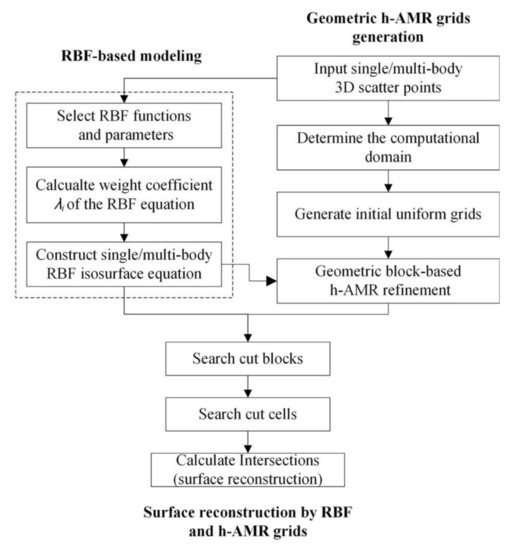
Figure 1.
Flow chart.
Specifically, the initial h-AMR Cartesian grid is generated, and its data structure is adopted throughout the work process. Meantime, the RBF implicit surface is automatically constructed by a given set of sample points. According to the characteristics of the marine structure, this work also includes the detailed comparisons of effects of uncertainty factors, which include different RBF functions and parameters, on the accuracy of results. Moreover, the RBF and h-AMR grids are combined to reconstruct the implicit isosurface and improve efficiency. We directly use the RBF equation to test whether the grid nodes of the candidate h-AMR grids are inside/outside/on the solid surface. Once the cut cells have been identified, they are subsequently refined by the h-AMR technique. Thereafter, this work combines the Newton-Raphson iterative method. Then the intersections can be iteratively calculated based on the RBF value over the h-AMR cut cells.
2.1. Spatial Discretization of Block-Based H-Adaptive Cartesian Grids
The uniform grid maintains the same grid size throughout the domain, while the h-AMR method adjusts different grid sizes in different regions. Figure 2 represents the uniform Cartesian grids (left) and the geometric h-AMR grids (right) for a 2D rectangle (blue). It can be seen that the AMR grids can reduce the total amount of grids while reaching the same grid resolution at the surface boundary.
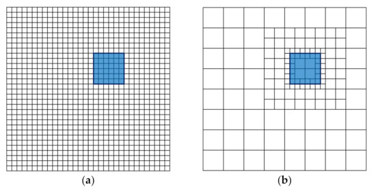
Figure 2.
(a) Uniform Cartesian grid; (b) geometric h-adaptive mesh refinement (AMR) grids (right).
The existence of multi-layered structure grids means the h-AMR grids cannot be directly indexed by the implicitly connected coordinates (i, j, k) in the uniform Cartesian grid storage. Therefore, the unstructured hierarchical tree structure needs to be adopted to store the connectivity and information on the grid of different levels.
2.1.1. Characteristics of Different h-AMR Grids
For the specific use, the proper h-AMR method needs to be selected. Depending on the grid forms stored in data tree nodes, the h-AMR can be further divided into three typical methods, the patch-based [4,26,28], cell-based [2,25,29] and block-based [30,31,32] method. Figure 3 represents the geometric refinement process of the 2D rectangle by the three typical h-AMR grid methods. Each group of grids surrounded by yellow lines forms a data tree node.
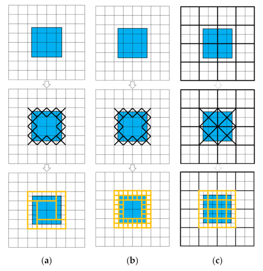
Figure 3.
Schematic diagram of three typical h-AMR geometric refinement process based on the 2D rectangle (a) patch-based; (b) cell-based; (c) block-based.
In Figure 3a, the patch-based adaptive grid consists of arbitrary rectangular patches. It needs the clustering algorithm to organize the marked cells into grid patches, and each grid patch forms a tree node. Compared with other h-AMR methods, it generates the fewest number of tree nodes. However, it may not be easy to apply the appropriate clustering algorithm [32].
The cell-based methods in Figure 3b, on the other hand, directly bisect the marked cells into ( is the space dimension) finer children cells. That makes it more flexible in refining arbitrary tagged grids. It does not need the use of clustering methods. However, due to the one-to-one correspondence between grid and tree nodes, the hierarchical data tree requires more storage capacity than a patch-based approach.
The block-based method, as illustrated in Figure 3c, has the same characteristics of the other two h-AMR methods. It includes both the grid block (heavy lines) and grid cell structures (light lines). The grid blocks are used for tagging, refining and forming tree nodes. Meanwhile, the grid cells are uniformly arranged in each grid block. The block-based h-AMR avoids the clustering procedure compared with the patch-based method. In the meanwhile, it not only retains the flexibility of the cell-based method but also partially preserves the structured grid characteristics. Therefore, this work applies the block-based h-AMR method [30]. That means the grid generation, geometric modeling, and reconstruction techniques must be fully compatible with the characteristics of the block-based h-AMR.
2.1.2. Data Structure and Grid Generation
Figure 4 shows a simple 2D block-based h-AMR grid and its data tree. In Figure 4a, the heavy lines and the light lines present the grid blocks and the grid cells, separately. After the refining procedure, the grid blocks need to be reordered, as shown in the red lines in Figure 4a. Each block is stored in the matching tree node and has a unique indexing identifier, as shown in Figure 4b. The domain (root block) forms the first tree level. The blocks without any children named leaf blocks perform the refinement and calculation. For example, in Figure 4, block 1 is the root block as well as the first data tree node located at Level 1. Block 2 (yellow) is one child of block 1, and also the parent of block 3 (purple). Block 10 (green) in Level 4 and block 3 (green) in Level 3 are both leaf blocks.
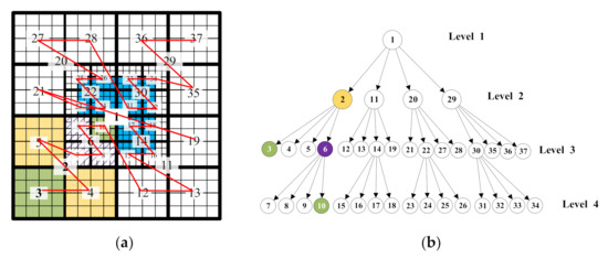
Figure 4.
Schematic diagram of a 2D block-based h-AMR grid of the 2D rectangle; (a) Geometric h-AMR grids (grid blocks: heavy lines, structured grid cells: light lines); (b) hierarchical data tree.
The grid cells are independent of the tree structure, and only participate in the practical calculations. Figure 5 represents the index of grid cells in the grid block. Each grid block contains interior structured Cartesian grid cells. They can be indexed by the implicitly connected Cartesian coordinate (i, j), where i = 1 … and j = 1 … refer to the x- and y- directions, respectively. When the number of grid cells in each block is one, the block-based method is similar to the cell-based AMR method.
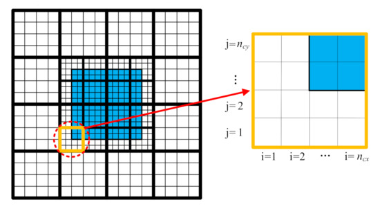
Figure 5.
Schematic diagram of index of structured grid cells (light lines) in each h-AMR block (heavy lines).
Before the simulation, the root block needs to be discretized into smaller uniform grid blocks. The initial uniform block-based h-AMR Cartesian grids are mainly controlled by three parameters, (1) the size of the computational domain (root block), (2) the coarsest refinement level of the root block, and (3) the number of the grid cells in each grid block. The initial domain contains sub-grid blocks. In this work, the computational domain size should be determined by the given scatter points. The geometric h-AMR grid layout will be further controlled by the user-defined AMR level .
2.2. RBF-Based Single/Multi-Body Geometric Modeling
2.2.1. Theory of RBF Isosurface Equation
The RBF technique uses a set of sample points to implicitly define the surface based on basis functions. This makes it feasible to model both single and multi-body geometries. The bodies in the multi-body system can be separately reconstructed by their own sample points in the same domain, as shown in Figure 6. Hence, the main operation is to construct the continuous and differentiable RBF isosurface equation for each object.
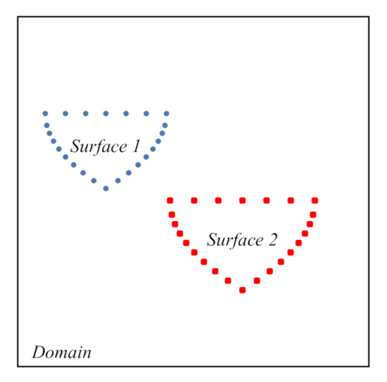
Figure 6.
Schematic diagram of scatter points of multi-body geometries in one domain.
The surface is represented by the RBF isosurface equation. Given a set of 3D distinct scatter points (also known as RBF centers), the RBF equation can be expressed as follows:
where N is the number of sample points. is the real-valued basis function, and it has various types. indicates the Euclidean distance from the space point to the given RBF center , as shown in Equation (2). is the weight coefficient to be calculated, which needs to satisfy the orthogonality in Equation (3).
Once the (), Equation (1) becomes the zero isosurface equation which represents the actual geometric surface. Equation (4) is the matrix form of Equation (1). Because of the zero terms on the right-hand side of the equation, it might lead to a trivial solution, which means that the might be zero everywhere. To avoid this, it is often necessary to add some non-zero off-surface points to the sample points. However, these additional points also increase the calculations.
2.2.2. Non-Zero Distance d
This work utilizes the constant d on the right side of the RBF equation instead of using 0. Therefore, the original number of sample points can be maintained. As shown in Figure 7, the non-zero d represents a fixed distance from the numerical surface to the actual surface.

Figure 7.
Numerical radial basis function (RBF) isosurface by adding non-zero constant d.
Thereby, we can directly calculate the non-zero scalar field. Then Equation (1) can be transformed as,
and the non-zero RBF equation for numerical calculation is represented as,
Equation (7) is the matrix notation form of Equation (6). Then the coefficient can be solved by matrix solving method such as the Gaussian elimination.
Afterward, Equation (6) can be reconstructed by the coefficient and the sample points. The actual zero-valued RBF isosurface in Equation (5) can be obtained by subtracting the distance d. In our previous 2D work [17], d = 1 is suggested. This work further validates the correctness and robustness of the distance d in the simulation.
2.2.3. RBF Functions and Shape Parameters
There are various types of functions and parameters that can be selected to construct the RBF isosurface equation. Based on our research field, this work mainly analyzes two kinds of RBFs: multiquadric RBF (MQ-RBF) and Wendland’s CSRBF.
The MQ-RBF [9] is a simple GSRBF, as represented in Equation (8), where c is the shape parameter. Frank [10] compared the scattered data interpolation algorithms and pointed out that the MQ-RBF has a better fitting result. It can be used to solve partial differential equations [33] and has been widely used in geologic modeling [6]. It has also been adopted in our previous works [17,18,19].
The capabilities and effects of MQ-RBFs are mainly controlled by the shape parameter c. The c is used as the smoothing factor to make the reconstructed surface smoother. However, if c is too large, it may cause the ill-conditioned matrix and increased numerical errors [34]. Our previous works [17,18,19] use c = 0 in hull modeling. This paper further tests two types of shape parameters c: the constant c, and the variable c of MQ-RBF. Table 1 lists some shape parameters c used in MQ-RBF.

Table 1.
Some shape parameters c in multiquadric (MQ)-RBF [10,34].
In Table 1, the constant c assigns the fixed value to all the columns of the RBF coefficient matrix. The D of Franke’s empirical formula [10] is recommended to be the smallest diameter of the bounding sphere containing all data points. For simplicity, this work uses the diagonal of the bounding box instead of D.
On the other hand, the variable c adopts different shape parameters for each matrix column according to the formula. In Table 1, the variable c in [35,36] has been applied to solve 2D function interpolations and linear boundary value problems. Here we test and compare their effects on 3D arbitrary modeling. and can be determined by Equation (9). The function in Random c is employed to produce random numbers. We should notice that the calculated pseudo-random numbers practically rely on programming languages.
Table 2 lists Wendland’s CSRBFs. The essential influencing factor of the CSRBF is the parameter continuities and the support size .

Table 2.
Wendland’s compactly supported RBF (CSRBF) of different parameter continuities.
In Table 2, means the control function of the compactly supported domain, which satisfies Equation (10). Othake [22] suggests using times the diagonal of the bounding box of the sample points as the , as shown in Equation (11). In practice, the selection of should depend on specific problems. Therefore, we analyze the uncertainty of in the simulations.
2.3. RBF-Based Geometric h-AMR and Calculation of Intersection
The RBF-based geometric modeling method is actually independent of the block-based h-adaptive Cartesian background grids. In this work, we combined them to efficiently calculate the intersections.
2.3.1. Surface Identification and RBF-Based Geometric AMR
First, the RBF isosurface equation is directly used as the geometric h-AMR criterion. Based on the value of the RBF isosurface equation, the positional relationship between an arbitrary space point and the geometric surface can be determined, as shown in Equation (12) and Figure 8.
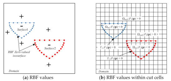
Figure 8.
Schematic diagram of RBF values inside/outside/on the multi-body isosurfaces; (a) RBF values in space; (b) RBF values in cut cells.
Since the refinement procedure is presented on the grid blocks, the next step is to find cut blocks. To help subtract the off-surface grid blocks, this work introduces the bounding box. Figure 9 represents the bounding boxes for multi-body hulls and the candidate cut blocks. As illustrated in Figure 9a, the axis-aligned rectangular region is established by the minimum and maximum coordinates of the given sample points. Additionally, the scale factor is used to properly expand the range of the object, thus avoiding the incomplete reconstruction of the geometric surface. Figure 9b represents the expanded bounding box . Here we select = 1.05 [7] in the simulations.
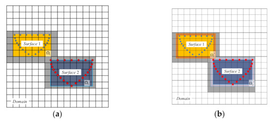
Figure 9.
Schematic diagram of bounding boxes for multi-body surfaces and the candidate cut blocks (grey); (a) Original bounding boxes; (b) Expanded bounding boxes.
Within the bounding box, the RBF value of each block node (coordinates of grid vertices; 2D: four; 3D: eight) needs to be calculated. As shown in Figure 10, once the RBF value of one node is 0, or any two nodes have opposite signs, we stop calculating the block and mark it to perform h-AMR.
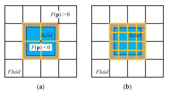
Figure 10.
(a) Uniform cut blocks (yellow lines) and RBF values of block nodes; (b) Geometric h-AMR cut blocks (yellow lines) of 2D rectangle (blue).
2.3.2. Calculation of Intersections
The next step is to calculate the intersections for geometric reconstruction. The calculation of the intersection is performed on the grid cells inside the h-AMR cut block. The method used to detect cut cells is similar to the method of cutting blocks. The difference lies in their traversal methods. The candidate cut cells are searched by the implicitly Cartesian connection. As shown in Figure 5, if the cell node is (i, j, k), its neighboring cell nodes are (i + 1, j, k), (i, j + 1, k), and (i, j, k + 1), respectively.
Due to the RBF isosurface being a continuous function, there should exist a zero-valued intersection point between the two opposite-valued nodes. Besides, with the sufficiently fine Cartesian background grid, there will be at most one intersection on each edge of the cut cell.
Figure 11a shows a 3D cut cell. is a cell node. , , and are the neighbor cell nodes of in x-, y- and z- directions, respectively. We take the intersections on the XY plan as an example, as shown in Figure 11b. Based on the RBF value, it can be seen that , , and . It indicates that is the fluid point () outside the surface, is the solid point () inside the surface, and is an intersection point on the surface. In this situation, the intersection between and needs to be calculated.
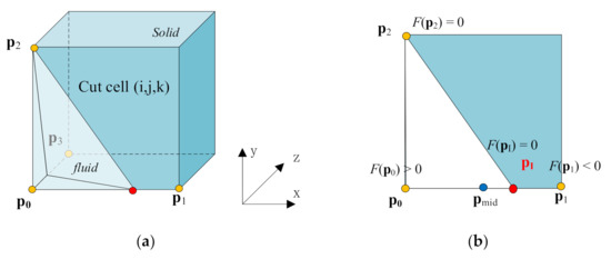
Figure 11.
(a) Schematic diagram of a 3D cut cell; (b) Intersection point on XY plan.
Based on the Newton-Raphson iterative method, the weighting coefficient s () is applied to associate with . When s = 1 ()/0 (), the intersection point becomes /, respectively. Then the coordinate of can be defined as Equation (13), in which the subscript n represents the nth iterative step.
Subsequently, we take the initial guessing value into Equation (13). This assumes the intersection is at the midpoint of the cell edge. Here we use a very small value as the convergence condition. If , Equation (14) is used to solve the in the next iterative step.
where can be calculated from Equation (15):
Equation (15) contains two conditions. If , it means is a fluid point , and the actual intersection is closer to the . Therefore, the range of reduces to , and the is replaced by the in the next iterative step. The procedure is repeatedly executed by Equations (13)–(15) until converges to .
3. Simulation and Results
This section simulates the 3D analytic geometries and practical hull forms. It includes the ellipsoidal surface, unclosed conic surface, and single/multi-body Wigley and KCS hull forms. The goal is to verify the accuracy, efficiency, and robustness of the RBF-based block-based h-AMR method. All simulations in this work use dimensionless parameters and CPU time in seconds. The numerical tests are carried out on an Intel Core i7 CPU 2.6 GHz processor.
In the simulation, we compared and analyzed the influencing factors of uncertainty in detail. In this work, the factors include: (1) the uncertainty of sample points; (2) the effect of different RBF basis functions and parameters; (3) the robustness of the non-zero distance d for RBF equation; (4) the effect of background grid size; and (5) the effectiveness and efficiency of the block-based h-AMR.
Based on the methodology, the uncertainty factor can be analyzed from two aspects: RBF implicit modeling and h-AMR-based reconstruction.
3.1. Case 1: Ellipsoidal Surface
Case 1 simulates an ellipsoidal surface. It mainly analyzes the uncertainty of influencing factors of the RBF method. Equations (16) and (17) represents the parametric equation and standard equation of the ellipsoidal surface, respectively.
is the center of the ellipsoid. In Case 1, the ellipsoid is located at the center of the computational domain. are the lengths of the principal axes. Table 3 lists the parameters of the ellipsoid and the h-AMR grids.

Table 3.
Parameters of ellipsoid and h-AMR background grids.
3.1.1. Uncertainty of Sample Points
To analyze the uncertainty of sample points, four sets of uniformly distributed sample points are selected to reconstruct the ellipsoidal surface. The sample points are obtained by the interpolation in Equation (16), and their numbers are approximately increased twofold.
Figure 12 and Figure 13 and Table 4 compare the reconstructed ellipsoidal surface and the intersection points by the MQ-RBF of c = 0 and different numbers of sample points (indicated by PS), respectively. In Table 4, PI is the number of intersections. The errors conclude the root mean square error (RMSE), mean absolute error (meanE), and maximum absolute error (maxE). TM and TR denote the time by RBF implicit modeling and the intersection calculation, respectively. TAVG indicates the reconstructed time TR consumed per intersection point. In Case 1 and Case 2, the Equation (7) is calculated by the Gaussian elimination.
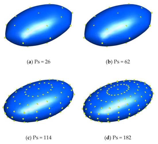
Figure 12.
Comparison of ellipsoidal RBF isosurface reconstructed by MQ-RBF of c = 0 and different numbers of sample points (yellow).
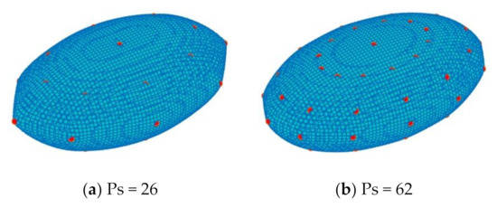
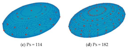
Figure 13.
Comparison of intersection points (cyan) of and different numbers of sample points (red).

Table 4.
Comparison of errors and time of ellipsoidal surface reconstructed by MQ-RBF of c = 0 and different numbers of sample points.
In Figure 12, we can see that all sets of sample points can completely reconstruct the surface. Among the four reconstructed ellipsoidal surfaces, the deformation of (a) Ps = 26 is most obvious. There is no visible difference between the results by (c) Ps = 114 and (d) Ps = 182, indicating that the results may have converged. In Table 4, even a small number of sample points can give an acceptable result: the RMSE of Ps = 26 is smaller than 5 10−2. The errors gradually decreased with the increasing number of sample points. While the number of reconstructed intersection points PI slightly increased. Moreover, by taking Figure 13 into account, this indicates that with more sample points, the reconstructed ellipsoidal surface is fuller and more convex, which leads to an increase in the number of intersections based on the same cut cell size.
On the other hand, in Table 4, TM, TR, and TAVG all increase with the number of sample points. TM is mainly cost by the construction of the coefficient matrix and the solution of the weight coefficients of the RBF equation. TR is mainly related to the number of intersections and the RBF equation. TAVG is only affected by the RBF equation. Since the increasing Ps increases the size of the RBF coefficient matrix and RBF equation, all the time increases. Based on the results, we select the PS = 62 for further discussions.
3.1.2. Validation of d
To verify the robustness of d = 1 in the RBF equation, here we analyze and compare the effect of different distances d, as shown in Table 5. The RMSE% compares the percentage of the RMSE solved by different d with d = 1.

Table 5.
Comparison of errors and time of ellipsoidal surface reconstructed by MQ-RBF of c = 0 and different distance d.
It can be seen that the errors by different d are almost the same, in which the variation of the RMSE% is smaller than 1%. This indicates that the value distance d is generally independent of the accuracy of the RBF method. Additionally, there is no considerable difference between the different TAVG and TR. When d gradually reduces, the PI slightly increases. Otherwise, the PI tends to be stable. Meantime, the reconstructed surface by d = 1 requires the lowest TM. Therefore, it is feasible to use d = 1 as a general given condition for the 3D geometric modeling and reconstruction by the MQ-RBF.
3.1.3. Uncertainty of RBF and Parameters
Table 6 and Table 7 compare the intersections reconstructed by the MQ-RBF with different shape parameters c, and the CSRBF with different continuities and support coefficients , respectively.

Table 6.
Comparison of errors and time of ellipsoidal surface reconstructed by MQ-RBF with different shape parameters c.

Table 7.
Comparison of errors and time of ellipsoidal surface reconstructed by CSRBF with different continuities and support coefficients .
In Table 7, the minimum coefficient is recommended by [22]. The RMSE% compares the percentage of the RMSE of different c with the c = 0.
From the results, we can see that both the MQ-RBF and CSRBF can successfully solve the coefficient matrix equation without singularity solutions. Since the ellipsoid is a typical smooth surface. The smaller error can indicate that the applied RBF has smooth characteristics.
In Table 6, the errors by the MQ-RBF with non-zero shape parameters are smaller than those of c = 0. It is consistent with the idea mentioned in [37] that c works to increase the smoothness and decrease the fidelity. Specifically, the fixed Franke’s empirical c and the varied Random c lead to high reconstruction accuracy, reaching 10.87% and 1.35% of the RMSE of MQ-RBF of c = 0, respectively. As to the consumption of time, the TM, and TR both slightly increase with the non-zero c. That’s because the non-zero c requires extra calculations to construct the RBF coefficient matrix. Since the Ps in Case 1 is very small, the influence of the RBF coefficient matrix on the consumed time is limited. The different TAVG are almost the same. It can be concluded that the use of non-zero c can relatively reduce the errors of the reconstructed ellipsoidal surface while increasing the TM.
In Table 7, the results by the CSRBF are very close to the MQ-RBF of c = 0. The errors of the CSRBF decrease rapidly with higher continuities (from to ), and they are even smaller than the errors of Ps = 114 and 182 in Table 4. The RMSE% of CSRBFs with continuities of ~ and are lower than 10%. It is consistent that the increase in continuities can increase the smoothness of the surface. Additionally, the errors also decrease with the increase of the support size coefficient , and then gradually converge. The magnitude of the difference between the RMSE by different is 10−4. However, in the case of using the same matrix solving method, the CSRBFs cost more TM, TAVG, and TR than the MQ-RBF of c = 0. Moreover, the TAVG slightly increases with the higher order of continuities and the larger when . That is because the CSRBF equation becomes complex with the higher continuities, thus increasing the matrix constructing time.
The results of Case 1 can verify the accuracy and effectiveness of our method for 3D surface reconstruction. In Case 1, for the MQ-RBF, Frank’s empirical c and the Random c provide better results. Besides, the CSRBF with continuities greater than can greatly smoothen the reconstructed surface but also increase the time. The increasing support size coefficient also contributes to the smoothly reconstructed surface. Taking into account the accuracy and time consumed, we only analyze the CSRBF with in further simulations.
3.2. Case 2: Unclosed Conic Surface
Normally, only the offsets of hull lines are given before hull modeling and simulation. The deck can be closed by a plane according to the draft T and depth D. Therefore, the conic surface is selected to verify the accuracy of the proposed method on the unclosed objects. It has features of a smooth surface and sharp vertex. The parametric equations and standard equations for conic surfaces are shown in Equations (18) and (19), respectively.
is the vertex coordinates of the cone at the center of the computational domain. are the length of the principal axes. Table 8 presents the parameters of the cone and the h-AMR grids.

Table 8.
Parameters of cone and h-AMR background grids.
In practical simulations we usually use a higher density of sample points in local areas, such as the fore and aft of the hull, to improve the global accuracy and fidelity of the surface. Thus here we use the unevenly distributed sample points of Ps = 401. In this case, the results mainly discuss the effect of RBFs and the influencing factors of the block-based h-AMR grids.
3.2.1. Uncertainty of RBF and Parameters
First, we analyze the effects of RBF functions and parameters on the accuracy and efficiency of the 3D unclosed surface. Based on the results of Case 1, Table 9 compares the accuracy and efficiency of the reconstructed surface by the MQ-RBF with different shape parameters c and CSRBF with different support coefficients .

Table 9.
Comparison of errors and time of cone reconstructed by MQ-RBF with different shape parameters and C2-CSRBF with different support coefficients .
In Table 9, the surface reconstructed by MQ-RBF with Franke’s c obtained a relatively higher accuracy. However, the MQ-RBF with Random c leads to significant errors, which is contradicting the results of Case 1. That indicates the MQ-RBF with Random c is not robust for the reconstruction of the 3D unclosed surface. Additionally, the smoothness of CSRBF is higher than that of MQ-RBF under different shape parameters. In the case of , the RMSE% already reaches 57.3% of the MQ-RBF of c = 0. However, since the cone has a sharp top, the smooth shape parameters of RBFs have a smaller effect on the reconstructed surface than Case 1.
On the other hand, MQ-RBF of c = 0 consumes the least time. The increment of the TM, TAVG, and TR by the MQ-RBF with non-zero c is smaller than the CSRBF. The MQ-RBF of Random c is abnormally small, indicating that it has failed to reconstruct the surface correctly and leads to an unacceptably large error. Additionally, the time consumed by the CSRBFs increases by the augment of the . Therefore, by taking consideration of the consumed time, as well as the smaller being beneficial for dispersing the coefficient matrix, we utilize the CSRBF of in further discussions.
3.2.2. Effect of Grid Size
This section tests the effect of grid cell size. Figure 14 compares the geometric block-based h-AMR grids and intersections (cyan) with sample points (red) of the cone reconstructed by different cut cell sizes. Table 10 lists the reconstructed errors and time by CSRBF of .
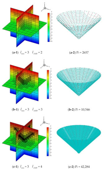
Figure 14.
Geometric h-AMR girds (grid blocks: heavy lines; grid cells: light lines) (left) and the intersection points (right) of cone reconstructed by C2- CSRBF of = 1.0 different cut cell sizes.

Table 10.
Comparison of errors and time of cone reconstructed by C2- CSRBF of = 1.0 and different cut cell sizes.
The results show that the density of grid size has a small effect on the reconstructed errors. The difference of the RMSE by different grid sizes is smaller than 5 10−4. Therefore, this proves the independence between the 3D reconstructed accuracy and the background grid size. Meantime, the generated intersections PI and the reconstructed TR increase with the increasing number of grids. The more PI can help to capture the more detailed features of the reconstructed surface.
3.2.3. Effectiveness of Geometric h-AMR Grids
To verify the effect of the block-based h-AMR on the accuracy and efficiency of 3D geometric reconstruction, we first analyze the effect of initial refinement level and AMR level on the reconstruction efficiency under the same cut cell size. The total refinement level is 6. Table 11 and Figure 15 compare the accuracy and efficiency of the reconstructed surface by CSRBF of and different . In this simulation, each grid block contains the same number of grid cells ().

Table 11.
Comparison of errors and time of cone reconstructed by C2- CSRBF = 1.0 and different AMR levels.
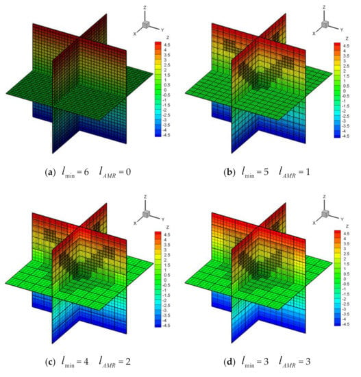
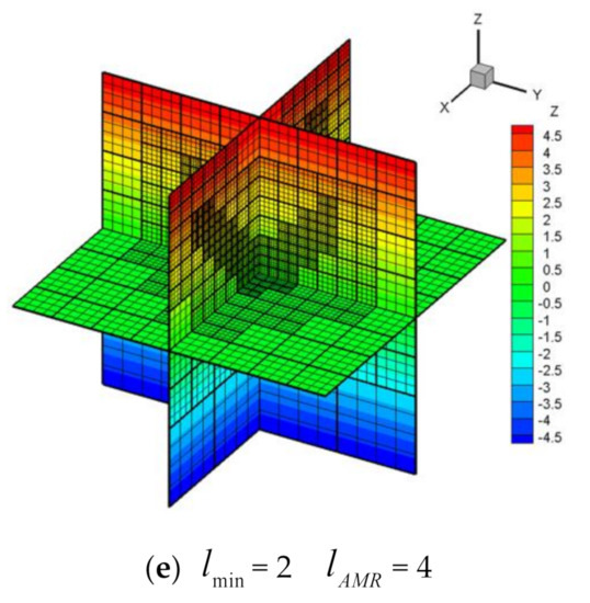
Figure 15.
Geometric h-AMR grids (grid blocks: heavy lines; grid cells: light lines) of cone reconstructed by different AMR levels.
From the results, we can see that when the cut cell size is the same and each grid block contains the same number of grid cells, the errors by different AMR levels are almost the same. This can verify the robustness of the proposed method. Additionally, the number of grid blocks, the reconstruction time TR, the initial grid generation time TIG, and the total consumed time Ttotal are generally reduced with the higher AMR levels. When = 4, the time slightly increases. It proves the effectiveness of the h-AMR procedure in improving the efficiency of 3D reconstruction problems. The layouts of grids in Figure 15d and (e) are identical. It is due to the limitation of the block-based h-AMR grid that the gap of the level of adjacent blocks is not bigger than 1. Thus, the different AMR levels may result in an identical final h-AMR background grid.
Furthermore, we compare the accuracy and the efficiency of the cone by different numbers of grid cells contained in each grid block, as illustrated in Table 12 and Figure 16. Except for the uniform grid cell in initial level 1, the other h-AMR grid cells use the initial level 3. The cut cell size remains the same.

Table 12.
Comparison of errors and time of cone reconstructed by C2- CSRBF = 1.0 and different number of grid cells.
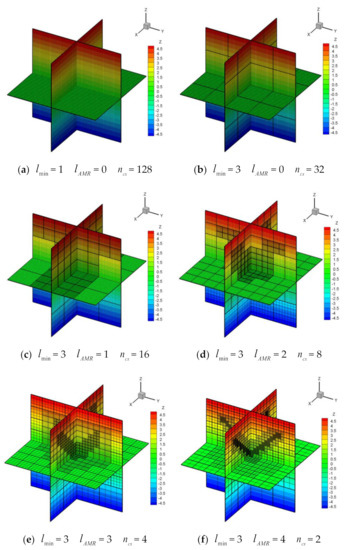
Figure 16.
Geometric h-AMR grids (grid blocks: heavy lines; grid cells: light lines) of cone reconstructed by different numbers of grid cells.
It can be seen from Table 12 that the errors are almost the same. The total refinement levels and block numbers correspondingly increase by the reducing number of grid cells. Additionally, TR decreases by the reduced number of grid cells. When the number of grid cells decreases from to , the time slightly increases. This proves the block-based h-AMR process can improve the reconstructed efficiency compared with the uniform Cartesian grid. Meantime, it also indicates that the increasing number of grid cells in each grid block can generally increase the flexibility and the reconstructed efficiency of the h-AMR procedure but requires more computer storage resources. Therefore, the following simulation uses the = .
3.3. Case 3: Wigley Hull Form
In case 3, we simulate the Wigley hull to verify the effectiveness and efficiency of the proposed method for the practical ship reconstruction. As a general-purpose mathematical ship type, the Wigley hull has a simple hull form, and the body can be represented by a cluster of parabolas. It has a sharp bottom, aft, and fore, in which the fore and aft profiles are symmetrical. Equation (20) shows the exact mathematical expression of the Wigley hull.
where is the length of the waterline, B is the beam, and T is the draught. They refer to the x-, y-, and z- directions, respectively. In Case 3, = 0.1 and = 1.6. The main dimensions of the Wigley hull and the parameters of h-AMR background grids are represented in Table 13.

Table 13.
Main dimensions of Wigley hull and parameters of h-AMR background grids.
The given hull offsets are usually unclosed. In this work, we directly reconstruct the hull body by the unclosed sample points and the Boolean operation rather than adding additional deck points.
3.3.1. Geometric Modeling
According to the workflow in Figure 1, the sample points need to be determined first. Figure 17 shows the RBF isosurface of the Wigley hull by the MQ-RBF of c = 0 and two sets of sample points. Since the initial offset points of ships are usually not enough for accurate implicit modeling, the two sets of sample points are both obtained by interpolation from the original offsets.
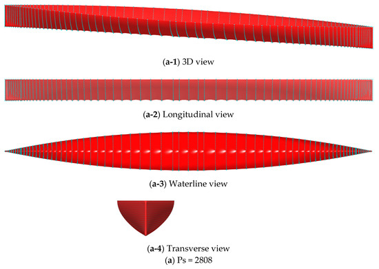
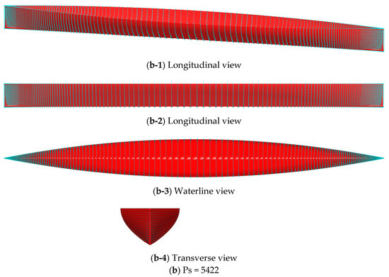
Figure 17.
3D view, longitudinal view, waterline view and transverse view of Wigley hull implicit model (red) with sample points (cyan); (a) Ps = 2808; (b) Ps = 5422.
In Figure 17, we can see that both sets of sample points can result in the correct reconstruction of the Wigley hull. However, due to the relatively sparse given points, the surface reconstructed by (a) Ps = 2808 sample points is comparatively not smooth at the midship section. Its waterline profile shows pronounced depression. By using the (b) Ps = 5422 sample points, the distortion of the reconstructed surface can be clearly reduced.
3.3.2. Surface Reconstruction
The following procedure is to generate the geometric block-based h-AMR grid and to calculate the intersection points. The computational domain (root grid block) covering the Wigley hull is generated based on the hull offsets, and then it is discretized into the initial uniform grid blocks. Based on the RBF isosurface generated by the two sets of sample points, we can obtain two layouts of geometric h-AMR grids, as illustrated in Figure 18.
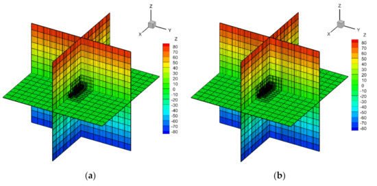
Figure 18.
Geometric h-AMR grids (grid blocks: heavy lines; grid cells: light lines) of the Wigley hull by two sets of sample points; (a) Ps = 2808; (b) Ps = 5422.
Table 14 compares the errors and time of the Wigley hull reconstructed by the MQ-RBF of c = 0 and two sets of given points. In practical simulations of Case 3 and Case 4, Equation (7) in modeling time TM is calculated by the built-in matrix solver function in MATLAB. The results again show that the number of sample points has a great impact on the accuracy of the reconstruction and the consumed time. To validate the effect of different kinds of RBFs on the accuracy of the reconstructed surface, Ps = 5422 is selected for further analysis.

Table 14.
Comparison errors and time of Wigley hull reconstructed by two sets of sample points.
Based on the results of the previous cases, we select three RBFs: the MQ-RBF of c = 0, the Franke’s empirical c, and the CSRBF of to compare the errors and time of the intersection points, as illustrated in Table 15. Figure 19 and Figure 20 compares the RBF isosurfaces and intersections within the bounding box of the Wigley hull reconstructed by the three RBFs.

Table 15.
Comparison of errors and time of Wigley hull reconstructed by three RBFs.
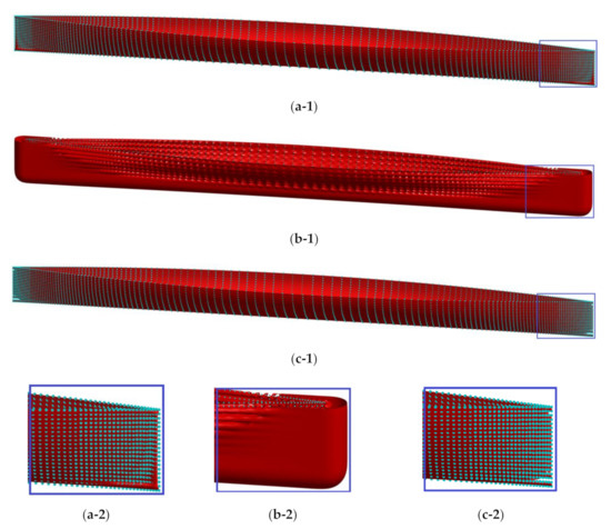
Figure 19.
Comparison RBF isosurfaces (red) and sample points (cyan) of Wigley hull by three RBFs (up) and their enlarged bow surface (down); (a) MQ-RBF of c = 0; (b) MQ-RBF of Franke’s c; (c) CSRBF of = 1.0.
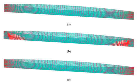
Figure 20.
Intersections (cyan) and sample points (red) of Wigley hull reconstructed by three RBFs; (a) MQ-RBF of c = 0; (b) MQ-RBF of Franke’s c; (c) CSRBF of = 1.0.
From the results, we can see that the MQ-RBF of c = 0 completely reconstructs the Wigley hull with acceptable errors. It also costs the least TM and TR. Franke’s empirical c produces remarkable errors compared with the MQ-RBF of c = 0. That is because the formula of Franke’s empirical c is related to the distribution and the diameter of the enclosing sphere of the sample points. Since the hull has the unclosed sample points and a large aspect ratio, the effectiveness of Franke’s empirical c has been affected.
On the other hand, the CSRBF of has the smallest RMSE but the reconstructed surface has some tiny leaks at the aft and bow, as shown in Figure 19c-2. This indicates that most of the 3D Wigley hull has the characteristics of convexity and smoothness. However, due to the sharp aft and bow, the reconstruction contains local inaccuracies by using the smoother RBF function. Meantime, the CSRBF costs the most TM and TR. Overall, the MQ-RBF with c = 0 provides not only relatively highly accurate results but also stability and robustness.
3.4. Case 4: Multi-Body Hull Forms
In this section, we further validate the accuracy and efficiency of our method on 3D multi-body hull problems. The system includes the Wigley and KCS hulls. The KCS hull is the modern container ship with a bulbous bow and transom stern. The curvature of the bow and stern changes greatly compared with the hull body. It has been widely used in CFD verification. To commonly reconstruct the Wigley hull and the KCS hull, the computational domain should cover both sets of sample points. Table 16 lists the main dimensions of the KCS hull and the parameters of the h-AMR grids.

Table 16.
Main dimensions of KCS hull and parameters of multi-body h-AMR background grids.
3.4.1. Single KCS Hull Modeling
First, we analyze the effect of the RBF function on the single KCS hulls, as shown in Figure 21.
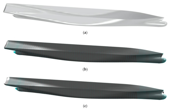
Figure 21.
Comparison of KCS hull models (a) Standard explicit model; (b) Implicit model by MQ-RBF of c = 0; (c) Implicit model by C2- CSRBF of = 1.0.
Based on the results of Case 3, Figure 21 compares the KCS standard explicit model and implicit RBF models reconstructed by MQ-RBF of c = 0 and CSRBF of , respectively. It can be seen that there is no visible difference between the standard ship explicit model (a) and the implicit model by the MQ-RBF of c = 0 (b). However, our method only utilizes the scatter points for automatic modeling, which reduces the manual operation in explicit modeling. Besides, the implicit surface by the CSRBF is smoother, except for the stern and bow which have local incorrect redundant fragments. That is because the CSRBF possesses relatively high smoothness and convexity but the curvatures of the bow and stern of the KCS hull contain both concave and convex features. By comparison, the MQ-RBF of c = 0 provides higher fidelity. Therefore, we select the MQ-RBF of c = 0 to simulate the multi-hull system.
3.4.2. Multi-body Hulls Modeling
Figure 22 represents the RBF isosurface and the sample points of the multi-body hull system. We can see that the multi-body system consists of multi-scale hull forms, and each hull is consistent with the corresponding single hull model. Due to the flexibility of the RBF modeling method, every single body can be separately reconstructed by the individual RBF function. Based on the previous results, we use MQ-RBF of c = 0 for both hulls in the multi-body system.
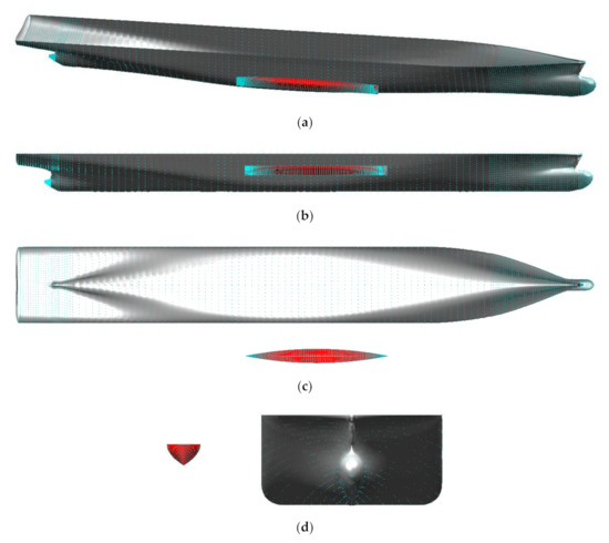
Figure 22.
Implicit multi-body hull models with sample points (cyan): Wigley hull (red) and KCS hull (grey); (a) 3D view; (b) Longitudinal view; (c) Waterline view; (d) Transverse view.
3.4.3. Multi-body Hulls Reconstruction
For the multi-body system, every single object generates its bounding box from a different set of sample points. Subsequently, the background grids within each bounding box can be locally refined through the separate RBF model and AMR levels. Figure 23 illustrates the geometric h-AMR grids of the multi-body hulls. It can be seen that each grid set follows the corresponding hull shape.
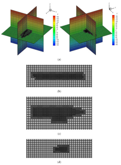
Figure 23.
Geometric h-AMR grids (grid blocks: heavy lines; grid cells: light lines) of multi-body hull system; (a) 3D view; (b) Longitudinal view; (c) Waterline view; (d) Transverse view.
Figure 24 represents the intersection points of the multi-body hulls. Specifically, we compare the errors and time between the multi-body hulls and the previous single hull, as shown in Table 17. From Table 17, it can be seen that the number of intersections PI of the comparative group is identical, and the reconstruction time TR and average reconstruction time TAVG are quite similar. The errors of the two Wigley hulls are very similar, in which the difference of the RMSE is at 10−5 order magnitude. It also demonstrates the independence of the h-AMR background grids from the RBF model in surface reconstruction. Additionally, Figure 25 compares the typical cross-sections of the KCS hull, and the intersections are consistent with the sample points. Therefore, Case 4 verifies the accuracy and robustness of the proposed method to solve the multi-body reconstruction problem.
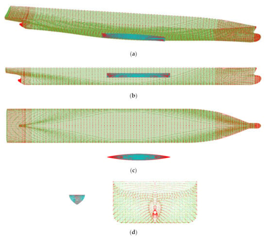
Figure 24.
Intersection points of the multi-body hulls with sample points (red): Wigley hull (cyan) and KCS hull (green); (a) 3D view; (b) Longitudinal view; (c) Waterline view; (d) Transverse view.

Table 17.
Comparison of errors and time of single hull and multi-body hulls.
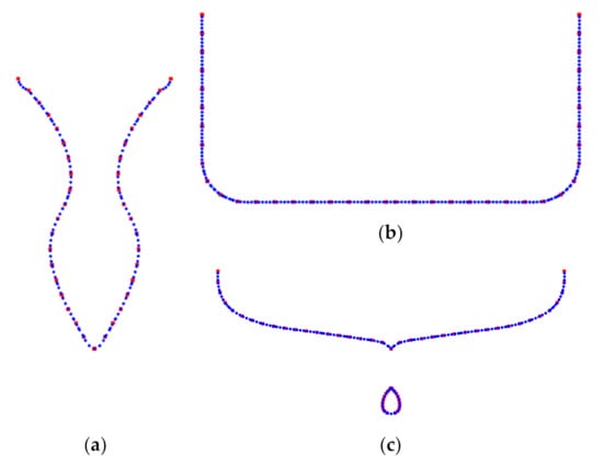
Figure 25.
Comparison of the reconstructed typical cross-sections (blue) of KCS hull in multi-body system with sample points (red); (a) Bow; (b) Midship; (c) Stern.
4. Discussion and Conclusions
This work designs an RBF-based h-adaptive refinement Cartesian grid method for modeling and reconstructing the complex single/multi-body geometries in ship and ocean engineering. The RBF technique is adopted within the non-body-fitted Cartesian background grid framework, in which the block-based h-AMR approach is utilized instead of the uniform Cartesian grid. Thus the accuracy of the geometric boundary can be improved, and the computational overhead can also be avoided. By combining the h-AMR grids, the RBF has achieved three functions, including the geometric modeling, geometric h-AMR grid indicator, and intersection calculation.
First, by giving the specific sets of scatter points, such as the unclosed ship offsets, the arbitrary single/multi-body RBF isosurface can be directly reconstructed without the need for additional manual operations. The usage of non-zero distance d = 1 keeps the number of samples in the RBF isosurface equation the same. Subsequently, within the automatically generated bounding box, the cut blocks and its cut cells can be searched and refined according to RBF equation value. Afterward, the Newton-Raphson iterative method is implemented to calculate the potential intersections between the h-AMR grids and the RBF isosurface. The effectiveness and robustness of the proposed method are validated by simulating the 3D analytical geometries and the practical single/multi-body hulls. The robustness of the non-zero distance d = 1 is also proved. Additionally, based on the characteristics of marine structures, the influencing factors of the proposed method are discussed in detail, including the number of sample points, RBF basis functions and parameters, grid size, and geometric h-AMR process.
The results are analyzed by the view of the RBF technique and the h-AMR background grids, respectively. For the RBF modeling method, the number of sample points PS is critical to the completeness and correctness of the reconstructed surface. Meantime, due to the characteristics of the RBF equation, the increasing number of sample points will also obviously increase the modeling time TM, and slightly cost more reconstruction time TR and average reconstruction time TAVG. That is due to the construction of the RBF equation and the matrix solving procedure. Additionally, under a certain number of sample points, using the appropriate parameters and RBFs can further improve the reconstruction accuracy. The main influencing factors include the shape parameters c for the MQ-RBF, the parameter continuities, and support coefficient for the CSRBF. The non-zero shape parameters c provides the higher smoothness than c = 0. They will also cost more time due to the more complex coefficient matrix of the RBF equation, where the effect on the TR is smaller than the TM. Among non-zero c, Franke’s empirical c is stable for reconstructing the smooth surface with uniformly distributed sample points. For the CSRBFs, the results of the CSRBF are close to the MQ-RBF of c = 0. The CSRBFs with higher continuities and the can remarkably improve the accuracy of smooth surfaces. However, as for the objects containing sharp features, this smoothness and convexity will blur the sharp features and reduce the fidelity. Besides, within the same matrix solving methods, the CSRBFs will consume more TM, TR and TAVG compared with the MQ-RBFs. It can be concluded that the most concise, robust, and automatic way to model ship structures is to utilize the MQ-RBF with c = 0. It has high fidelity and is ideal for surface containing sharp features, or objects having both concave and convex curvatures. It also takes the least time.
On the other hand, the grid has a small effect on reconstruction accuracy. This proves the independence of the RBF technique from the background grid. Specifically, the finer grid size can describe more details of surface features. It also costs more TR due to the increase in intersection calculation. Besides, the effectiveness of the geometric block-based h-AMR grids is also validated. The h-AMR technique can maintain accuracy while reducing the time consumed compared with the uniform Cartesian grids. Meanwhile, within the same cut cell size, the TR can be reduced by using the higher x and the smaller number of grid cells in each grid block in a certain range.
Overall, the proposed RBF-based h-adaptive refinement Cartesian grid method is accurate, automatic, robust, and efficient for arbitrary single/multi-body geometric modeling and reconstruction. It only needs the given set of scatter points to simulate the surface, and the results are reproducible. In addition, we found the MQ-RBF of c = 0 is more robust and suitable to handle the complex single/multi-body hull structures containing sharp and smooth features. The method can be easily employed in other marine structures and other engineering fields. However, the traditional way to solve RBF is computationally expensive. In further research, we will focus on the local RBF technique. It can help reduce the geometric modeling time TM. Meantime, it is also possible to use the specific RBF in different areas, allowing for an improvement in local smoothness/convexity or high fidelity depending on the surface features.
Author Contributions
Conceptualization, methodology, results and writing, L.M.; review, editing and supervision, T.L. All authors have read and agreed to the published version of the manuscript.
Funding
The present work is supported by the Major International Joint Research Project of the National Science Foundation of China (No. 51720105011), the Major Project of the Field Fund of China (No. 61402070105), the National Science Foundation of China (No. 51579196), and the Fundamental Research Funds for the Central Universities (2016-YB-013).
Informed Consent Statement
Not applicable.
Data Availability Statement
The data presented in this study is available on request from the corresponding author. The data is not publicly available because it is part of the results of the funds.
Acknowledgments
The authors would like to thank the anonymous reviewers and academic editor for their valuable comments and suggestions.
Conflicts of Interest
The authors declare no conflict of interest. The funders had no role in the design of the study; in the collection, analyses, or interpretation of data; in the writing of the manuscript, or in the decision to publish the results.
References
- Zheng, Y.; Chen, J. Unstructured Mesh Generation: Theories, Algorithms and Applications; Science Press: Beijing, China, 2016; pp. 218–219. [Google Scholar]
- DeZeeuw, D.; Powell, K.G. An Adaptively Refined Cartesian Mesh Solver for the Euler Equations. J. Comput. Phys. 1993, 104, 56–68. [Google Scholar] [CrossRef]
- Ma, L.; Li, T.; Xin, J.; Zhou, S.; Lin, Z. Development Review of H-Adaptive Cut-Cell Method in the Field of Ship and Ocean Engineering. Wuhan Ligong Daxue Xuebao (Jiaotong Kexue Yu Gongcheng Ban)/J. Wuhan Univ. Technol. (Transp. Sci. Eng.) 2018, 42, 422–429. [Google Scholar] [CrossRef]
- Berger, M.J.; Oliger, J. Adaptive Mesh Refinement for Hyperbolic Partial Differential Equations. J. Comput. Phys. 1984, 53, 484–512. [Google Scholar] [CrossRef]
- Kuo, Y.L.; Cleghorn, W.L.; Behdinan, K.; Fenton, R.G. The H-p-r-Refinement Finite Element Analysis of a Planar High-Speed Four-Bar Mechanism. Mech. Mach. Theory 2006, 41, 505–524. [Google Scholar] [CrossRef]
- Hillier, M.J.; Schetselaar, E.M.; de Kemp, E.A.; Perron, G. Three-Dimensional Modelling of Geological Surfaces Using Generalized Interpolation with Radial Basis Functions. Math. Geosci. 2014, 46, 931–953. [Google Scholar] [CrossRef]
- Tobor, I.; Reuter, P.; Schlick, C. Efficient Reconstruction of Large Scattered Geometric Datasets Using the Partition of Unity and Radial Basis Functions. WSCG 2004, 12, 467–474. [Google Scholar]
- Huang, Z.; Carr, N.; Ju, T. Variational Implicit Point Set Surfaces. ACM Trans. Graph. 2019, 38. [Google Scholar] [CrossRef]
- Hardy, R.L. Multiquadric Equations of Topography and Other Irregular Surfaces. J. Geophys. Res. 1971, 76, 1905–1915. [Google Scholar] [CrossRef]
- Franke, R. Scattered Data Interpolation: Tests of Some Methods. Math. Comput. 1982, 38, 181–200. [Google Scholar] [CrossRef]
- Zhong, D.; Zhang, J.; Wang, L. Fast Implicit Surface Reconstruction for the Radial Basis Functions Interpolant. Appl. Sci. 2019, 9, 5335. [Google Scholar] [CrossRef]
- De Araújo, B.R.; Lopes, D.S.; Jepp, P.; Jorge, J.A.; Wyvill, B. A Survey on Implicit Surface Polygonization. ACM Comput. Surv. 2015, 47. [Google Scholar] [CrossRef]
- Majdisova, Z.; Skala, V. Radial Basis Function Approximations: Comparison and Applications. Appl. Math. Model. 2017, 51, 728–743. [Google Scholar] [CrossRef]
- Cervenka, M.; Skala, V. Behavioral Study of Various Radial Basis Functions for Approximation and Interpolation Purposes. In Proceedings of the 2020 IEEE 18th World Symposium on Applied Machine Intelligence and Informatics (SAMI), Herlany, Slovakia, 23–25 January 2020; pp. 135–140. [Google Scholar] [CrossRef]
- Huang, F.; Yang, C. Hull Form Optimization of a Cargo Ship for Reduced Drag. J. Hydrodyn. 2016, 28, 173–183. [Google Scholar] [CrossRef]
- Cheng, X.; Feng, B.; Liu, Z.; Chang, H. Hull Surface Modification for Ship Resistance Performance Optimization Based on Delaunay Triangulation. Ocean Eng. 2018, 153, 333–344. [Google Scholar] [CrossRef]
- Ye, J.; Li, T.; Price, W.G.; Temarel, P. Numerical Simulations of a Moving Multibody Using a Two-Phas Solver. In Proceedings of the The Twenty-fourth International Ocean and Polar Engineering Conference, Busan, Korea, 15–20 June 2014; pp. 666–673. [Google Scholar]
- Zhou, S.; Li, T.; Jin, Q.; Price, W.G.; Temarel, P.; Hudson, D.A. Geometric Modeling over a Background Cartesian Grid Using Radial Basis Functions. In Proceedings of the 27th International Ocean and Polar Engineering Conference, San Francisco, CA, USA, 25–30 June 2017; pp. 609–614. [Google Scholar]
- Ma, L.; Li, T.; Liu, Z.; Shao, J.; Wu, H.; Price, W.G.; Temarel, P.; Hudson, D.A. Geometric Modeling and Mesh Generation by Radial Basis Functions and Their Application to Ship Flow Simulations. In Proceedings of the 29th International Ocean and Polar Engineering Conference, Honolulu, HI, USA, 16–21 June 2019; Volume 3, pp. 2849–2856. [Google Scholar]
- Ban, D.; Ljubenkov, B. Global Ship Hull Description Using Single RBF. In Towards Green Marine Technology and Transport; Guedes Soares, C., Dejhalla, R., Pavletic, D., Eds.; CRC Press: Boca Raton, FL, USA, 2015; pp. 457–464. [Google Scholar] [CrossRef]
- Wendland, H. Piecewise Polynomial, Positive Definite and Compactly Supported Radial Functions of Minimal Degree. Adv. Comput. Math. 1995, 4, 389–396. [Google Scholar] [CrossRef]
- Ohtake, Y.; Belyaev, A.; Seidel, H.P. A Multi-Scale Approach to 3D Scattered Data Interpolation with Compactly Supported Basis Functions. In Proceedings of the SMI 2003: Shape Modeling International 2003, Seoul, Korea, 12–15 May 2003; pp. 153–161. [Google Scholar] [CrossRef]
- Kojekine, N.; Hagiwara, I.; Savchenko, V. Software Tools Using CSRBFs for Processing Scattered Data. Comput. Graph. 2003, 27, 311–319. [Google Scholar] [CrossRef]
- Aftosmis, M.J. Solution Adaptive Cartesian Grid Methods for Aerodynamic Flows with Complex Geometries. In 28th Computational Fluid Dynamics; Lecture Series; NTRS: Washington, DC, USA, 1997. [Google Scholar]
- Lorensen, W.E.; Cline, H.E. Marching Cubes: A High Resolution 3D Surface Construction Algorithm. In Proceedings of the 14th Annual Conference on Computer Graphics and Interactive Techniques, SIGGRAPH 1987, New York, NY, USA, 27–31 July 1987; pp. 163–169. [Google Scholar] [CrossRef]
- Popinet, S. Gerris: A Tree-Based Adaptive Solver for the Incompressible Euler Equations in Complex Geometries. J. Comput. Phys. 2003, 190, 572–600. [Google Scholar] [CrossRef]
- Zhang, W.; Almgren, A.; Beckner, V.; Bell, J.; Blaschke, J.; Chan, C.; Day, M.; Friesen, B.; Gott, K.; Graves, D.; et al. AMReX: A Framework for Block-Structured Adaptive Mesh Refinement. J. Open Source Softw. 2019, 4, 1370. [Google Scholar] [CrossRef]
- Adams, M.; Colella, P.; Graves, D.T.; Johnson, J.N.; Johansen, H.S.; Keen, N.D.; Ligocki, T.J.; Martin, D.F.; McCorquodale, P.W.; Modiano, D.; et al. Chombo Software Package for AMR Applications Design Document. 2015. Available online: http://seesar.lbl.gov/ANAG/chombo (accessed on 21 August 2014).
- Wu, S.; Zhang, J.; Xiao, Q.; Ni, M.-J. Comparison of Two Interfacial Flow Solvers: Specific Case of a Single Droplet Impacting onto a Deep Pool. Comput. Math. Appl. 2020. [Google Scholar] [CrossRef]
- MacNeice, P.; Olson, K.M.; Mobarry, C.; De Fainchtein, R.; Packer, C. PARAMESH: A Parallel Adaptive Mesh Refinement Community Toolkit. Comput. Phys. Commun. 2000, 126, 330–354. [Google Scholar] [CrossRef]
- Fryxell, B.; Olson, K.; Ricker, P.; Timmes, F.X.; Zingale, M.; Lamb, D.Q.; MacNeice, P.; Rosner, R.; Truran, J.W.; Tufo, H. FLASH: An Adaptive Mesh Hydrodynamics Code for Modeling Astrophysical Thermonuclear Flashes. Astrophys. J. Suppl. Ser. 2000, 131, 273–334. [Google Scholar] [CrossRef]
- Van Der Plas, P.; Veldman, A.E.P.; Van Der Heiden, H.J.L.; Luppes, R. Adaptive Grid Refinement for Free-Surface Flow Simulations in Offshore Applications. In Proceedings of the International Conference on Offshore Mechanics and Arctic Engineering—OMAE, St. John’s, NL, Canada, 31 May–5 June 2015; Volume 2. [Google Scholar] [CrossRef]
- Ku, C.-Y.; Liu, C.-Y.; Xiao, J.-E.; Hsu, S.-M. Multiquadrics without the Shape Parameter for Solving Partial Differential Equations. Symmetry 2020, 12, 1813. [Google Scholar] [CrossRef]
- Fallah, A.; Jabbari, E.; Babaee, R. Development of the Kansa Method for Solving Seepage Problems Using a New Algorithm for the Shape Parameter Optimization. Comput. Math. Appl. 2019, 77, 815–829. [Google Scholar] [CrossRef]
- Xiang, S.; Wang, K.M.; Ai, Y.; Sha, Y.D.; Shi, H. Trigonometric Variable Shape Parameter and Exponent Strategy for Generalized Multiquadric Radial Basis Function Approximation. Appl. Math. Model. 2012, 36, 1931–1938. [Google Scholar] [CrossRef]
- Afiatdoust, F.; Esmaeilbeigi, M. Optimal Variable Shape Parameters Using Genetic Algorithm for Radial Basis Function Approximation. Ain Shams Eng. J. 2015, 6, 639–647. [Google Scholar] [CrossRef]
- Pouderoux, J.; Tobor, I.; Gonzato, J.C.; Guitton, P. Adaptive Hierarchical RBF Interpolation for Creating Smooth Digital Elevation Models. In Proceedings of the GIS—The ACM International Symposium on Advances in Geographic Information Systems 2004, Washington, DC, USA, 12–13 November 2004; pp. 232–240. [Google Scholar] [CrossRef]
Publisher’s Note: MDPI stays neutral with regard to jurisdictional claims in published maps and institutional affiliations. |
© 2020 by the authors. Licensee MDPI, Basel, Switzerland. This article is an open access article distributed under the terms and conditions of the Creative Commons Attribution (CC BY) license (http://creativecommons.org/licenses/by/4.0/).