Comparison of Simulations with a Mean-Field Approach vs. Synthetic Correlated Networks

Abstract

It is well known that dynamical processes on complex networks are influenced by the degree correlations. A common way to take these into account in a mean-field approach is to consider the function $k_{nn}\left(k\right)$ (average nearest neighbors degree). We re-examine the standard choices of $k_{nn}$ for scale-free networks and a new family of functions which is independent from the simple ansatz $k_{nn}\propto k^{\alpha }$ but still displays a remarkable scale invariance. A rewiring procedure is then used to explicitely construct synthetic networks using the full correlation $P(h\mid k)$ from which $k_{nn}$ is derived. We consistently find that the $k_{nn}$ functions of concrete synthetic networks deviate from ideal assortativity or disassortativity at large k. The consequences of this deviation on a diffusion process (the network Bass diffusion and its peak time) are numerically computed and discussed for some low-dimensional samples. Finally, we check that although the $k_{nn}$ functions of the new family have an asymptotic behavior for large networks different from previous estimates, they satisfy the general criterium for the absence of an epidemic threshold.

1. Introduction

As is nowadays well known, a large variety of real-world networks display a scale-free property, see, e.g., in [1,2,3,4]. A further feature typically found to be present for example in social networks is represented by assortative mixing, see, e.g., in [2,5]. This expresses the tendency of nodes to be connected with nodes which are similar to them. In particular, degree assortativity—which, at least in the mathematical and physical literature, provides the most studied example of assortativity—suggests that high degree nodes are preferentially linked to other high degree nodes and low degree nodes to other low degree nodes. The opposite property, degree disassortativity, according to which hubs are preferentially connected to small-degree nodes, and vice versa, is present in general in biological and technological networks, see, e.g., in [2,5]. Networks which exhibit assortativity or disassortativity are said to be correlated.

In this paper, we explore some aspects of different possible mathematical and computational approaches to the treatment of evolutionary systems defined on this kind of networks. We are ultimately motivated by the interest for the dynamics of phenomena pertaining to a socio-economic context. An effective formulation of the evolution equations describing such phenomena cannot neglect the nature of the links among the elements of the systems at hand. Given that the incorporation of the network of connections can be achieved with different approaches, it is natural to analyze which are the advantages and which are prices and costs of each approach.

To fix ideas, we consider here the problem of diffusion of innovations, for which two of the possible formal frameworks are briefly recalled. Both frameworks are expressed by systems of differential equations. One of them mimics the heterogeneous mean-field approach developed and successfully applied by Boguñá, Pastor-Satorras, and Vespignani for the investigation of epidemic spreading in complex networks, see, e.g., in [6,7]. It involves a number of equations equal to the maximum degree n of the nodes in the network. The other framework relies on the explicit construction of an ensemble of networks; for each element of the ensemble, a much larger system of N differential equations is studied, N being the number of nodes in the network. The construction of the ensemble involves a rewiring procedure: starting from an initial network configuration, links between nodes are repeatedly detached and reattached in such a way that the degree distribution is preserved. Various algorithms exist for the generation of arbitrarily two-points correlated networks, or maximally assortative or maximally disassortative networks, see, e.g., in [8,9,10,11,12], and we employ here one of them.

Our investigation aims at a comparison of the different approaches outlined above. The results obtained reveal facets and patterns, which we think worthwhile to illustrate.

As complex networks are in fact ubiquitous (playing an important role in communications infrastructure, in human and social relations, in protein interactions, in transport structures, in neural circuits, and much more), the unprecedented data availability and computing power achieved in the last two decades has been fostering a tremendous number of investigations and works in the field. A wide range of different issues are tackled in these works, relative, for example, to empirical observations, statistical and structural properties, modeling and algorithmic construction and, to a lesser extent, to dynamical processes taking place on top of networks. As a reference for recent contributions, containing in turn a whole set of further references, we suggest here the two volumes [13]. Yet, in spite of several advancements and progresses, much remains to be done and understood. In particular, the main purpose of this paper is to contribute to a better comprehension of theoretical and foundational aspects concerning assortative scale-free networks and their role for the mathematical modeling of systems with social interaction. Current work in this direction objectively displays some research gaps, because on one side quantities like the correlation coefficient r and the average nearest neighbor degree function $k_{nn}\left(k\right)$ (see below the definitions) can be measured for real networks without any ambiguity; on the other hand, formal models based on a mean-field approach move from strong assumptions on the form of $k_{nn}\left(k\right)$ without questioning whether such assumptions can be realized on assortative scale-free networks at least at the level of construction algorithms. In this work, we make an effort to bridge the gaps between mean-field and real networks. This is also clearly relevant in terms of applicability, because if one wants to simulate dynamical processes or diffusion processes on a certain kind of network, the first technical choice one encounters is whether to describe the network through the adjacency matrix of the nodes or the correlation functions of their degrees.

The rest of the paper is organized as follows. In Section 2, we recall the methods usually employed to analyze degree correlation properties. Section 3 is devoted to the average nearest neighbor degree function $k_{nn}\left(k\right)$. Aspects of the behavior of this function are described, based on outputs of simulations relative to networks of various dimensions, both as obtained in a mean-field framework and for concrete cases. The resulting differences are outlined and discussed. In particular, five assortative networks families, and a disassortative one, are considered. In Section 4, the effects of assortative mixing and of the two different approaches mentioned above on the diffusion dynamics and related peak times are explored. Section 5 contains remarks on a further indicator, the average of the average nearest neighbor degree function. It provides as well a couple of relations involving $k_{nn}\left(k\right)$ and some moments of the degree distribution which can be useful towards calculating certain indices of interest in the present context. Finally, in Section 6 we discuss our results.

These include the detection of an unexpected quasi-invariance property of the graph shape of the function $k_{nn}\left(k\right)$ (calculated through the correlation coefficients) with respect to the network maximal degree; the construction of correlated networks whose function $k_{nn}\left(k\right)$ does not behave, as generally expected in the literature, as $\alpha k^{\beta }$ for some coefficient $\alpha$ and $\beta$; and a qualitative agreement between the estimates of diffusion peak times obtained with the two different methods employed.

2. Measuring Assortative and Disassortative Mixing

We focus here on scale-free complex networks whose degree distribution is given (for $1\le k\le n$, with $n\in \mathbf{N}$) by $P\left(k\right)=c/k^{\gamma }$ for some $\gamma \in (2,3)$ and some positive constant c determined by the normalization ${\displaystyle \sum _{k=1}^n}P\left(k\right)=1$. Two frequently used tools to detect assortativity or disassortativity are the correlation coefficient r introduced by Newman in [14] and the average nearest neighbor degree function $k_{nn}\left(k\right)$ [15]. This function is defined in terms of the correlation coefficients $P(h\mid k)$, where $P(h\mid k)$ denotes for $1\le h,k\le n$ the conditional probability for a node of degree k to be connected to a node of degree h. Indeed, it is given by

$$k_{nn}\left(k\right)=\sum _{h=1}^{n}hP(h\mid k),$$

(1)

with the $P(h\mid k)$ satisfying for all $h,k=i=1,\cdots ,n$:

$$P(h\mid k)\ge 0,\sum _{h=1}^{n}P(h\mid k)=1,$$

(2)

and the “Network Closure Condition”

$$hP(k\mid h)P\left(h\right)=kP(h\mid k)P\left(k\right).$$

(3)

If $k_{nn}\left(k\right)$ is increasing in k, the network is assortative and if $k_{nn}\left(k\right)$ is decreasing in k, the network is disassortative. On the other hand, the coefficient r is defined as

$$r=\frac{1}{{\sigma }_q^2}\sum _{k,h=0}^{n-1}kh(e_{kh}-q_k{q}_h),$$

(4)

where the quantity $e_{kh}$ (for $k,h=0,\cdots ,n-1$) express the probability that a randomly chosen edge connects nodes with excess degree k and h, the excess degree of a node being equal to its degree minus one, $q_k$ (for $k=0,\cdots ,n-1$) denotes the distribution of the excess degrees, $q_k=\frac{(k+1)P(k+1)}{{\sum }_{j=1}^{n}jP\left(j\right)}$, and ${\sigma }_q$ denotes the standard deviation of the distribution $q_k$,

$${\sigma }_q^2=\sum _{k=0}^{n-1}{k}^2{q}_k-{\left(\sum _{k=0}^{n-1}k{q}_k\right)}^2.$$

The coefficient r takes values in $[-1,1]$. If $r>0$, the network is assortative, whereas it is disassortative if $r<0$. Networks for which $r=0$ are called uncorrelated or neutral.

A relation between the mentioned quantities is established as follows. Let $E_{kh}$ denote the number of edges connecting nodes with degree k and h, the only exception being for edges linking nodes with the same degree which must be counted twice [5,8]. Let ${\tilde{e}}_{kh}=E_{kh}/({\sum }_{k,h=1}^n{E}_{kh})$. The matrix with elements ${\tilde{e}}_{kh}$ is plainly symmetric and each ${\tilde{e}}_{kh}$ corresponds, with the mentioned exception, to the fraction of edges linking nodes with degree k and h. One can easily see that $e_{k,h}={\tilde{e}}_{k+1,h+1}$ and

$$P(h\mid k)=\frac{{\tilde{e}}_{kh}}{{\sum }_{j=1}^n{\tilde{e}}_{kj}},$$

(5)

for all $h,k=i=1,\cdots ,n$. Conversely,

$${\tilde{e}}_{hk}=\frac{P(h\mid k)kP\left(k\right)}{{\sum }_{j=1}^{n}jP\left(j\right)}$$

(6)

holds true [16].

3. The Function ${\mathit{k}}_{\mathit{n}\mathit{n}}$ in the Mean-Field Approach and for Concrete Networks

Various formulae are available for the definition of assortative or disassortative correlation coefficients $P(h\mid k)$. In this section, we recall some of them, for which then we calculate the associated average nearest neighbor degree functions $k_{nn}\left(k\right)$.

$\left(1\right)$ A first formula for the assortative case can be obtained by applying the relation (5) of Section 2 to the matrix of the $e_{j,k}$ given in [8] as

$$e_{j,k}^a=2q_j{q}_k-(q_j{x}_k+x_j{q}_k-x_j{x}_k).$$

(7)

In particular, we choose here the terms on the right hand side of (7) as

$$q_i=\frac{{(i+1)}^{1-\gamma }}{{\sum }_{h=0}^{n-1}{(h+1)}^{1-\gamma }}\mathrm{and}{x}_i=\frac{{(i+1)}^{-\gamma }}{{\sum }_{h=0}^{n-1}{(h+1)}^{-\gamma }}$$

(8)

for $i=0,\cdots ,n-1$.

$\left(2\right)$ A simpler formula, originally proposed in [17] and also employed in [18], is given by

$$P(h\mid k)=(1-\beta )\frac{hP\left(h\right)}{\langle k\rangle }+\beta {\delta }_{hk},$$

(9)

where $\beta$, which ranges from 0 to 1, turns out to coincide with the Newman assortativity coefficient r, whereas ${\delta }_{hk}$ denotes the Kronecker symbol.

Three more formulae have been proposed in [16]. Each of them is obtained, as shortly recalled next, in a few steps which guarantee that the conditions (2) and (3) hold true.

$\left(3\right)$ Start by defining for some parameter $\lambda >0$ elements $P_0(h\mid k)$ as

$$P_0(h\mid k)=\left\{\begin{array}{c}\mid h-k{\mid }^{-\lambda }\mathrm{if}h<k\hfill \\ 1\mathrm{if}h=k\hfill \end{array}\right.$$

(10)

and

$$P_0(h\mid k)=P_0(k\mid h)\frac{h^{1-\gamma }}{k^{1-\gamma }}\mathrm{if}h>k.$$

(11)

Call $C_k={\sum }_{h=1}^n{P}_0(h\mid k)$ for any $k=1,\cdots ,n$ and let $C_{max}={max}_{k=1,\cdots ,n}{C}_k$. Then, redefine the correlation matrix by setting the elements on the diagonal equal to

$$P_1(k\mid k)=C_{max}-C_k,k=1,\cdots ,n,$$

and leaving the other elements unchanged: $P_1(h\mid k)=P_0(h\mid k)$ for $h\ne k$. Finally, normalize the entire matrix by setting

$$P(h\mid k)=\frac{1}{(C_{max}-1)}{P}_1(h\mid k),h,k=1,\cdots ,n.$$

$\left(4\right)$ Alternatively, start by defining, for $\mu \in (0,1]$,

$$P_0(h\mid k)=1-\frac{\mu }{N}\mid h-k\mid \mathrm{if}h\le k,$$

(12)

and $P_0(h\mid k)$ with $h>k$ as in (11). Then, proceed as in the previous case so as to have the normalization ${\sum }_{h=1}^{n}P(h\mid k)=1$.

$\left(5\right)$ Last, start by defining, for $\nu >0$,

$${\displaystyle P_0(h\mid k)=e^{-\nu \frac{{(h-k)}^2}{n^2}}\mathrm{if}h\le k}$$

(13)

and $P_0(h\mid k)$ with $h>k$ as in (11). Again, proceed as above to get elements $P(h\mid k)$ satisfying also the normalization ${\sum }_{h=1}^{n}P(h\mid k)=1$.

$\left(6\right)$ A formula for the disassortative case can be obtained by applying the relation (5) of Section 2 to the matrix of the $e_{j,k}$ suggested in [8] as

$$e_{j,k}^a=q_j{x}_k+x_j{q}_k-x_j{x}_k,$$

(14)

where, for example, the terms on the right hand side of (14) are as in (8).

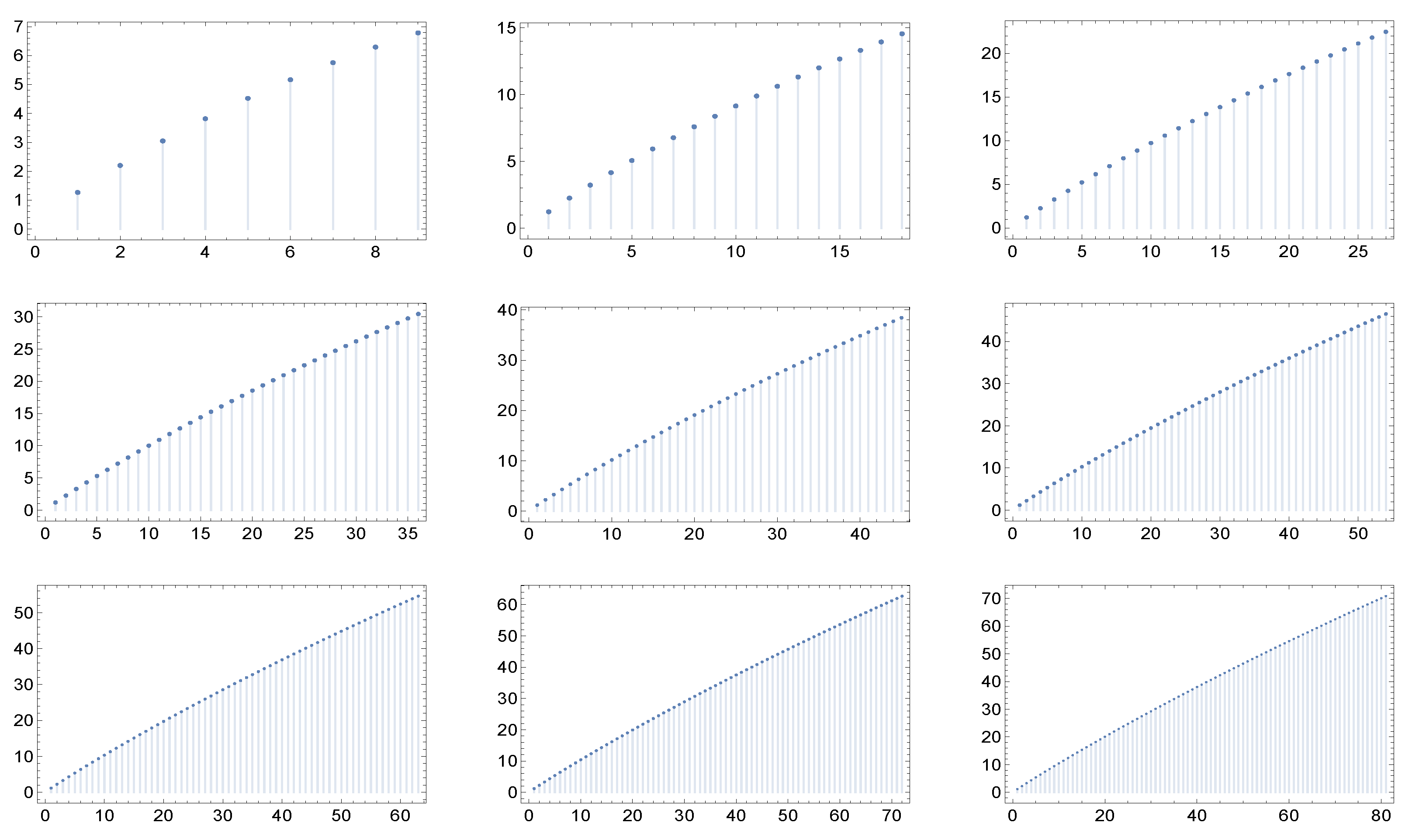
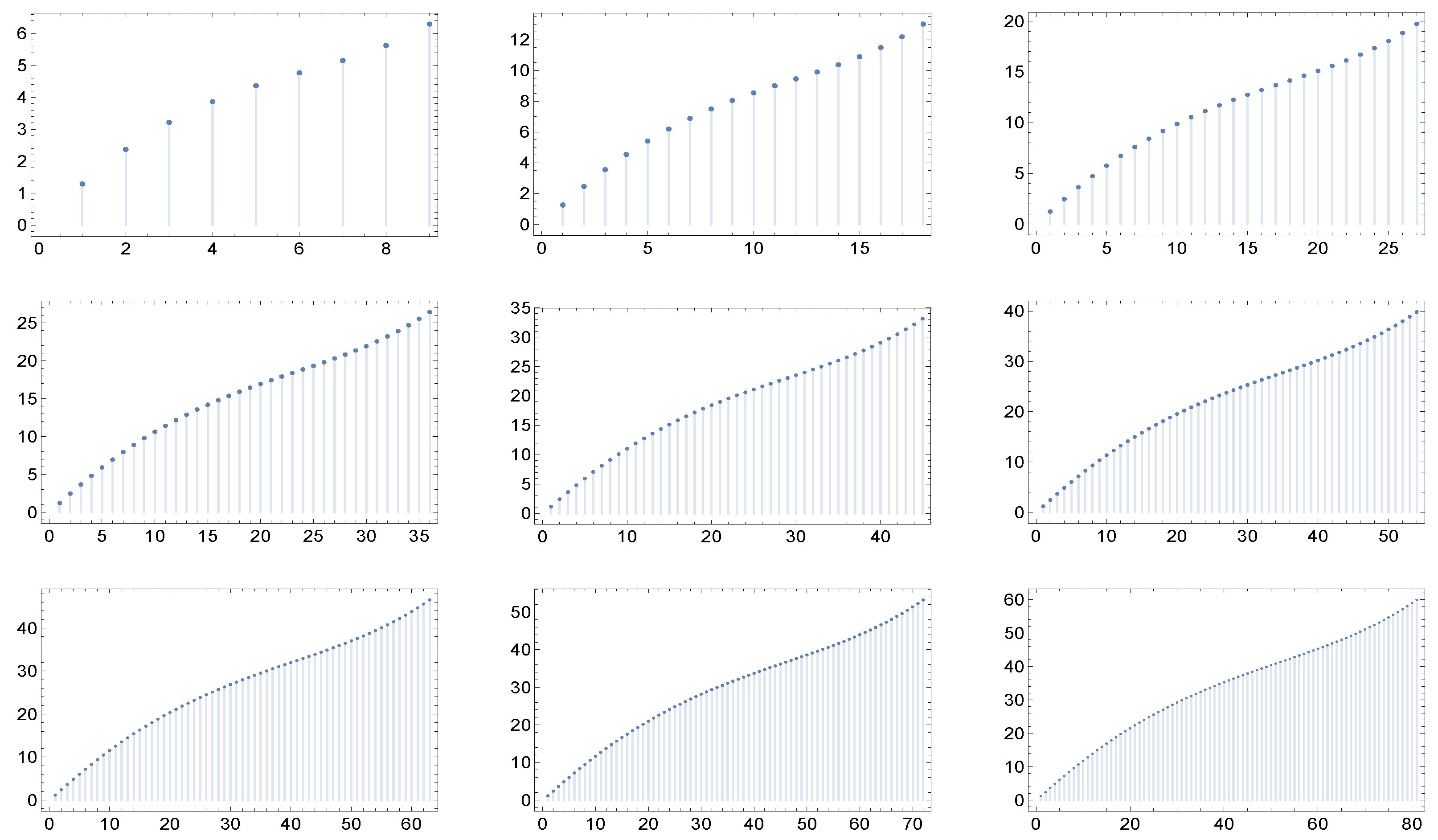
Figure 1, Figure 2, Figure 3, Figure 4, Figure 5 and Figure 6 display for each of the described network cases the graphs of the function $k_{nn}\left(k\right)$ in correspondence to nine different values of the maximum degree: 9, 18, 27, 36, 45, 54, 63, 72, and 81. Of course, we have to fix in each case a particular value of the parameters, and these are specified in the captions of the figures.

What catches the eye and is especially evident in Figure 4 and Figure 5, is that in each of the six cases the shape of the graphs of $k_{nn}\left(k\right)$ exhibit a kind of invariance with respect to the maximum degree and correspondingly, in view of the criterium of Dorogovtsev and Mendes [19], with respect to the network dimension (the number of nodes). Furthermore, the same holds true for higher values of the maximum degree.

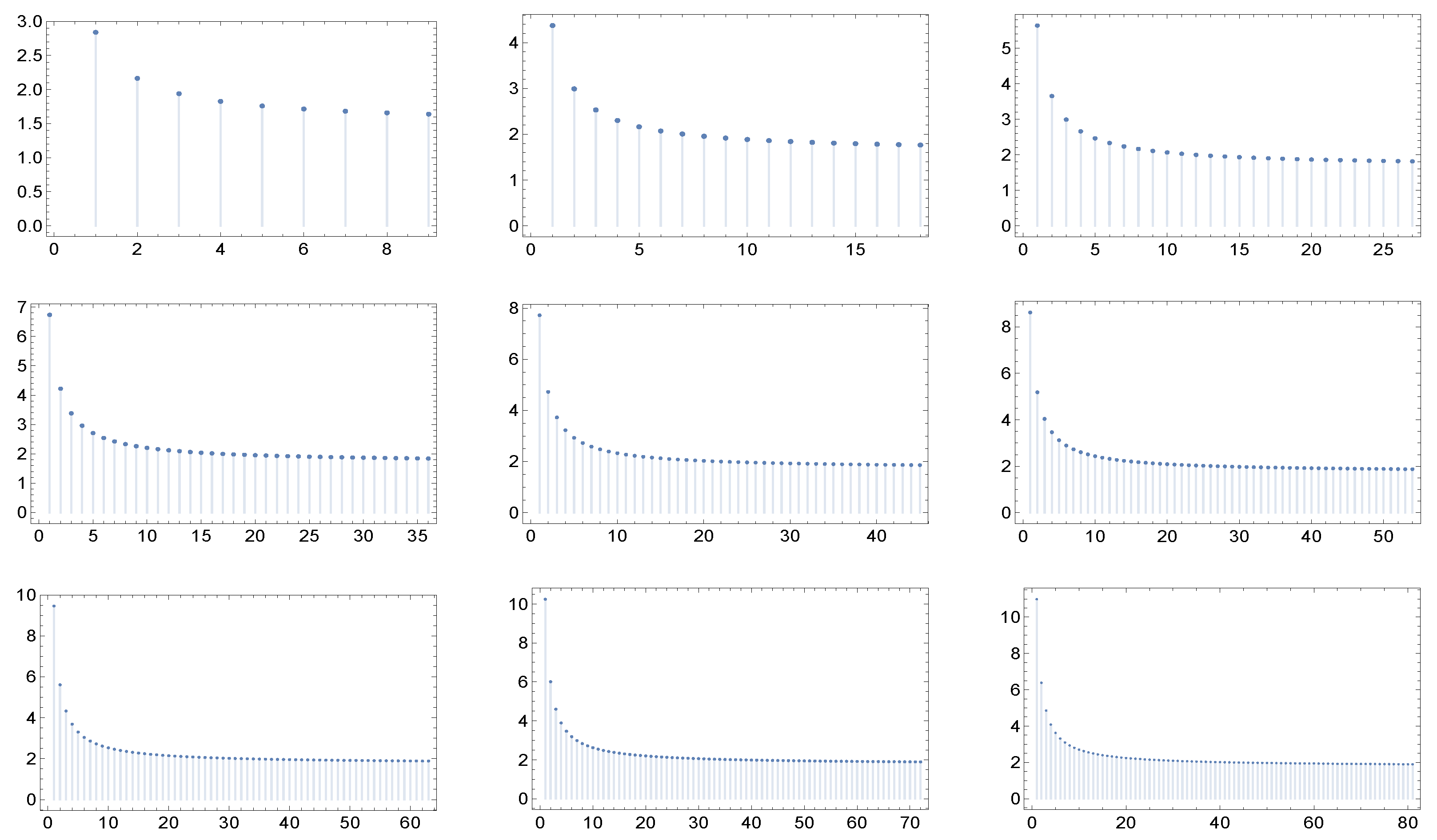
One can wonder here whether this invariant-type behavior is a consequence of the scale-free character of the degree distribution. Notice that if, for example, $P\left(k\right)\sim k^{4}exp(-k)$ (a case in which the degree distribution does not have the scale-free property) and the $P(h\mid k)$ are chosen as in $3$) above with $\lambda =1$, no invariance as in the Figure 1, Figure 2, Figure 3, Figure 4, Figure 5 and Figure 6 is found. This fact is illustrated in the Figure 7.

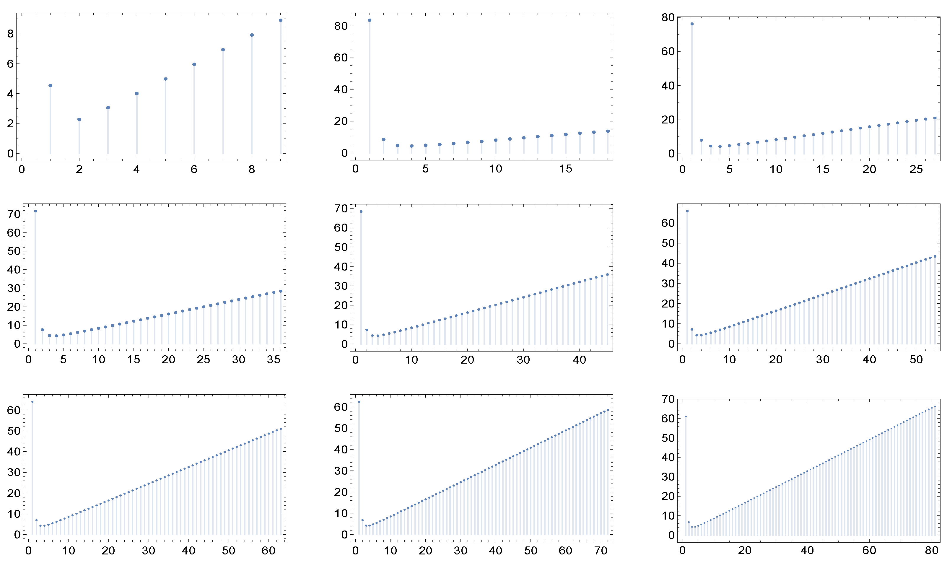
The situation is different when one constructs, employing a rewiring procedure as mentioned in the Introduction, concrete networks tentatively having a prescribed matrix $P(h\mid k)$ and then plots the averaged functions $k_{nn}\left(k\right)$ for an ensemble of them. Observing that, thanks to the formulae (5) and (6) above, such a construction can be achieved through the generation of networks having a prescribed matrix $e_{k,h}$, we here recall that an algorithm specifically aimed at this (more precisely, aimed at generating networks displaying on average a target matrix $e_{k,h}$) is described, for example, in [8]. 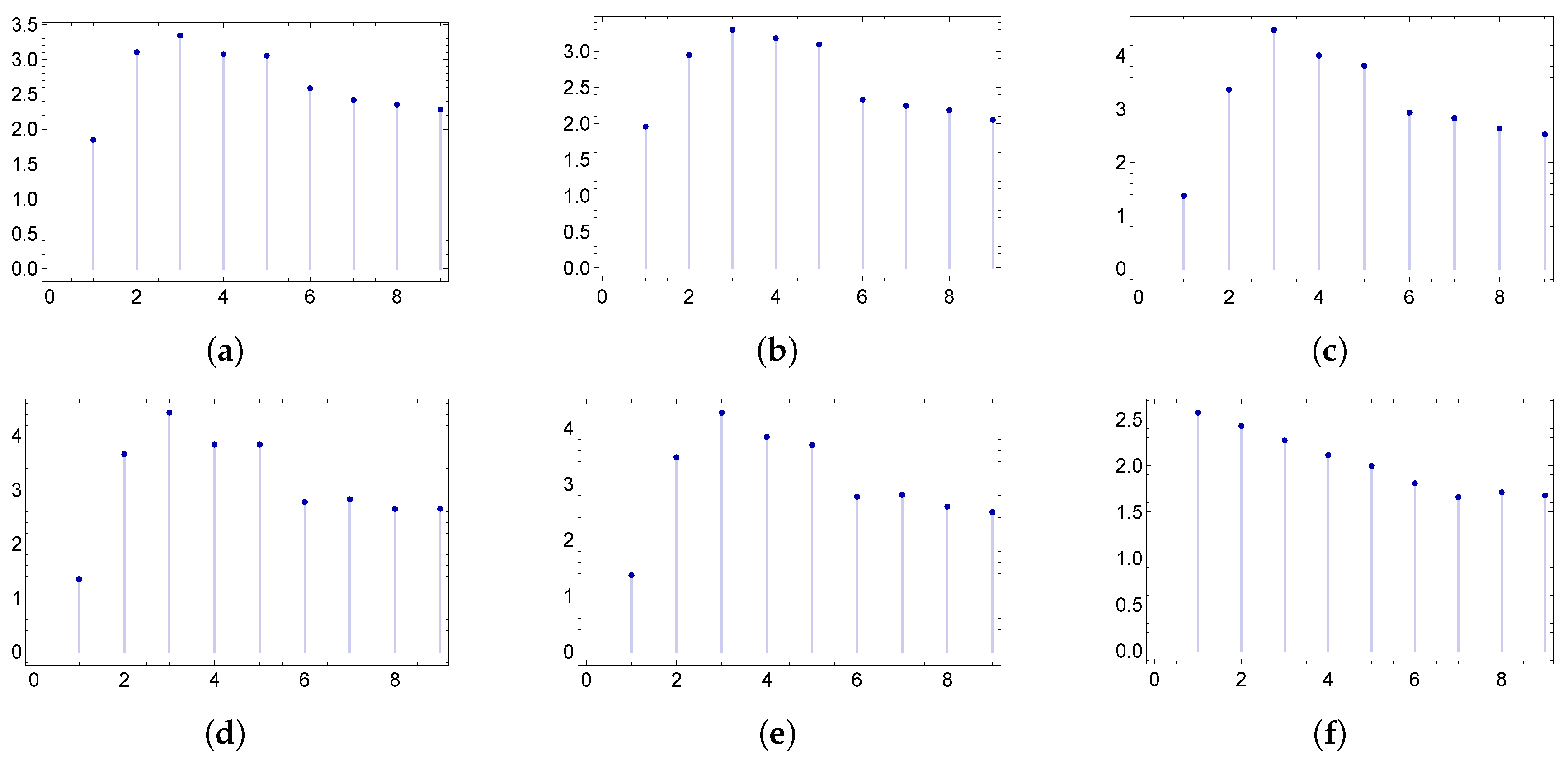We employed this algorithm to generate the networks from which we obtained, through the procedure described below, the averaged $k_{nn}\left(k\right)$ displayed in the Figure 8.

The details of the procedure we employed to generate the graphs of the $k_{nn}\left(k\right)$ displayed in the Figure 8 are described next.

We fixed the maximum degree $n=9$ and the exponent of the power-law $\gamma =2.5$. Then, for each of the six cases introduced above we carried out the following steps. We randomly took as “step zero-networks” 30 synthetic networks with degree distribution “close” to a “true” power-law distribution with these parameter values (the degree distribution of concrete scale-free assortative networks cannot display an exact power-law behavior, because in such networks only a few hubs can be present; for a discussion on the construction of a discretized degree distribution see, e.g., in [12]). On any such network we let $50.000$ steps of a (Newman) rewiring run (the number $50.000$ being suitable for a stabilization of the assortativity coefficient). We chose 30 “snapshot” networks out of the set of each rewired network more precisely, the networks obtained in correspondence of the steps $50.000-j\ast 100$ with $j=0,1,2,\cdots ,29$) and for these we constructed the matrices $e_{k,h}$. In each of the 30 cases, we then constructed a new matrix $e_{k,h}^{\left[j\right]}$ (for $j\in \{1,\cdots ,30\}$) as the average of the 30 “snapshot” matrices just obtained; through the Formula (5) we generated the correlation matrix $P^{\left[j\right]}(h\mid k)$ corresponding to this $e_{k,h}^{\left[j\right]}$ and we employed networks generated in this way as networks on top of which to study the diffusion problem described in Section 4. We also calculated the average $e_{k,h}^{\ast }$ of 30 matrices $e_{k,h}^{\left[j\right]}$ with $j\in \{1,\cdots ,30\}$ and, using (5), we generated the correlation matrix $P^{\ast }(h\mid k)$ corresponding to this $e_{k,h}^{\ast }$ as well as its associated $k_{nn}\left(k\right)$. The panels in Figure 8 clearly show that when concrete networks are constructed, even in the assortative case the function $k_{nn}\left(k\right)$ is not always increasing. This behavior, related to what is known in the literature as structural cut-off [5], is evidently due to the fact that in a network with a power-like decreasing degree distribution hubs cannot find many other hubs to which link. This finding is also compatible with the results one gets when calculating the assortativity coefficient r. The values of r for the six Markovian networks with $n=9$, $P\left(k\right)=c/k^{2.5}$, and the $P(h\mid k)$ as described at the points (1)–(6) in Section 3 are given in the first line in

Table 1. In the first line, the values of r are given for six Markovian networks as in the points (1)–(6) of Section 3 (with $P\left(k\right)=c/k^{2.5}$ and $n=9$). In the second line, for each of the cases (1)–(6), the averaged value is given of the assortativity coefficients of the networks corresponding to the thirty matrices $e_{k,h}^{\left[j\right]}$ (with $j\in \{1,\cdots ,30\}$) generated by a rewiring.

Assortativity Coefficient r	net 1	net 2	net 3	net 4	net 5	net 6
in the mean-field approach	0.20	0.50	0.75	0.67	0.61	−0.20
as an average for concrete networks	0.15	0.11	0.32	0.30	0.30	−0.13
with standard error of the mean	0.01	0.01	0.02	0.02	0.02	0.01

. In contrast, in the second line of the table one has, for each of the cases (1)–(6), the value obtained as average of the assortativity coefficients of the networks corresponding to the thirty matrices $e_{k,h}^{\left[j\right]}$ (with $j\in \{1,\cdots ,30\}$) generated by the rewiring.

4. The Peak Time in Innovation Diffusion Dynamics

In this section, we explore the effects of assortativity in different approaches within the context of an application. Specifically, we deal with the innovation diffusion process and we consider two different frameworks designed to incorporate into the classic Bass model [20] a structure of complex networks accounting for social interactions.

We start considering networks with maximum degree n, degree distribution $P\left(k\right)=c/k^{\gamma }$ where $\gamma \in (2,3)$ and c is the constant providing the normalization of P, and correlation coefficients $P(h\mid k)$ as in the six cases described in Section 3. The ratio to also consider a disassortative sample of networks is that in the innovation diffusion context also interaction and collaboration of firms can be of interest and firm networks can display disassortative mixing [16]. Recalling that the main ingredients of the process, namely, the innovation and the imitation attitude, can be quantified, respectively, through two parameters p and q, we formulate (see also in [16]) the first framework as the system of n nonlinear ordinary differential equations

$$\frac{d}{dt}{x}_j\left(t\right)=[1-x_j\left(t\right)]\left[p+jq\sum _{h=1}^{n}P(h\mid j)x_h\left(t\right)\right]\mathrm{for}j=1,\cdots ,n.$$

(15)

Each of these equations describes the variation in time of the fraction $x_j\left(t\right)$ of potential adopters (for example, individuals or firms, depending on the specific context concerned) who have j links and at the time t have adopted the innovation (In each link class the number of potential adopters is fixed.). Accordingly, the potential adopters corresponding to nodes with degree j are regarded as all “behaving” in a same way. This corresponds to a heterogeneous mean-field scenario.

A different approach consists in generating concrete networks as suggested in Section 3, writing for each network a system of evolution equations for the state of each node of the network, numerically solving the equations, calculating the peak time and taking an average out of several such times. The equation system on a concrete network can be derived by a first moment closure (see in this connection [21,22]) and takes the form

$$\frac{d}{dt}{X}_i\left(t\right)=(1-X_i\left(t\right))\left[p+q\sum _{j=1}^N{A}_{ij}{X}_j\left(t\right)\right]\mathrm{for}i=1,\cdots ,N,$$

(16)

where N and $A_{ij}$ respectively denote the number of network nodes and the elements of the adjacency matrix. The variable $X_i$ with $i=1,\cdots ,N$ has to be understood as the expectation $\langle {\xi }_i\rangle$ of the non-adoption (${\xi }_i=0$) or adoption (${\xi }_i=1$) state of node i over many stochastic evolutions of the system.

An important time in the diffusion process of an innovation is the so-called peak time which is the moment when the adoption rate assumes its maximum value. In connection with the six cases defined in Section 3, we calculated the peak time both in a mean-field approach and for an ensemble of concrete networks, constructed through the procedure outlined in the same section.

To carry out the numerical simulations, we chose $p=p^{\ast }$ and $q=q^{\ast }/M$, where the parameters $p^{\ast }=0.03$ and $q^{\ast }=0.4$ are as in the original Bass paper [20], and the constant $M={\displaystyle \sum _{h=1}^n}hP\left(h\right)$ provides a proper adjustment for the imitation coefficient on networks. Furthermore, we fixed $n=9$ and $\gamma =2.5$. 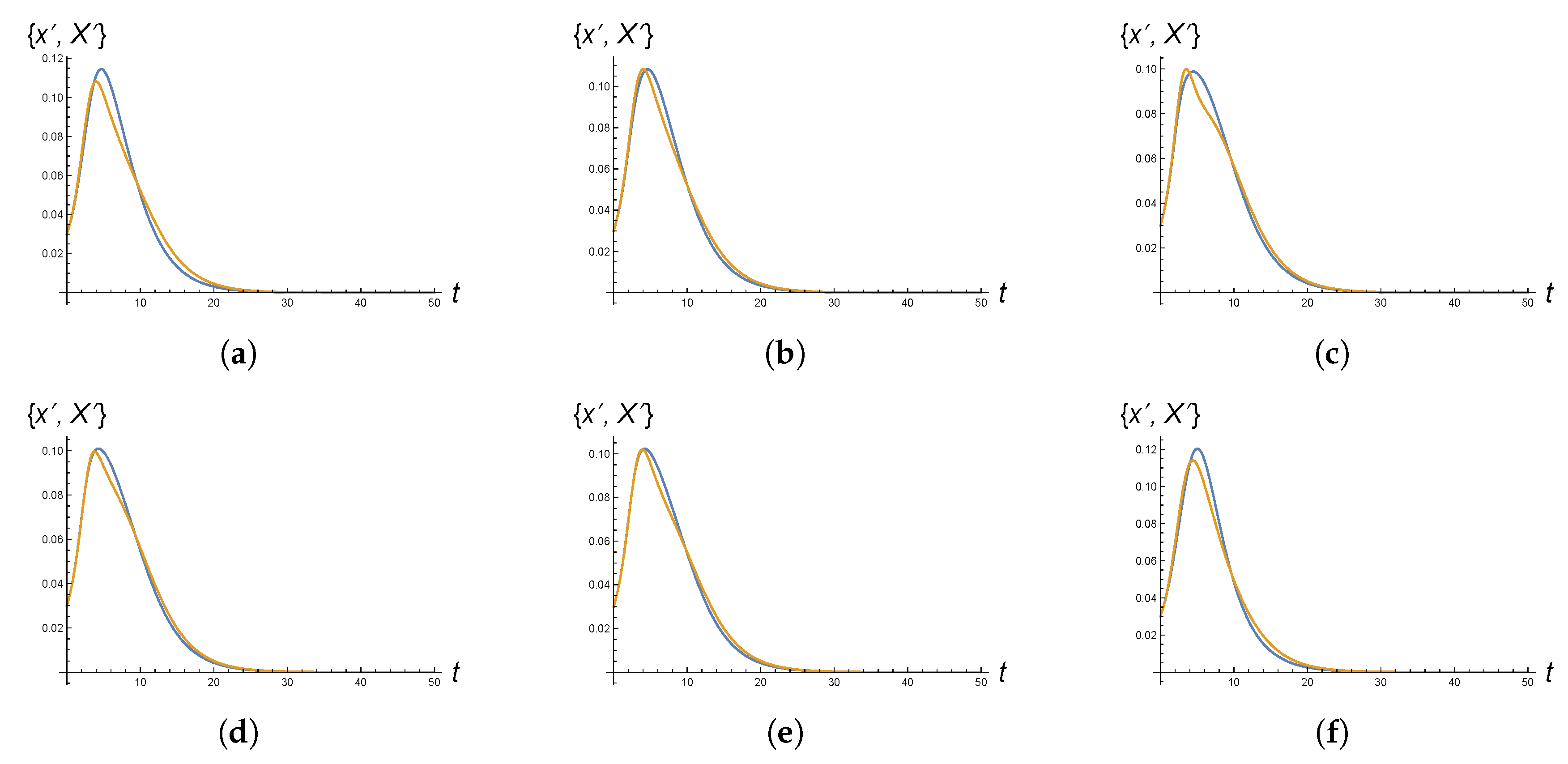For each of the six Markovian networks with correlation matrices described in the points (1)–(6) of Section 3, we computed numerical solutions of the Equation (15). Then, we also performed the second procedure described above, which involves numerically solving an ensemble of equation systems (16). With regard to this approach, we took in each case (1)–(6) the average peak time out of a set of peak times relative to 30 networks. The values we found are reported in the

Table 2. The values are here reported of the peak time for six networks with correlation matrices as in the points (1)–(6) of Section 3. The values in the first line are evaluated within a mean-field approach, those in the second line are obtained as averages of peak times over concrete networks.

Peak Time Evaluated	net 1	net 2	net 3	net 4	net 5	net 6
in the mean-field approach	4.68	4.61	4.45	4.30	4.23	5.03
as an average for concrete networks	4.28	4.28	3.94	3.93	4.00	4.68
with standard error of the mean	0.04	0.03	0.04	0.04	0.03	0.03

. There are of course differences between the peak times obtained through one and the other approach, but qualitatively one finds rather similar results. In particular, for almost each pair of networks the ordering relation between the values of their peak time as computed via one and the other approach is the same. Moreover, when looking at the plots, see, e.g., Figure 9, which display the time evolution of the functions $x^{\prime }\left(t\right)={\sum }_{j=1}^n\frac{d}{dt}{x}_j\left(t\right)$ and $X^{\prime }={\sum }_{i=1}^N\frac{d}{dt}{X}_i\left(t\right)$, derivatives of the “cumulative” solutions of the systems (15) and (16), respectively, one notices a reasonable agreement.

5. Further Remarks on the Function ${\mathit{k}}_{\mathit{nn}}$ and Its Average

As is also apparent from Section 3, the range of correlation matrix families is rather wide, and the functions $k_{nn}$ corresponding to these families can be quite different from each other.

In this regard, we observe that in [6,7], which deal with epidemic spreading in complex networks and, in particular, with the existence or non-existence of an epidemic threshold, an average of the average nearest neighbor degree function $k_{nn}\left(k\right)$,

$$K_n=\sum _{k=1}^{n}P\left(k\right)k_{nn}\left(k\right),$$

(17)

is also introduced, whose properties are then explored (In [6] and [7] a different notation from that one adopted here is used to indicate the average in (17)). Notably, in the assortative case, the ansatz is there considered that $k_{nn}\left(k\right)\propto k^{\beta }$ for some positive $\beta$. It is then shown that $K_n$ tends to infinity as $n\to \infty$. This property does not seem to be satisfied in general, namely, for all assortative families, by the relative $K_n$. 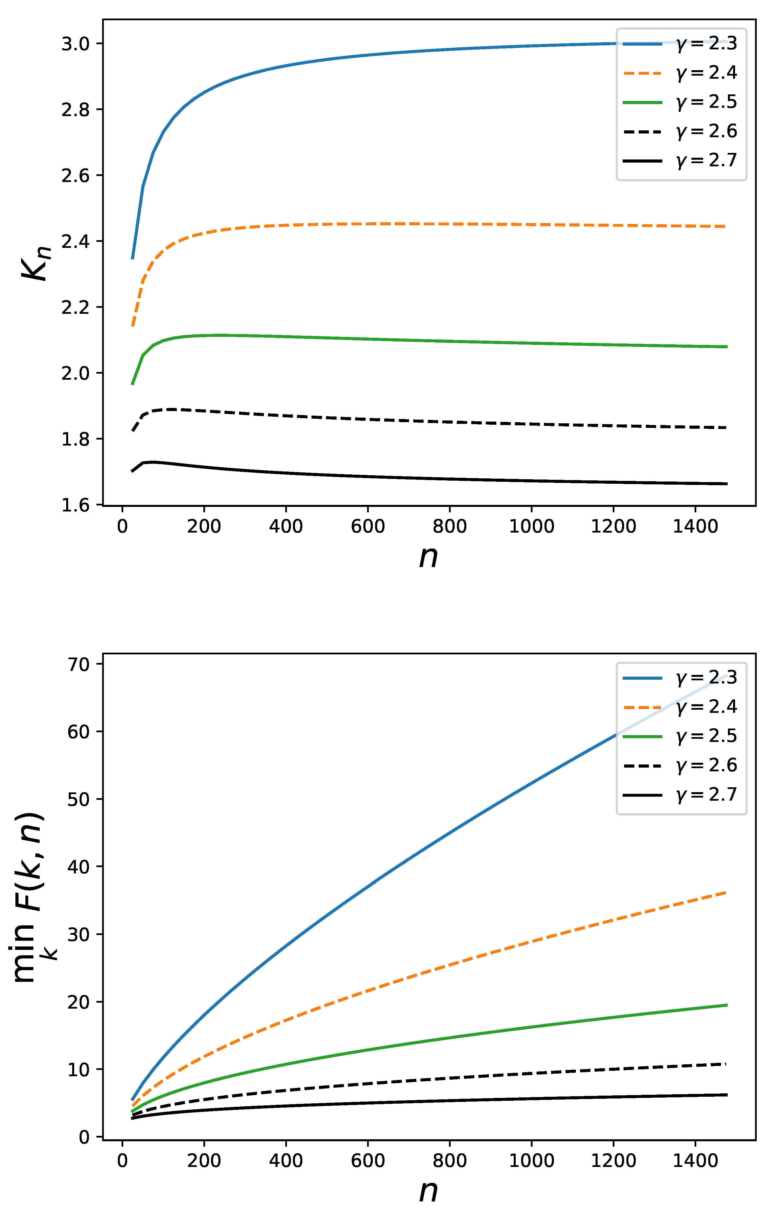For instance, for the exponential family $\left(5\right)$ of Section 3 one can numerically check that the dependence of $K_n$ on n in correspondence to various values of the exponent $\gamma$ occurring in the degree distribution is as displayed in the left panel of the Figure 10. At least for certain values of $\gamma$ the value of $K_n$ is not increasing and does not look at all as tending to infinity as $n\to \infty$. However, of course, as well shown in Figure 5, the function $k_{nn}\left(k\right)$ for the exponential family $\left(5\right)$ does not grow as $k^{\beta }$. It has nonetheless to be emphasized that also for this family the crucial property towards the determination of the absence of epidemic threshold [6,7], namely the growing character of

$$\underset{k}{min}F(n,k)=\underset{k}{min}\sum _{h=1}^{n}hP(h\mid k)k_{nn}\left(h\right)$$

(18)

as a function of n is satisfied, see the right panel of Figure 10.

In connection with the innovation diffusion problem, one may wonder whether some correlation exists between the values of $K_n$ and the peak times. Let us take for example networks with degree distribution $P\left(k\right)\propto 1/k^{\gamma }$ whose correlation matrices $P(h\mid k)$ are as in $\left(5\right)$ of Section 3 with $\nu =1$ and consider nine values of the scale-free exponent $\gamma$, i.e., $\gamma =2+\left(0.1\right)j$ for $j=1,\cdots 9$ (In this way, we are fixing the correlations and varying the degree distribution).

From

Table 3. These three tables display values of $K_n$ and of the peak times $t_{max}$ in correspondence of different values of the parameters $\gamma$ for networks with $P\left(k\right)\propto 1/k^{\gamma }$ and correlation matrices as in $\left(5\right)$ of Section 3 with $\nu =1$. The tables are relative, respectively, to $n=9$ (table on the left), $n=45$ (central table), and $n=81$ (table on the right).

$\mathit{\gamma }$	${\mathit{K}}_{\mathit{n}}$	${\mathit{t}}_{\mathit{max}}$
n = 9
2.1	2.20	4.00
2.2	2.07	4.02
2.3	1.96	4.06
2.4	1.85	4.14
2.5	1.75	4.22
2.6	1.67	4.36
2.7	1.60	4.50
2.8	1.53	4.64
2.9	1.47	4.80
n = 45
2.1	3.30	2.00
2.2	2.88	2.32
2.3	2.54	3.08
2.4	2.26	3.76
2.5	2.04	4.24
2.6	1.87	4.58
2.7	1.73	4.84
2.8	1.61	5.02
2.9	1.52	5.18
n = 81
2.1	3.70	1.48
2.2	3.12	2.48
2.3	2.69	3.54
2.4	2.35	4.16
2.5	2.09	4.54
2.6	1.89	4.82
2.7	1.73	5.04
2.8	1.61	5.18
2.9	1.51	5.30

, we see that at fixed n, the values of $K_n$ and $t_{max}$ display a quite strong dependence on $\gamma$, namely, $K_n$ is decreasing in $\gamma$, while $t_{max}$ is increasing. We note in this regard that the implicit relation between $K_n$ and $t_{max}$ is quite in agreement with intuition, because diffusion is expected to be faster when each node has, on the average, neighbors of higher degree. Varying the maximum degree n, we see that the dependence of $K_n$ and $t_{max}$ on $\gamma$ becomes stronger as n grows.

It is also possible to test the dependence of $K_n$ and $t_{max}$ on the correlations, for instance, by varying the parameter $\nu$. The resulting dependence is generally weak and details depend on n. For instance, in

Table 4. These two tables display values of the peak times $t_{max}$ in correspondence of different values of the parameters $\gamma$ and $\nu$ for networks with $P\left(k\right)\propto 1/k^{\gamma }$ and correlation matrices as in $\left(5\right)$ of Section 3. The table above is relative to $n=9$, the table below is relative to $n=81$.

${\mathit{t}}_{\mathit{max}}$	$\mathit{\nu }=0.2$	$\mathit{\nu }=0.4$	$\mathit{\nu }=0.6$	$\mathit{\nu }=0.8$	$\mathit{\nu }=1$
n = 9
$\gamma =2.1$	4.04	4.04	4.02	4.02	4.00
$\gamma =2.2$	4.04	4.04	4.04	4.04	4.02
$\gamma =2.3$	4.06	4.06	4.08	4.06	4.06
$\gamma =2.4$	4.12	4.12	4.12	4.14	4.14
$\gamma =2.5$	4.20	4.20	4.22	4.22	4.22
$\gamma =2.6$	4.30	4.32	4.32	4.34	4.36
$\gamma =2.7$	4.44	4.44	4.46	4.48	4.50
$\gamma =2.8$	4.58	4.60	4.62	4.62	4.64
$\gamma =2.9$	4.74	4.76	4.76	4.78	4.80
n = 81
$\gamma =2.1$	1.38	1.40	1.42	1.46	1.48
$\gamma =2.2$	2.26	2.32	2.36	2.42	2.48
$\gamma =2.3$	3.56	3.54	3.54	3.54	3.54
$\gamma =2.4$	4.18	4.16	4.16	4.16	4.16
$\gamma =2.5$	4.58	4.56	4.56	4.56	4.54
$\gamma =2.6$	4.86	4.84	4.84	4.84	4.82
$\gamma =2.7$	5.06	5.04	5.04	5.04	5.04
$\gamma =2.8$	5.20	5.20	5.20	5.18	5.18
$\gamma =2.9$	5.32	5.32	5.30	5.30	5.30

we report the dependence of $t_{max}$ on $\gamma$ and $\nu$ (considering $\nu =\left(0.2\right)j$ for $j=1,\cdots 5$) for the cases $n=9$ and $n=81$. It can be seen that for $n=9$ the values of $t_{max}$ decrease slightly in $\nu$ at small $\gamma$ and increase slightly in $\nu$ at large $\gamma$, while for $n=81$ the opposite is true.

En passant, we mention here that the correlation between $K_n$ and r has been investigated from another perspective (namely, along a network rewiring process) in [23].

Last, two more general properties involving the function $k_{nn}$ are worth being noticed.

- A normalization property [6,7]: One has (here and henceforth $\langle f\left(k\right)\rangle$ denotes ${\sum }_{k=1}^{n}f\left(k\right)P\left(k\right)$.)

$$\sum _{k=1}^{n}kP\left(k\right)k_{nn}\left(k\right)=\langle k^2\rangle .$$

(19)

The formula (19) can be useful for calculating the constant c appearing in an ansatz as $k_{nn}\left(k\right)=c{k}^{\beta }$. One finds indeed $c=\langle k^2\rangle /\langle k^{\beta +1}\rangle$.

Proof. 

of (19): The normalization property (19) immediately follows from the Network Closure Condition (3): one multiplies by h the left and the right hand side of (3), and then takes on both sides the sums for h and k from 1 to n to get $\langle k^2\rangle$ on the l.h.s in view of (2) and ${\sum }_{k=1}^{n}kP\left(k\right)k_{nn}\left(k\right)$ on the r.h.s in view of the expression (1) of $k_{nn}\left(k\right)$. □

- Relation with the correlation coefficient: One has

$$r=\frac{\langle k\rangle {\sum }_{k=1}^n{k}^{2}P\left(k\right)k_{nn}\left(k\right)-{\langle k^2\rangle }^2}{\langle k\rangle \langle k^3\rangle -{\langle k^2\rangle }^2}.$$

(20)

The formula (20) can be employed for example for calculating r when the function $k_{nn}$ is determined by the ansatz $k_{nn}\left(k\right)=c{k}^{\beta }$. In such a case one does not need to know the correlation coefficients: only the expression of $k_{nn}$ and of some averages depending on the degree distribution appear on the r.h.s. of (20).

Proof. 

of (20): We consider separately the terms appearing in the expression of the correlation coefficient r in (4). □

Let us start with the first term in the numerator on the r.h.s of (4). Recalling that

$$e_{hk}={\tilde{e}}_{h+1,k+1}\mathrm{and}{\tilde{e}}_{hk}=\frac{1}{k_m}P(h\mid k)kP\left(k\right),$$

we can write

$$\sum _{h,k=0}^{n-1}hk{e}_{hk}=\sum _{h^{\prime },k^{\prime }=1}^n\frac{1}{k_m}(h^{\prime }-1)(k^{\prime }-1)P(h^{\prime }\mid k^{\prime })k^{\prime }P\left(k^{\prime }\right),$$

(21)

where $h^{\prime }=h+1$, $k^{\prime }=k+1$ and $k_m=\langle k\rangle$.

Renaming for simplicity h and k the indices, we now transform the four terms which can be obtained on the r.h.s. of (21) when the product is expanded to get

(i)

$\frac{1}{k_m}{\sum }_{h,k}hkP(h\mid k)kP\left(k\right)$,

(ii)

$-\frac{1}{k_m}{\sum }_{h,k}hP(h\mid k)kP\left(k\right)$,

(iii)

$-\frac{1}{k_m}{\sum }_{h,k}kP(h\mid k)kP\left(k\right)$,

(iv)

$\frac{1}{k_m}{\sum }_{h,k}P(h\mid k)kP\left(k\right)$.

By exploiting in these expressions the Formules (1) and (2) and also using (19), we rewrite these terms, respectively, as

(i)

$\frac{1}{k_m}{\sum }_k{k}^{2}P\left(k\right)k_{nn}\left(k\right)$,

(ii)

$-\frac{1}{k_m}\langle k^2\rangle$,

(iii)

$-\frac{1}{k_m}\langle k^2\rangle$,

(iv)

$\frac{k_m}{k_m}$.

Summarizing, we get

$$\sum _{h,k=0}^{n-1}hk{e}_{hk}=\frac{1}{k_m}\left(\sum _{k=1}^n{k}^{2}P\left(k\right)k_{nn}\left(k\right)-2\langle k^2\rangle +k_m\right).$$

The second term in the numerator is ${\sum }_{h,k=0}^{n-1}hk(-q_h{q}_k)$. Recalling that $q_k=\frac{(k+1)P(k+1)}{k_m}$, we rewrite it as

$$-\frac{1}{k_m^2}\sum _{h,k=0}^{n-1}hk(h+1)(k+1)P(h+1)P(k+1)$$

and then, by setting as above $h^{\prime }=h+1$ and $k^{\prime }=k+1$, as

$$-\frac{1}{k_m^2}\sum _{h^{\prime },k^{\prime }=1}^n(h^{\prime }-1)(k^{\prime }-1)h^{\prime }{k}^{\prime }P\left(h^{\prime }\right)P\left(k^{\prime }\right).$$

with renamed indices this becomes

$$-\frac{1}{k_m^2}\sum _{h,k=1}^n(hk-h-k+1)hkP\left(h\right)P\left(k\right)=\dots =-\frac{1}{k_m^2}\left(\langle k^2\rangle \langle k^2\rangle -2\langle k^2\rangle k_m+k_m^2\right).$$

The numerator on the r.h.s. of (4) is thus

$$\sum _{h,k=0}^{n-1}hk\left(e_{hk}-q_h{q}_k\right)=\frac{1}{k_m}\sum _{k=1}^n{k}^{2}P\left(k\right)k_{nn}\left(k\right)-\frac{1}{k_m^2}{\langle k^2\rangle }^2.$$

The denominator on the r.h.s. of (4) only contains quantities which depend on the $q_k$, and correspondingly on the degree distribution, and not on the correlation coefficients. These quantities can be expressed in terms of the moments $\langle k\rangle$, $\langle k^2\rangle$ e $\langle k^3\rangle$ as follows.

$$\sum _{k=0}^{n-1}{k}^2{q}_k=\sum _{k=0}^{n-1}{k}^2\frac{1}{k_m}(k+1)P(k+1)=\sum _{k^{\prime }=1}^n{(k^{\prime }-1)}^2\frac{1}{k_m}{k}^{\prime }P\left(k^{\prime }\right)=\dots =\frac{1}{k_m}\left(\langle k^3\rangle -2\langle k^2\rangle +\langle k\rangle \right)$$

and

$${\left(\sum _{k=0}^{n-1}k{q}_k\right)}^2={\left(\sum _{k=0}^{n-1}k\frac{1}{k_m}(k+1)P(k+1)\right)}^2=\frac{1}{k_m^2}{\left(\sum _{k^{\prime }=1}^n(k^{\prime }-1)k^{\prime }P\left(k^{\prime }\right)\right)}^2=\frac{1}{k_m^2}{\left(\langle k^2\rangle -\langle k\rangle \right)}^2.$$

In conclusion, the denominator on the r.h.s. of (4) is

$$\frac{1}{\langle k\rangle }\left(\langle k^3\rangle -2\langle k^2\rangle +\langle k\rangle \right)-\frac{1}{{\langle k\rangle }^2}{\left(\langle k^2\rangle -\langle k\rangle \right)}^2=\frac{\langle k^3\rangle }{\langle k\rangle }-{\left(\frac{\langle k^2\rangle }{\langle k\rangle }\right)}^2$$

and

$$r=\frac{\frac{1}{\langle k\rangle }{\sum }_{k=1}^n{k}^{2}P\left(k\right)k_{nn}\left(k\right)-{\left(\frac{\langle k^2\rangle }{\langle k\rangle }\right)}^2}{\frac{\langle k^3\rangle }{\langle k\rangle }-{\left(\frac{\langle k^2\rangle }{\langle k\rangle }\right)}^2}=\frac{\langle k\rangle {\sum }_{k=1}^n{k}^{2}P\left(k\right)k_{nn}\left(k\right)-{\langle k^2\rangle }^2}{\langle k\rangle \langle k^3\rangle -{\langle k^2\rangle }^2}.$$

6. Conclusions

This paper took shape from the investigation, carried out through two different mathematical frameworks, of some dynamical systems on top of synthetic correlated networks. Beside the description of the two approaches and of some findings obtained with them, the paper contains comments and observations on various features emerged. We emphasize next the main facets found as output of several numerical simulations.

– A singular and unexpected property is revealed for the six families of scale-free Markovian networks (characterized by given correlation coefficients) considered here: the graphs of the average nearest neighbor degree function $k_{nn}\left(k\right)$, usually employed to detect assortativity or disassortativity, display an apparently ignored quasi-invariance with respect to the maximal degree of the network and, accordingly, its dimension. In our view, this is an interesting aspect, which deserves deeper inspection and understanding.

– The existence of correlated networks is shown whose average nearest neighbor degree function $k_{nn}\left(k\right)$ does not behave as $\alpha k^{\beta }$ with some coefficient $\alpha$ and $\beta$. See indeed, e.g., the graphs in Figure 4 and Figure 5. In general, in the literature, the functions $k_{nn}\left(k\right)$ analytically expressed by means of the correlation coefficients are supposed to behave as $\alpha k^{\beta }$, see, e.g., in [5,6,7,17,18,24]. Only after writing this paper, did we learn from one of its referees of the existence of a recent work, [25], where a $k_{nn}\left(k\right)$ is constructed, which does not behave as $\alpha k^{\beta }$.

– Unavoidable differences are found and illustrated between the graphs of the function $k_{nn}\left(k\right)$ in the case of Markovian scale-free networks and of concrete assortative scale-free networks. See also, in this connection, the discussion on the conflict between degree correlations and the scale-free property in [5]. Independently of this, we can conclude that, at least with reference to the diffusion problem explored in Section 4, the mean-field approach provides quite satisfactory results. Furthermore, of course, it has the advantage of being much less demanding from the computational point of view, in particular when larger networks are involved.

We notice that a functional behavior in k as in the ansatz $k_{nn}\left(k\right)=\alpha k^{\beta }$ is intrinsically independent from any scale. In the presence of such an anstatz it is therefore inevitable that the graph of $k_{nn}\left(k\right)$ is self-similar $\left(1\right)$ for any value of the maximum degree and $\left(2\right)$ for networks having any degree distribution. The introduction of possible functional forms of $k_{nn}\left(k\right)$ as proposed in this paper allows to distinguish between the situations $\left(1\right)$ and $\left(2\right)$ above, which appear otherwise like coincident or degenerate as far as the degree distribution and degree correlations are concerned. In fact the new functions obtained for $k_{nn}\left(k\right)$ (for which there is no closed algebraic expression; they are the result of a construction procedure on the $P(h\mid k)$ performed in several steps and involving the $P\left(k\right)$) display in their plots some inflection points whose position may in general depend on the degree distribution and on n. We can therefore change separately $\left(1\right)$ the maximum degree and $\left(2\right)$ the degree distribution (from being scale-free to non scale-free) and check if these inflection points change their relative position. It turns out that, as seen in Figure 7,

$\left(a\right)$ at fixed scale-free degree distribution, the plot of $k_{nn}\left(k\right)$ is self-similar, independently from n (no change in the relative position of the inflection points);

$\left(b\right)$ at fixed non scale-free distribution, the plot is not self-similar if we change n; and

$\left(c\right)$ at fixed n, the plot is not self-similar, if we switch from scale-free to non scale-free distributions.

Again, we stress that these different behaviors cannot be observed using an ansatz for $k_{nn}\left(k\right)$ that is inherently self-similar.

It seems to us that there are few works dealing with the problem tackled here. Yet, we can mention that various mean-field approximation schemes (node-based, degree-based, pair approximation, and approximate master equation) are compared with each other in connection with applications to epidemic spreading in [22], and mean-field predictions and numerical simulation results are compared for dynamical processes running on 21 real-world networks in [26]. It is impossible to give a concise description of the various specific results contained in these two references, but we emphasize here that also their authors provide evidence of cases in which the mean-field theory works quite well. Instead, it can be worthwhile to dwell on the paper [24], where a comparison is made between mean-field predictions and simulations on large synthetic networks built with the Porto–Weber method, for some cases in which there is no decreasing tail of the $k_{nn}$ at large k. This shows that the question is still open of whether mean-field predictions also are compatible with numerical solutions on synthetic assortative networks that do display a decreasing tail, like in the real case. Our paper describes an effort in this direction. Technically, our strategy has been to $\left(1\right)$ generate “ideal” assortative correlation matrices $P(h\mid k)$ of various kinds; $\left(2\right)$ compute diffusion times of the Bass model for each $P(h\mid k)$ in the mean-field approximation; $\left(3\right)$ generate, by rewiring, synthetic scale-free networks whose real $P(h\mid k)$ is as close as possible to the given ideal $P(h\mid k)$, according to the probability method by Newman (since the procedure is quite complex and involves an intermediate averaging, see Section 3, it was limited to small n); and $\left(4\right)$ compute again diffusion times using the adjacency matrices of the synthetic networks and compare them with those of Point $\left(2\right)$. What we found is that, unlike in [24], the effective $k_{nn}\left(k\right)$ of the networks so constructed does display a decreasing tail, like in real networks. Nevertheless, the diffusion times are in reasonable agreement.

Finally, a maximal degree equal to 9, as here prevalently considered, may look quite small. The majority of papers studying complex networks deal with much greater numbers. We believe, however, that for the purpose of this paper, and to show the outlined facets and differences, this choice is sufficient and suited.