Stuck Knots

Abstract

Singular knots and links have projections involving some usual crossings and some four-valent rigid vertices. Such vertices are symmetric in the sense that no strand overpasses the other. In this research we introduce stuck knots and links to represent physical knots and links with projections involving some stuck crossings, where the physical strands get stuck together showing which strand overpasses the other at a stuck crossing. We introduce the basic elements of the theory and we give some isotopy invariants of such knots including invariants which capture the chirality (mirror imaging) of such objects. We also introduce another natural class of stuck knots, which we call relatively stuck knots, where each stuck crossing has a stuckness factor that indicates to the value of stuckness at that crossing. Amazingly, a generalized version of Jones polynomial makes an invariant of such quantized knots and links. We give applications of stuck knots and links and their invariants in modeling and understanding bonded RNA foldings, and we explore the topology of such objects with invariants involving multiplicities at the bonds. Other perspectives are also discussed.

1. Introduction

In this paper we introduce what can be thought of as a generalization of singular knots to what we call stuck knots. Diagrammatically speaking, stuck knots are singular knots or links with extra information at their vertices coming from the visual picture of two physical strands getting stuck together. When two physical strands get stuck together making a vertex, we can mostly tell which of them is over the other.

At the beginning of this paper we caution readers familiar with the physical knot theory literature that the stuck knots which are the subject of this paper are not related to the stuck unknots introduced in [1].

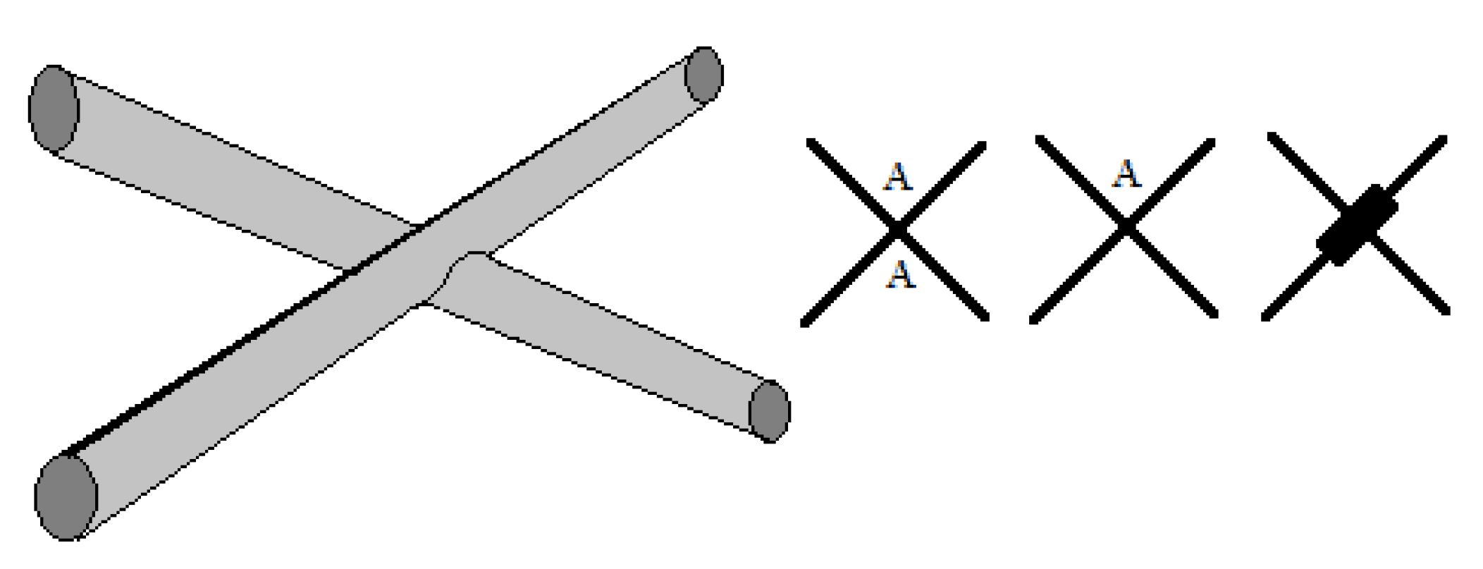
A stuck knot diagram is a knot or link diagram, which has two types of crossings; usual crossings and stuck crossings. The stuck crossings are vertices which behave like the rigid vertices in singular knots, but with a convention of which strand passes over the other. The information of which strand is stuck over the other will be represented by assigning the A-regions used by Kauffman in [2] at usual crossings. The A-regions at a stuck crossing are determined by which two opposite regions are swiped first when the upper strand rotates counter-clockwise. Since these two regions are always opposite, marking one of them will be enough to know both of them, and hence to know which strand is stuck over the other. Another way to distinguish the upper strand is by drawing a small thick line segment on the upper strand. See Figure 1 for a physical view of a stuck crossing and its diagrammatic representations.

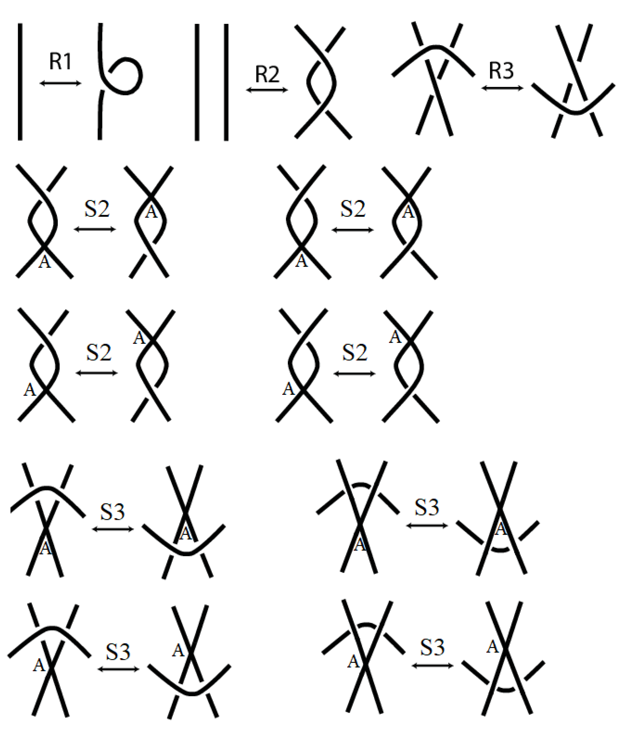
Two stuck knot diagrams are said to be isotopic if we can get each of them from the other by a finite number of the following Reidemeister-like moves. See Figure 2.

Note that if we ignore the A-regions, then these moves are similar to the moves governing the isotopy of singular knots given by Kauffman in [3]. For more on singular knots and their invariants see [4,5,6].

A stuck knot is the equivalence class of stuck not diagrams subject to the Reidemeister-like moves given above. We usually do not distinguish between a knot diagram and the class it represents. The same habit will be applied to stuck knots. An oriented stuck knot is a stuck knot provided with an orientation. Oriented stuck knots are considered subject to the oriented versions of the Reidemeister-like moves given above. Unlike oriented singular crossings, oriented stuck crossings come with a sign of $+1$ or $-1$ according to the right hand rule, because we know which strand passes over the other at a stuck crossing. Using the A-region notation, the stuck crossing will have a sign of $+1$ if the A-regions lie between the two strands with both arrows heading into or out of the stuck crossing. Otherwise the stuck crossing under consideration has a sign of $-1$.

Some immediate invariants of stuck knots or links can be defined. We define the sticking number of a stuck knot or link to be the number of stuck crossings, and the signed sticking number of an oriented stuck knot or link to be the sum of signs of the stuck crossings. For a non-oriented stuck knot (one component link), the signed sticking number can also be defined by the sum of signs of the stuck crossings obtained by any of the two possible orientations of the knot.

For an oriented two component stuck link we define the linking sticking number to be the sum of signs of the stuck crossings between the two components.

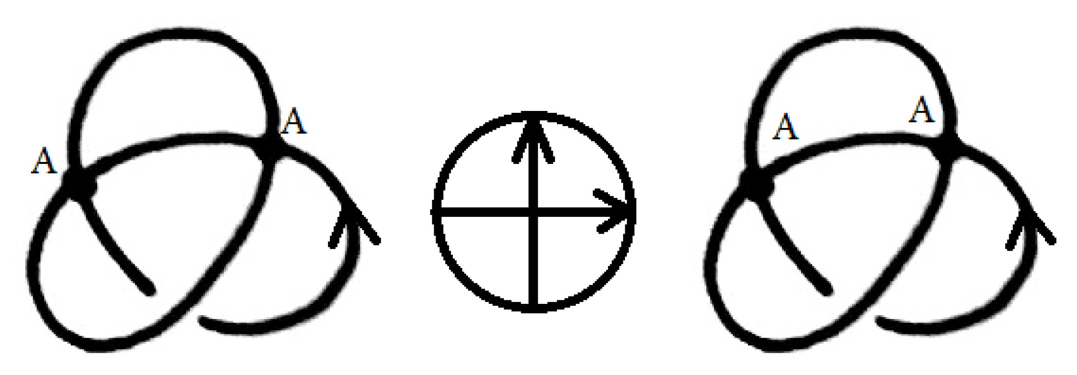
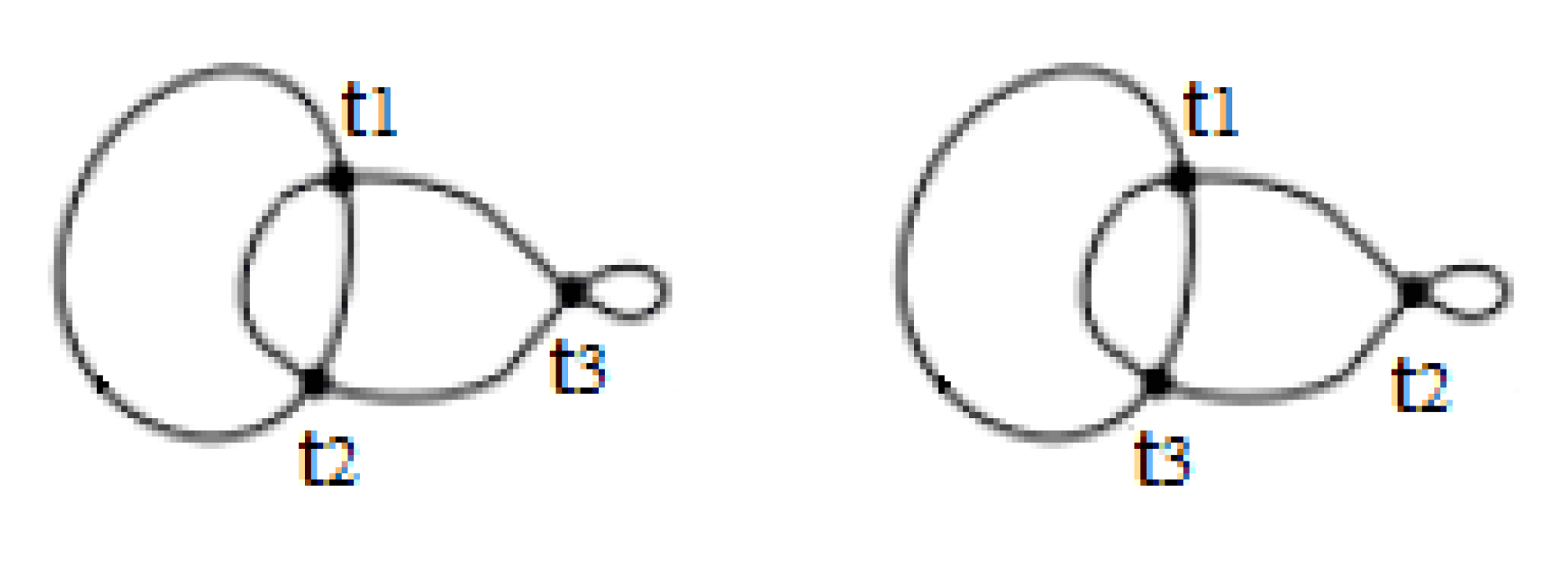
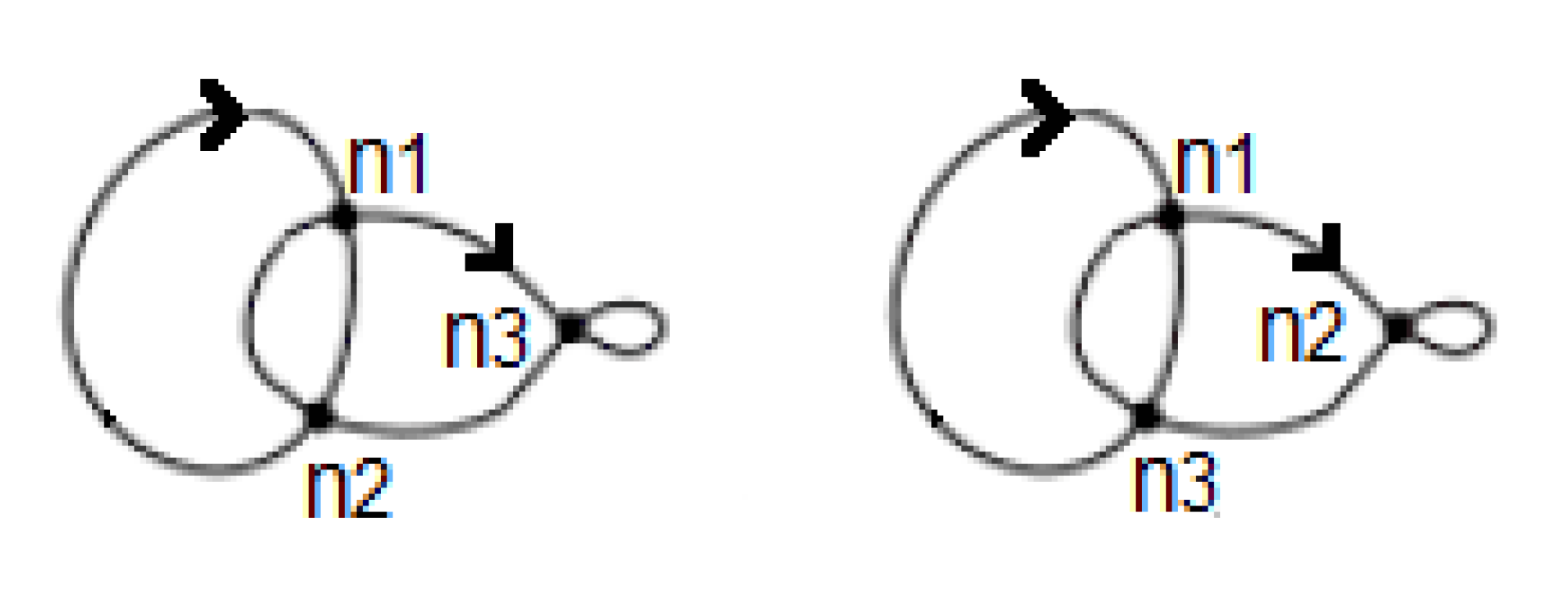
We also define the sticking chord diagram in a similar way chord diagrams are defined for oriented singular knots, but with oriented chords in a way similar to that of Gauss diagrams of usual knots. See Figure 3 for an example of two stuck knots with the same sticking chord diagram.

The aim of this research is to develop the beginnings of a theory of what we calls stuck knots, which one can think of as closed loops of rope in space which are allowed to be glued to themselves at various points. Then we show that this has its connections and applications in the topology of RNA folding as an example. Connections with other biological objects are very likely. Connections with other physical objects are possible.

This paper is organized as follows. In Section 2, we introduce some preliminaries focusing on Jones polynomial invariant and its definition using Kauffman bracket. In Section 3, we introduce an invariant of stuck knots and links, and we study the symmetry of stuck knots based on mirror imaging. In Section 4, we give an invariant of singular knots by inserting stuck crossing at the singularities of a singular knot. In Section 5, we introduce the concepts of stuckness factor and relatively stuck knots and we give an invariant of such knots. In Section 6, we give applications of stuck knots and links and their invariants in modeling and understanding bonded RNA foldings, and we explore the topology of such objects with invariants involving multiplicities at the bonds. In Section 7, some perspectives and ideas are discussed.

2. Preliminaries

In 1984, Vaughan Jones gave his revolutionary new polynomial invariant for knots and links in [7]. This polynomial opened a wide area of applications to many branches of mathematics and physics. The Jones polynomial succeeded to distinguish many different knots and links that could not be distinguished by other invariants including the well-known Alexander invariant.

Louis Kauffman defined the Jones polynomial in a very natural way using his revolutionary bracket polynomial [2]. In this section, we give the Jones polynomial as defined by Louis Kauffman in terms of his bracket polynomial. Then a simple change of the variable will give the original Jones polynomial. We will be following mainly the methodology of [2] in defining the Jones polynomial.

Definition 1.

For an oriented diagram D of a link L, the Kauffman bracket is a polynomial in $\mathbb{Z}\left[A,A^{-1}\right]$ for the unoriented diagram $\left|D\right|$, denoted by $〈\left|D\right|〉$, and characterized by the rules:

1.

= A + A⁻¹

2.

= (−A²−A⁻²)〈|D|〉

3.

= 1

A crossing in an oriented diagram D has a sign of $+1$ or $-1$ according to the right-hand rule. The sum of signs of the crossings for a given diagram D is called the writhe of D and is denoted by $w\left(D\right).$

Theorem 1.

Let D be a an oriented link diagram. Then the X polynomial defined by

$$X\left(D\right)={(-A)}^{-3w\left(D\right)}〈\left|D\right|〉$$

(1)

is an invariant of links.

Definition 2.

The Jones polynomial $V\left(L\right)$ of an oriented link L with diagram D is the Laurent polynomial in the indeterminate $q.$ With integer coefficients, defined by

$$V\left(L\right)={\left({(-A)}^{-3w\left(D\right)}〈\left|D\right|〉\right)}_{q^{-1/4}=A}\in \mathbb{Z}[q^{-1},q]$$

(2)

Sometimes $X\left(D\right)$ is also referred to as the Jones polynomial in terms of A, as it is equivalent to $V\left(L\right).$

3. A Polynomial Invariant of Stuck Knots

Definition 3.

For an oriented diagram D of a stuck link L, the bracket is a polynomial in $\mathbb{Z}\left[A,A^{-1},x,y\right]$ denoted by $〈\left|D\right|〉$ and characterized by the rules:

1.

= x + y

2.

= A + A⁻¹

3.

= (−A² − A⁻²) 〈|D|〉

4.

= 1

Theorem 2.

The bracket of stuck knots is invariant under the R2, R3, S2, and S3 moves

Proof. 

We know that Kauffman bracket is invariant under the regular Reidemeister moves R2 and R3. So all we have to do is to prove that this bracket is invariant under the stuck moves as follows.

For the S2 moves we have

For the S3 moves we have

We have considered two of four cases of each of the $S2$ and $S3$ moves, as the other two cases can be proved similarly for each of them. This completes the proof. □

The following theorem follows immediately.

Theorem 3.

Let D be a an oriented stuck link diagram. Then the $\widehat{X}$ polynomial defined by

$$\widehat{X}\left(D\right)={(-A^3)}^{-w\left(D\right)}〈\left|D\right|〉$$

(3)

is an isotopy invariant of oriented stuck links, where $w\left(D\right)$ is the usual writhe, that is the sum of signs of the usual crossings.

It is well-known that the X polynomial of usual links satisfies the following skein relation

A⁴X − A⁻⁴X = (A⁻²− A²) X ,

(4)

which is still satisfied by our generalized $\widehat{X}$ polynomial. However, another skein relation involving stuck crossings is given in the following lemma.

Lemma 1.

$x\widehat{X}$ $-y\widehat{X}$ $=\left(x^2-y^2\right)\widehat{X}$ .

Proof. 

Multiplying the following equation by x

= x + y ,

and the following equation by y

= y + x ,

and subtracting the results, we get

x − y = (x² − y²) ,

and since the writhe does not involve the signs of stuck crossings, the links , , and will have equal writhe say $\omega$. Therefore, by multiplying the last equation by ${(-A^3)}^{-\omega }$, we get

x − y = (x² − y²) .

□

Definition 4.

A stuck link is said to be completely stuck if it has a diagram with only stuck crossings.

As the writhe of a completely stuck link is zero, we have $\widehat{X}\left(D\right)=〈\left|D\right|〉$ and the following corollary follows.

Corollary 1.

The bracket is an isotopy invariant of completely stuck links.

The Jones polynomial of usual oriented links can not distinguish an oriented knot from the same knot with the reversed orientation, but, sometimes, it can distinguish between an oriented link (of more than one component) and the same link with reversed orientation on one of its components. The $\widehat{X}$ polynomial above does not change with any change of orientation in completely stuck links, because $\widehat{X}\left(D\right)=〈\left|D\right|〉.$

Definition 5.

The mirror image of a stuck link K is the stuck link $K^{*}$ with diagram $D^{*}$ obtained from a diagram D of K by changing every usual crossing to the opposite crossing and every stuck crossing to the opposite crossing (That is shifting the label A to an adjacent region). A stuck link that is isotopic to its mirror image will be called amphechiral.

It is well-known that if K is a usual link, then $X\left(K^{*}\right)$ can be obtained from $X\left(K\right)$ by replacing every A by $A^{-1}.$

Lemma 2.

For a stuck link K, $\widehat{X}\left(K^{*}\right)$ can be obtained from $\widehat{X}\left(K\right)$ by replacing every A by $A^{-1}$ and every x by y and every y by x.

Proof. 

This can be easily seen by the definition of the $\widehat{X}$ polynomial and the bracket. □

Example 1.

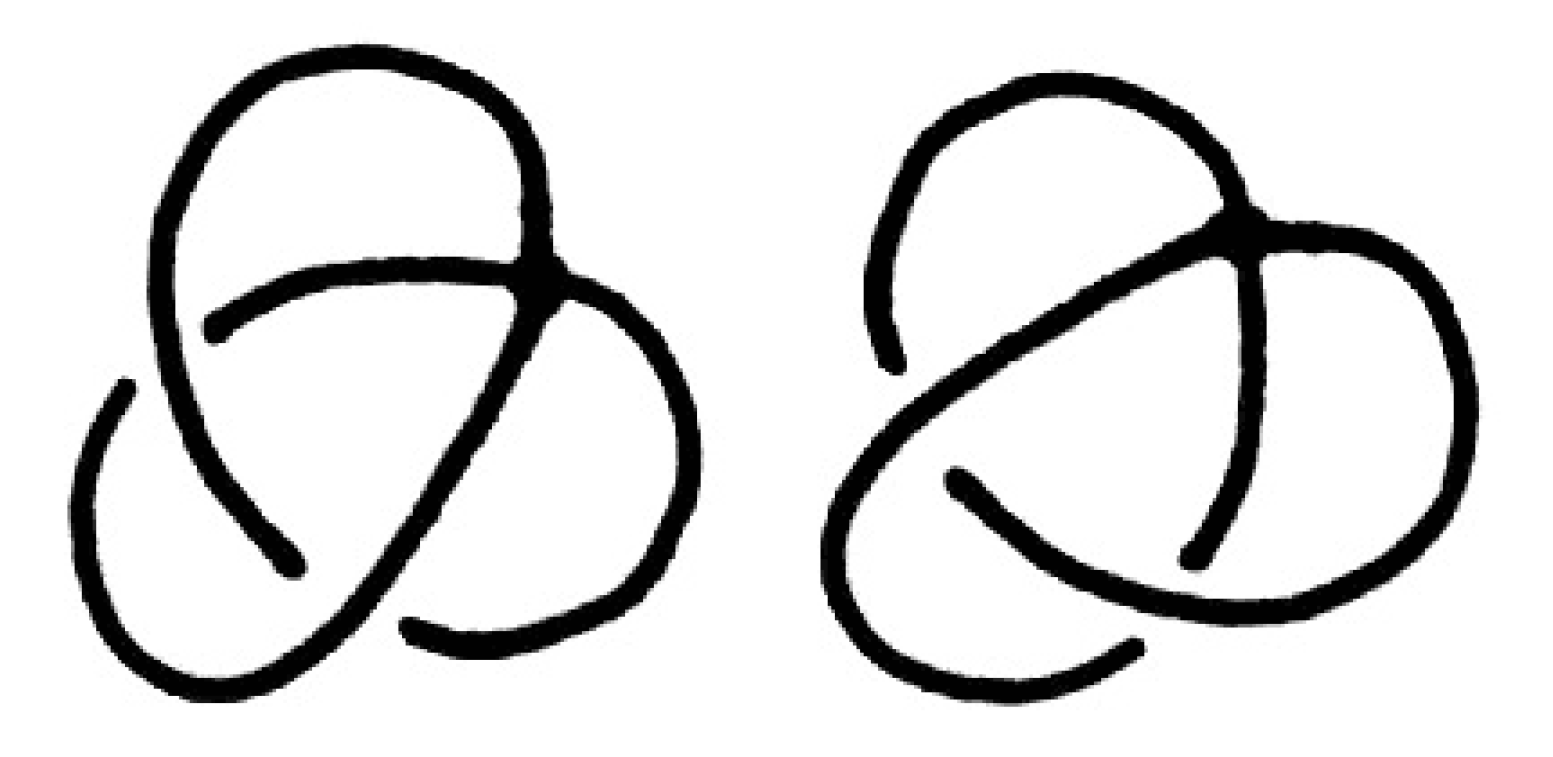
The following two completely stuck knots are not isotopic as we see by their polynomials.

therefore they are not isotopic, and hence not amphechiral, as they are mirror images for each other. We will refer to these two stuck knots by the right stuck infinity and the left stuck infinity, respectively. Note that these two stuck knots can also be distinguished by their signed sticking numbers given by$+1$and$-1$, respectively.

Example 2.

The following two stuck knots are not isotopic as we see by their polynomials

in spite of the fact that they have equal signed sticking numbers.

Example 3.

The following two completely stuck links can not be distinguished by the $\widehat{X}$ polynomial, but they have different linking sticking numbers of $-2$ and 2, respectively.

Example 4.

The following two completely stuck links are, in fact, isotopic, which can be seen by a vertical flip followed by a horizontal flip of one of the two stuck links.

It is also well-known that the Kauffman bracket polynomial of a usual link with diagram D satisfies the following so-called state sum formula

$$〈\left|D\right|〉=\sum _S{A}^{a\left(S\right)-b\left(S\right)}{\left(-A^2-A^{-2}\right)}^{\left|S\right|-1},$$

(5)

where S is a what results from smoothing all the crossings of the diagram $\left|D\right|$ by making only one smoothing choice at each crossing (either A- split or B-split).

$\left|S\right|$ is the total number of circles in S, $a\left(s\right)$ is the total number of A-splits in state S, $b\left(s\right)$ is the total number of B-splits in state S.

A similar state sum formula can be obtained for the generalized bracket of stuck knots. It is easy to see that if D is a stuck link diagram, then the generalized bracket is given by

$$〈\left|D\right|〉=\sum _S{A}^{a\left(S\right)-b\left(S\right)}{x}^{\alpha \left(S\right)}{y}^{\beta \left(S\right)}{\left(-A^2-A^{-2}\right)}^{\left|S\right|-1},$$

(6)

where $\alpha \left(S\right)$ is the number of A-splits of stuck crossings in state S, and $\beta \left(S\right)$ is the number of B-splits of stuck crossings in a state $S.$

Note that if a stuck link is completely stuck with diagram D involving only stuck crossings, then

$$〈\left|D\right|〉=\sum _S{x}^{\alpha \left(S\right)}{y}^{\beta \left(S\right)}{\left(-A^2-A^{-2}\right)}^{\left|S\right|-1}=\widehat{X}\left(D\right).$$

(7)

Note that $\alpha \left(S\right)+\beta \left(S\right)$ is equal to the number of stuck crossings, say $\alpha \left(S\right)+\beta \left(S\right)=n$. Let $\delta =-A^2-A^{-2}$, then we get

$$\widehat{X}\left(D\right)=\sum _S{x}^{\alpha \left(S\right)}{y}^{\beta \left(S\right)}{\delta }^{\left|S\right|-1}.$$

(8)

Note that $\widehat{X}\left(D\right)$ can be rewritten as follows

$$\widehat{X}\left(D\right)=\underset{i=0}{\sum ^n}{P}_i\left(\delta \right)x^i{y}^{n-i},$$

(9)

where each $P_i$ is a polynomial (with non-negative powers) of $\delta$. Note that $\delta$ is a palindromic Laurent polynomial in A (that is to say if each A is replaced by $A^{-1}$, we get the same result). It is an easy exercise to show that each $P_i\left(\delta \right)$ is also a palindromic Laurent polynomial in terms of A. Now we have evidence for the following theorem.

Theorem 4.

If L is a completely stuck link, and

$$\widehat{X}\left(L\right)=\underset{i=0}{\sum ^n}{P}_i\left(\delta \right)x^i{y}^{n-i},$$

(10)

as described above, then each $P_i\left(\delta \right)$ is a palindromic Laurent polynomial in terms of A.

Example 5.

The following stuck link is not completely stuck, as $A^6$ is not palindromic.

4. A Stuck Crossing Insertion Invariant for Singular Knots

Singular links can be thought of as stuck links with no information of which strand is over the other at the stuck crossings. Singular links are subject to the same Reidemeister-like moves of stuck knots given in the introduction of this article, but without the letters marking the A-regions. Note that by deleting the A-marks in a stuck link diagram we get a singular link diagram. The following lemma is obvious now.

Lemma 3.

If two stuck links are isotopic, then they are isotopic as singular links.

If a singular link diagram has n vertices, then there are $2^n$ ways to get stuck links of it, as there are two possibilities for the A-mark at each vertex. Each way of the $2^n$ ways will be called an A-marking of the singular link. We give the following lemma.

Lemma 4.

If $K_1$ and $K_2$ are isotopic singular link diagrams, then for each A-marking of $K_1$ inducing a stuck link diagram $K_1^{*}$ there exist an A-marking of $K_2$ inducing $K_2^{*}$ such that $K_2^{*}$ is isotopic to $K_1^{*}$.

Proof. 

It is obvious that a similar sequence of Reidemeister-like moves turning $K_1$ into $K_2$ will turn the A-marked diagram $K_1^{*}$ into an A-marked diagram say $K_2^{*}$. This diagram $K_2^{*}$ has the required A-marking. □

Therefore, by this theorem, if we have two singular link diagrams $D_1$ and $D_2$ with equal number of vertices and if there is an A-marking of $D_1$ that is not isotopic to any marking of $D_2$, then $D_1$ and $D_2$ are not isotopic as singular links.

Example 6.

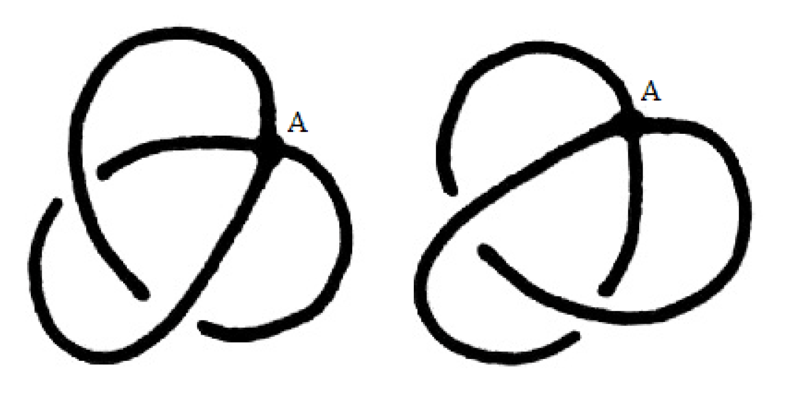
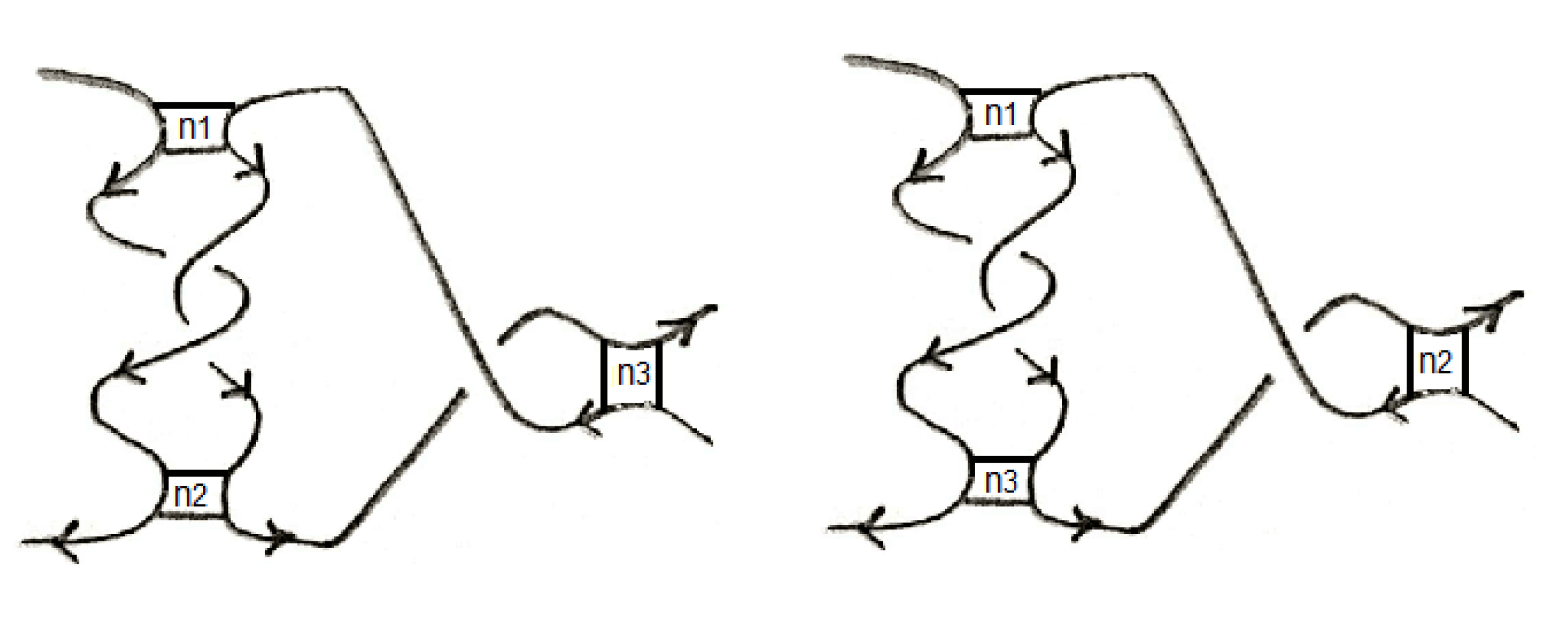
The following two singular knots are not isotopic. See Figure 4.

As we can see by the following calculations and the last lemma

Remark 1.

In fact we can reduce the possibilities of markings of $K_2$, which make $K_2^{*}$ isotopic to $K_1^{*}$. This can be done by excluding all markings of $K_2$ yielding different signed sticking number and linking sticking number from that of $K_1^{*}$. Therefore, in the last example, all we need to compute is the polynomial $\widehat{X}$ for the stuck knots in Figure 5 in order to tell the corresponding singular knots apart.

Among all possible A-markings of a singular link diagram we describe the following for an oriented singular link. Replace each vertex by a positive stuck crossing; that is to say put the A-markings in the regions lying between strands with both arrows heading into or out of the vertex. We will refer to this marking by the positive marking. Another marking that can be given canonically is the negative marking, which is the result of replacing each vertex by a negative stuck crossing. One can think of other markings considering the configurations and the chord diagrams in some classes of singular knots.

As a result we can define an invariant of singular links based on the positive marking and using our $\widehat{X}$ polynomial of stuck links.

Theorem 5.

For a diagram D of an oriented singular link L, let the positive-marking bracket denoted by $〈D〉$ be characterized by the rules:

1.

= x + y

2.

= A + A⁻¹

3.

= (−A² − A⁻²) 〈|D|〉

4.

= 1

Then the ${\widehat{X}}_{+}$ polynomial defined by

$${\widehat{X}}_{+}\left(D\right)={(-A^3)}^{-w\left(D\right)}〈\left|D\right|〉$$

(11)

is an isotopy invariant of oriented singular links, where $w\left(D\right)$ is the usual writhe, that is the sum of signs of the usual crossings.

In fact this invariant coincides with an invariant defined by H. Dye in [8].

5. Stuckness Factors and Relatively Stuck Knots

Let K be a physical stuck knot (or link) that is made out of wire or rope of any material. Let s be a stuck crossing in the stuck knot diagram. Let $t\in \left[0,1\right]$ be a number (that refers to the stuckness of the crossing) on a scale of real numbers in the interval $\left[0,1\right]$. When $0<t<1$ we replace the letter A indicating the A-regions by this t for two purposes; the first is to indicate the A-regions and the second is to refer to the stuckness of the crossing. When $t=0,$ the crossing is a usual crossing and we have the option to mark the crossing by the number 0 in the A-regions with replacing the crossing by a double point, or leave the usual crossing as it appears in usual knot diagrams. When $t=1$, the crossing is a singular crossing and we might put 1 in any region around the double point, as at a singular crossing no strand is over the other. We have the option not to mark this singular crossing by the number 1 leaving it implicitly understood by the unmarked vertex. We call the number t the stuckness factor of the crossing $s.$

Let D be a stuck knot diagram with stuck crossings $s_1,\dots ,s_n$ labeled by the stuck factors $t_1,\dots ,t_n$, respectively. We will call such knots relatively stuck knots. We define the isotopy of relatively stuck knots using the same Reidemeister-like moves of usual stuck knots, but we require that the stuckness factor at each stuck crossing be preserved; that is, the $S2$ and $S3$ moves should preserve the stuck factor assigned to each stuck crossing.

The following theorem provides us with an invariant of relatively stuck knots.

Theorem 6.

Let D be a diagram of an oriented relatively stuck knot or link L, and the bracket of $\left|D\right|$ denoted by $〈\left|D\right|〉$ be characterized by the rules:

1.

= A^1−t + A^t−1

2.

= (−A²−A⁻²)〈|D|〉

3.

= 1

then $Y\left(D\right)$ defined by

$$Y\left(D\right)={(-A^3)}^{-w\left(D\right)}〈\left|D\right|〉$$

(12)

is an isotopy invariant, where $w\left(D\right)$ is the usual writhe, that is the sum of signs of the usual crossings (or equivalently the stuck crossings with zero stuckness factor).

Proof. 

At usual crossings $(t=0),$Y acts like the usual Jones polynomial defined via Kauffman bracket. At singular knots $(t=1)$ it is a simple generalization of Jones polynomial to singular knots. At stuck crossings with $0<t<1,$Y is just the $\widehat{X}$ polynomial, defined in the previous section for stuck knots, with $x=A^{1-t}$ and $y=A^{t-1}$. Therefore Y is an invariant of relatively stuck knots. □

Example 7.

The following two relatively stuck links (denoted by K and $L,$ respectively) are identical except for the order of the stuckness factors given unspecifically by $t_1,$$t_2,$ and $t_3$. Note that if $t_2=t_3$, then the two links are isotopic. See Figure 6.

Calculations of the Y invariant give the following results

$$\begin{array}{ccc}\hfill Y\left(K\right)& =& A^{7-\left(t_1+t_2+t_3\right)}+A^{-1-\left(t_1+t_2+t_3\right)}+2A^{3-\left(t_1+t_2+t_3\right)}-A^{3-t_1-t_2+t_3}\hfill \\ & & -A^{3-t_1+t_2-t_3}-A^{3+t_1-t_2-t_3}-A^{-1+\left(t_1+t_2+t_3\right)}-A^{-1-t_1-t_2+t_3}\hfill \\ & & -A^{-1-t_1+t_2-t_3}-A^{-1+t_1-t_2-t_3}-A^{-5+\left(t_1+t_2+t_3\right)}+A^{-1-t_1+t_2+t_3}\hfill \\ & & +A^{3+t_1+t_2-t_3}+A^{-5+t_1+t_2-t_3}+2A^{-1+t_1+t_2-t_3}+A^{-1+t_1-t_2+t_3}\hfill \end{array}$$

and

$$\begin{array}{ccc}\hfill Y\left(L\right)& =& A^{7-\left(t_1+t_2+t_3\right)}+A^{-1-\left(t_1+t_2+t_3\right)}+2A^{3-\left(t_1+t_2+t_3\right)}-A^{3-t_1-t_2+t_3}\hfill \\ & & -A^{3-t_1+t_2-t_3}-A^{3+t_1-t_2-t_3}-A^{-1+\left(t_1+t_2+t_3\right)}-A^{-1-t_1-t_2+t_3}\hfill \\ & & -A^{-1-t_1+t_2-t_3}-A^{-1+t_1-t_2-t_3}-A^{-5+\left(t_1+t_2+t_3\right)}+A^{-1-t_1+t_2+t_3}\hfill \\ & & +A^{3+t_1-t_2+t_3}+A^{-5+t_1-t_2+t_3}+2A^{-1+t_1-t_2+t_3}+A^{-1+t_1+t_2-t_3}\hfill \end{array}$$

Note that we have rearranged the terms so that the first twelve terms in $Y\left(K\right)$ are the same as the first twelve terms in $Y\left(L\right).$ The last four terms in each of them will be equal if and only if $t_2=t_3$. Therefore if $t_2\ne t_3$, then the two links are not isotopic. Hence these two links are not isotopic if and only if $t_2\ne t_3$.

6. Applications

In [9] Kauffman and Magarshak introduced combinatorial structures into the study of RNA folding. These structures are useful for the classification of the embeddings of these foldings into three dimensional space.

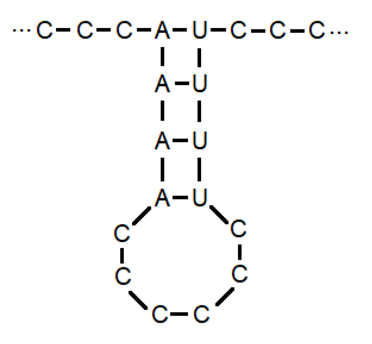
An RNA molecule is a long chain consisting in a sequence of the bases A (adenine), C (cytosine), U (uracil) and G (guanine). The pairs (A and U) and (C and G) are capable of bonding with each other. A folding of an RNA molecule is a possible pairing structure with respect to the given sequence of bases of the RNA molecule. For example the folding corresponding to the chain $\cdots CCCAAAACCCCCUUUUCCC\cdots$ is given as shown in Figure 7.

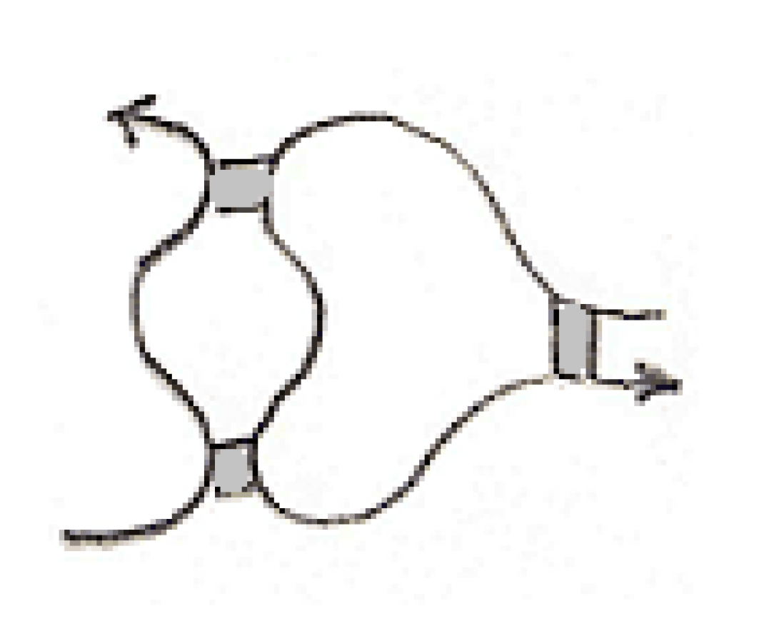
This folding may be abstracted to a diagram that indicates the form of the pairing as shown below in Figure 8.

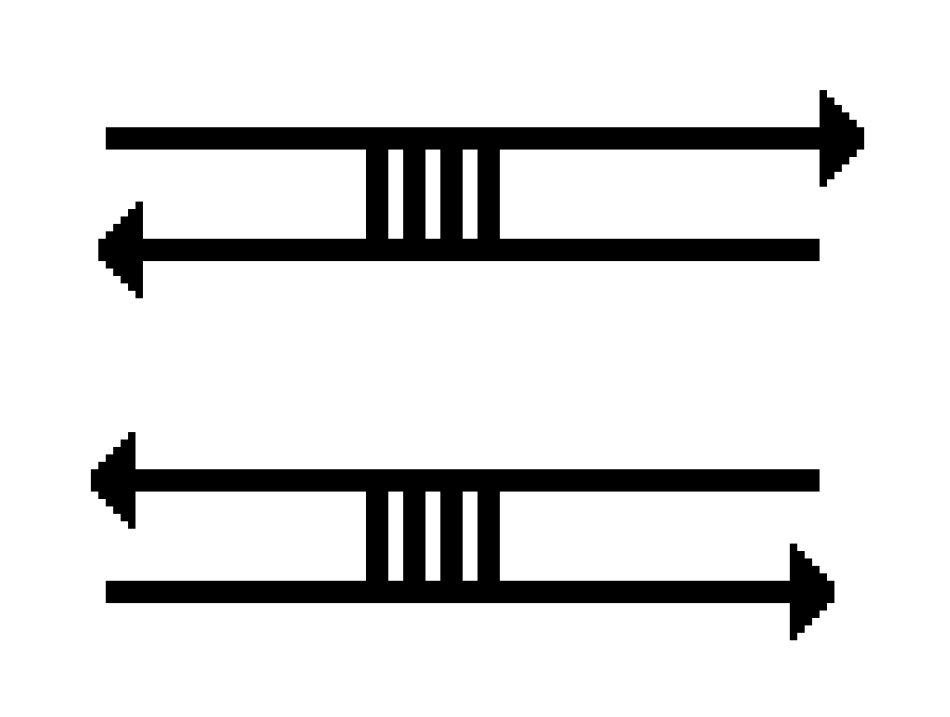
In the diagram above we obtained one basic pairing node represented by the connecting arcs. A basic pairing node is one of the two in Figure 9.

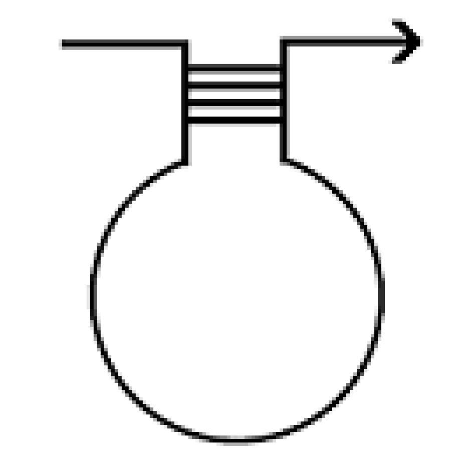
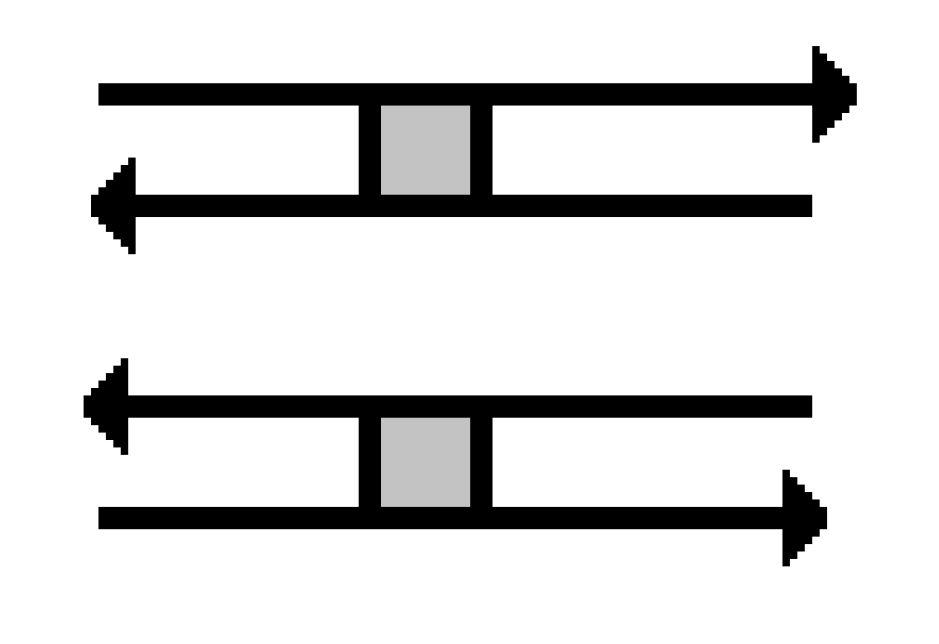
Where the directions of the arcs are always opposite, Any multiplicity of connecting arcs is possible but Kauffman and Magarshak adopted the connection of four such arcs for pictorial purposes. We will adopt a gray strip in place of the four connecting arcs so that a pairing node looks as one of the following, see Figure 10.

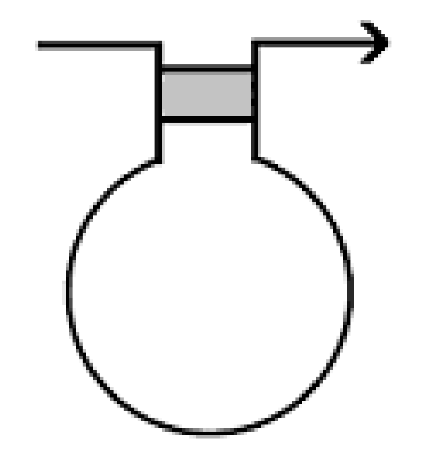
Furthermore, the folding diagram of the chain $\cdots CCCAAAACCCCCUUUUCCC\cdots$ looks as shown below in Figure 11.

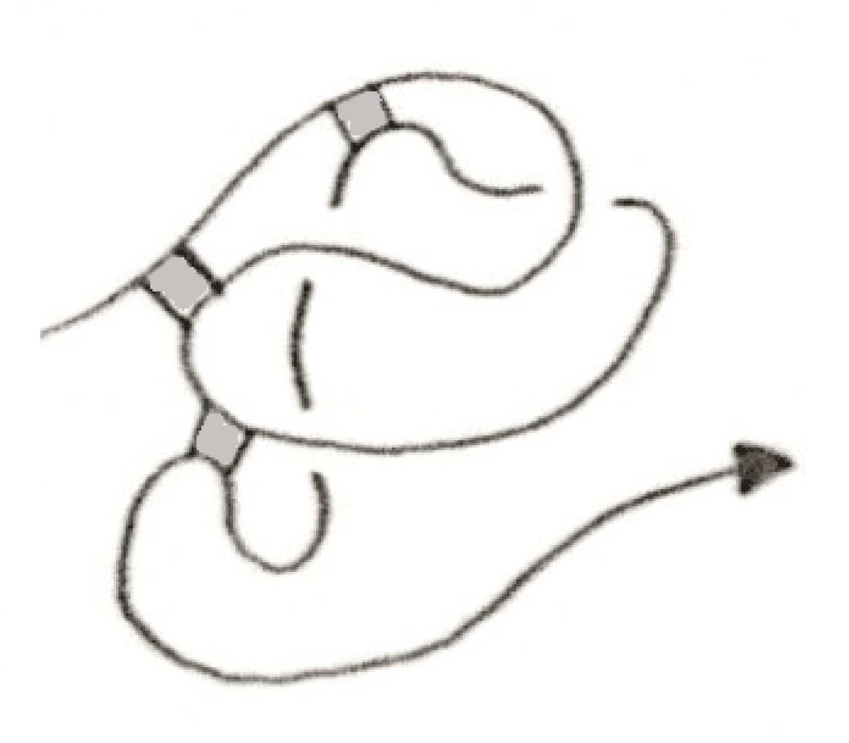
An example of an arc diagram of RNA folding in three dimensional space is given below in Figure 12.

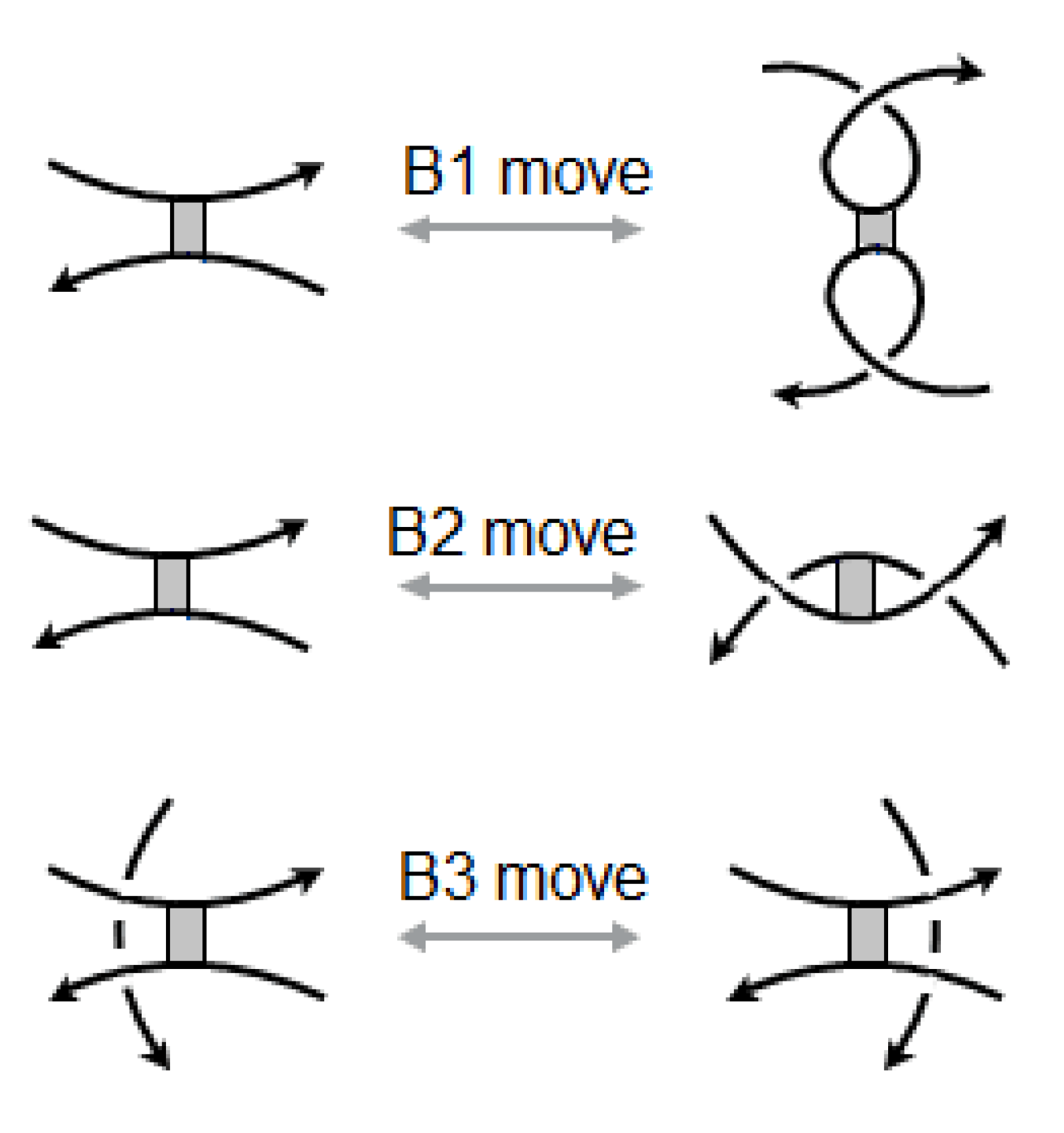
Kauffman and Magarshak introduced an appropriate mathematical model for the topology of RNA. A pairing node has been called a bond vertex. A bond vertex is taken to be a rigid vertex in the sense that the configuration of the bonding arcs is rigid (not subject to any twisting), while the oriented arcs are topologically flexible. Therefore arc diagrams of RNA folding are subject to the usual Reidemeister moves and the following moves in Figure 13, besides obvious symmetries obtained by their mirror imaging. See [9].

6.1. Transforming an Arc Diagram of RNA Folding to a Stuck Arc Diagram

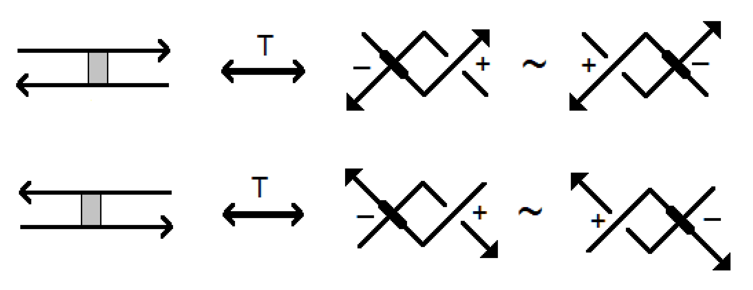
Now we introduce a way to transform between an arc diagram of RNA folding and what we call a stuck arc diagram with negative stuck crossings as shown below in Figure 14.

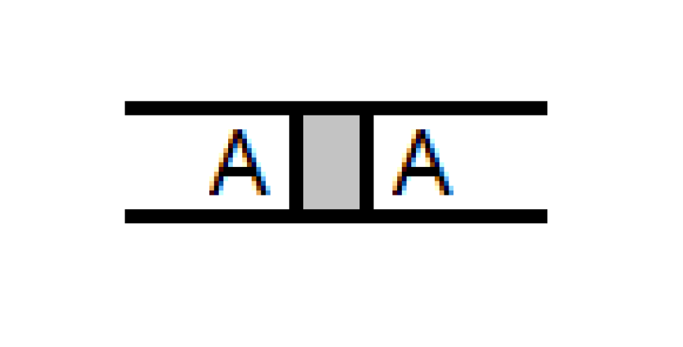
The idea of this transformation T is to hide the strip of the bond vertex by rotating it around the bonded strands. This flexibility of rotation is deduced formally from move B2 introduced before and given by Kauffman and Magarshak, as one can see that move B2 can not be performed without this flexibility of rotation of the strip of the bond vertex. One way to see this transformation abstractly is by deleting the strip in a bond vertex then overlapping the two strands via a Reidemeister move II, then converting the negative crossing to a negative stuck crossing, while keeping the positive crossing unstuck. Another way to see this transformation is by using the A-regions notation. First of all we denote the two inner regions on the two sides of a bond vertex by the A-regions as in Figure 15.

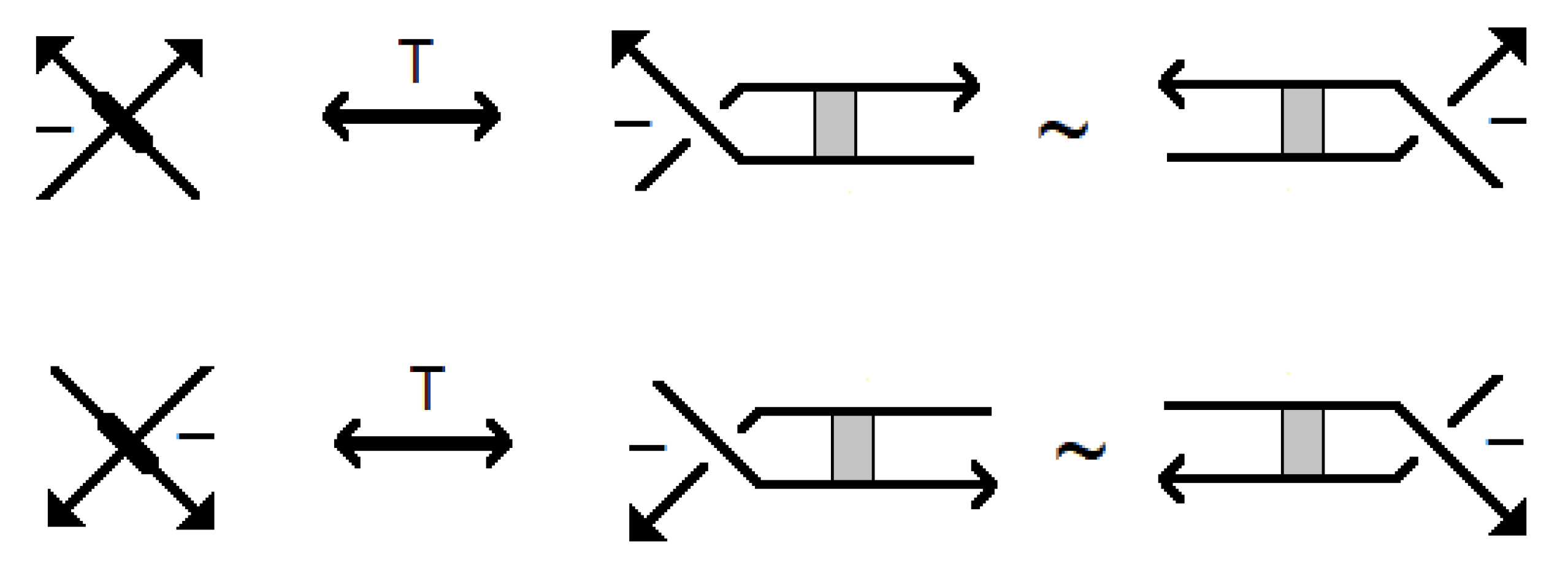
After deleting the rectangular strip we overlap the two strands via a Reidemeister move II, and convert the crossing that preserves the horizontality of the A-regions into a stuck crossing, while we keep the other crossing with vertical A-regions unchanged. Figure 16 shows the same transformation starting with negative stuck crossings

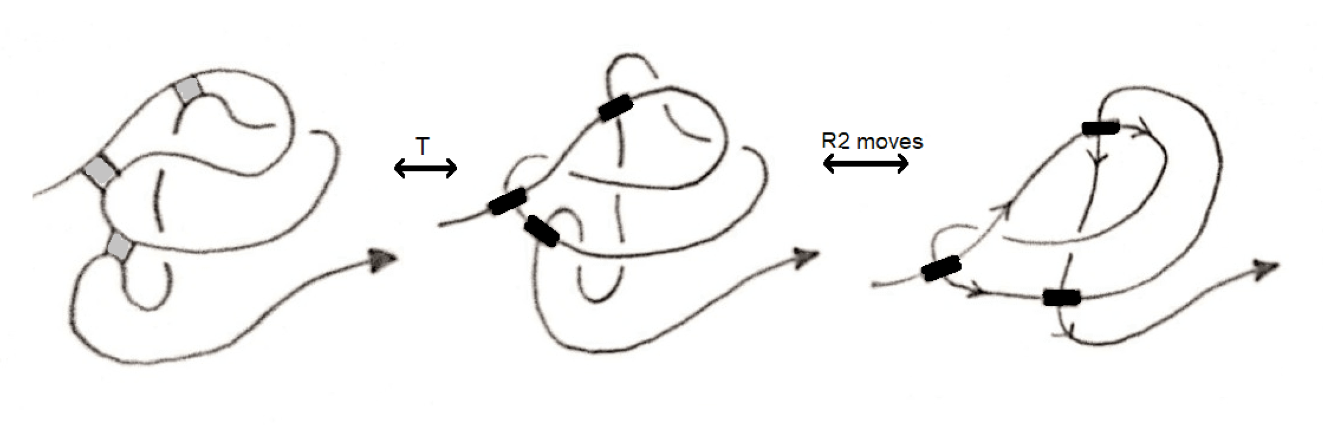
See Figure 17 for transforming between an RNA folding arc and what we called a stuck arc diagram.

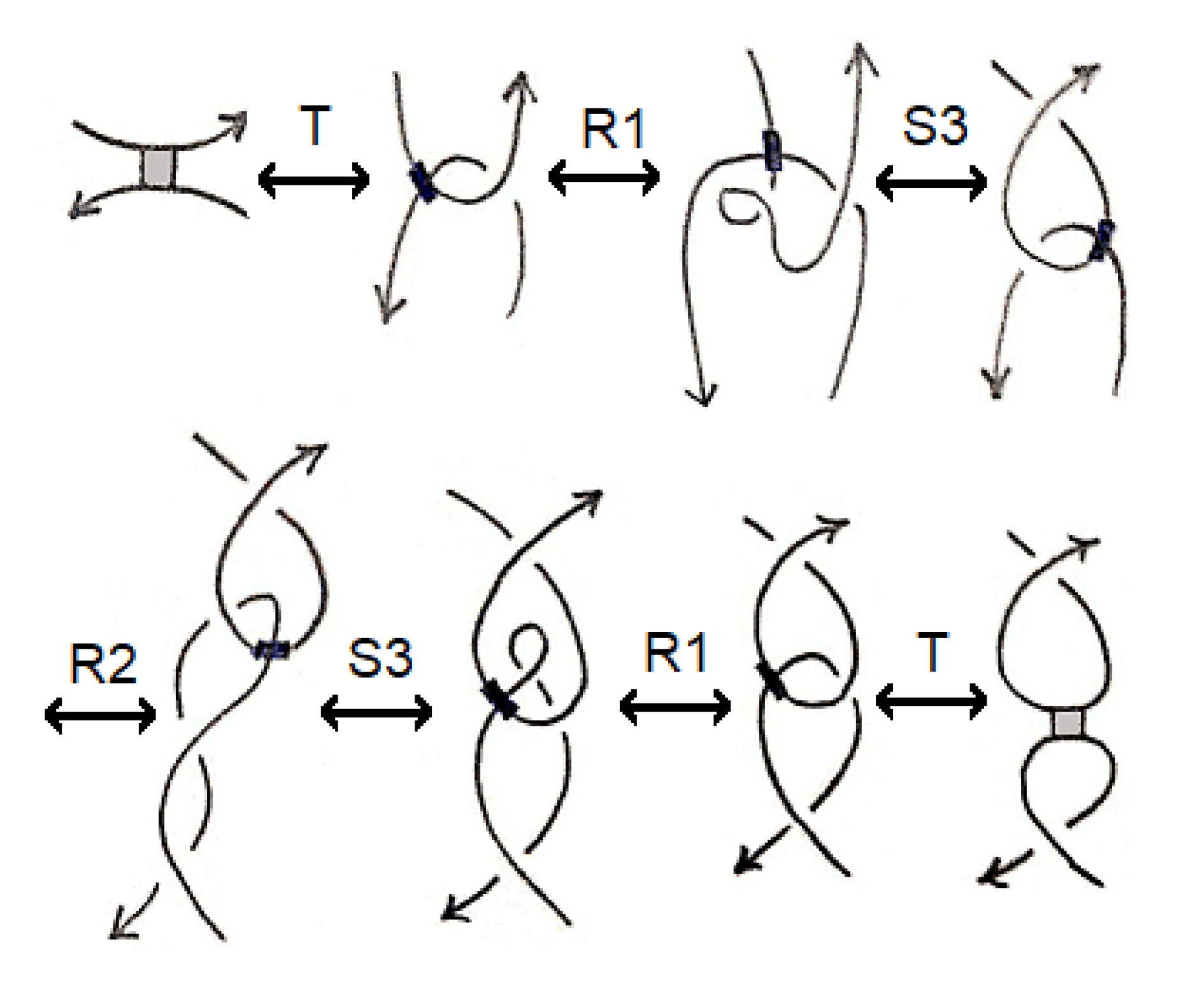
It is easy to see that in the presence of the usual three Reidemeister moves we can get the bond vertex moves B1, B2 and B3 from the three stuck crossing moves S1, S2 and S3 and vice versa under the transformation T. Figure 18 shows how to deduce the move B1 using the stuck crossing moves and the Reidemeister moves.

This should not be hard to expect as both the stuck crossing moves and the Reidemeister moves are ones that simulate the rigid vertex moves of singular knots.

In [10] a model of knot polynomials to characterize RNA structures has been developed by Tian, Lei, Kauffman, and Liang. At first, they closed off RNA strands into circles. For RNA structures with a single strand, the backbone trace, represented by the arc of the RNA folding arc, is closed off by connecting the ends virtually. RNA structures might involve multiple strands, and bond vertices of two types. Other than the bond vertices in each single strand there can be bond vertices connecting several strands as in Figure 19 for an RNA folding diagram with two arcs.

Such structures are also considered subject to the three bond vertex diagrams B1, B2 and B3. In this case the strands can be closed in several ways. However, in [10], they closed RNA strands using the self–closure approach; that is the two ends of each arc are connected virtually. Then they defined a polynomial invariant called the Simplified RNA Polynomial (SiRP) via what they call the simplified skein relation, which inserts two specific usual tangles in place of each bond vertex so that they get a specific combination of usual knots and links and consequently a polynomial in three variables.

Now we will utilize our $\widehat{X}$ polynomial to serve the topology of RNA structure. At first we use the transformation T to transform a given RNA structure arc diagram into a stuck arc diagram, then we close the diagram using the self closure. Then we can apply our $\widehat{X}$ polynomial defined in Section 3 on the resulting oriented stuck knot or link. Therefore $\widehat{X}$ acts as a model of knot polynomials to characterize RNA structures.

Example 8.

To compute $\widehat{X}$ for the RNA arc diagram we compute $\widehat{X}$ for the stuck knot and hence we get

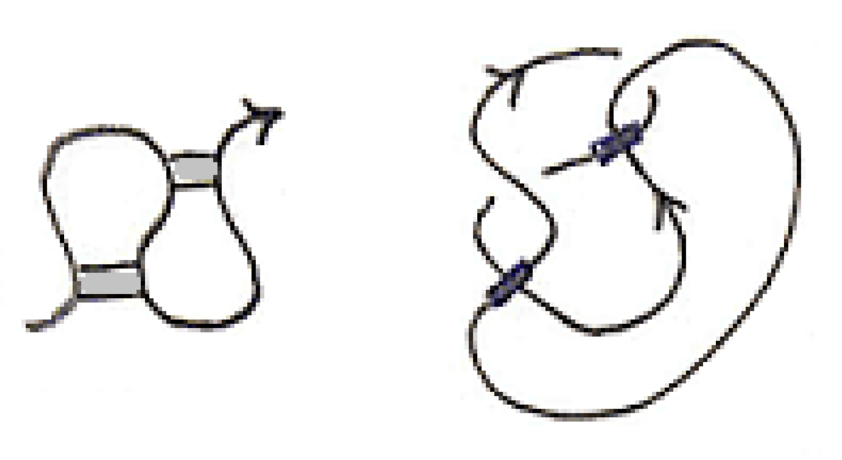
Example 9.

Figure 20 involves an RNA folding arc diagram and the corresponding closed stuck diagram

The $\widehat{X}$ polynomial of this RNA folding arc is $x^2+xy+xy{A}^{-6}+y^2$

6.2. A Polynomial for an RNA Folding Involving Vertex Multiplicities

We now give an invariant of an RNA folding with given multiplicities. As we know a gray rectangle represents a bond vertex. This gray rectangle might contain any natural number representing the multiplicity of connecting arcs. As we saw in Section 5, we could involve real numbers (in that section real numbers between 0 and 1) in what we called relatively stuck knots, and we could define an invariant of such knots that involved these numbers. Now we will consider RNA arc diagrams with given natural numbers in their gray rectangles. We will transform them into stuck arc diagrams with the natural numbers put in the A-regions at each stuck crossing. Then we close them to stuck knots and links via the self closure process described before. Then we have a new invariant that takes these multiplicities into consideration as in the following theorem.

Theorem 7.

Let D be a diagram of an oriented stuck knot or link L with stuck crossings involving multiplicities in $\mathbb{N}$, and the bracket of $\left|D\right|$ denoted by $〈\left|D\right|〉$ be characterized by the rules:

1.

= A + A⁻¹

2.

= A¹⁻ⁿ + Aⁿ⁻¹

3.

= (−A² − A⁻²) 〈|D|〉

4.

= 1

then $\widehat{Y}\left(D\right)$ defined by

$$\widehat{Y}\left(D\right)={(-A^3)}^{-w\left(D\right)}〈\left|D\right|〉$$

(13)

is an isotopy invariant, where $w\left(D\right)$ is the usual writhe, that is the sum of signs of the usual crossings.

Proof. 

The proof of this theorem follows directly from the proof of Theorem 6 in Section 5 as there is nothing special about the numbers at the stuck crossings being natural or real numbers between 0 and 1. □

Example 10.

The following two stuck links with multiplicities (denoted by K and $L,$ respectively) are identical except for the order of the multiplicities given unspecifically by $n_1,$$n_2,$ and $n_3$. Note that if $n_2=n_3$, then the two links are isotopic. See Figure 21.

These two stuck links correspond to the following two RNA folding diagrams, respectively (see Figure 22).

Calculations of the $\widehat{Y}$ invariant give the following results

$$\begin{array}{ccc}\hfill Y\left(K\right)& =& A^{-7-\left(n_1+n_2+n_3\right)}+A^{1+\left(n_1+n_2+n_3\right)}+2A^{-3+\left(n_1+n_2+n_3\right)}-A^{1-n_1+n_2+n_3}\hfill \\ & & -A^{-3-n_1+n_2+n_3}-A^{1+n_1-n_2-n_3}-A^{5-(n_1+n_2+n_3)}-A^{1-(n_1+n_2+n_3)}\hfill \\ & & -A^{-3+n_1+n_2-n_3}-A^{-3+n_1-n_2+n_3}-A^{1+n_1+n_2-n_3}-A^{1+n_1-n_2+n_3}\hfill \\ & & +A^{-3-n_1-n_2+n_3}+A^{5-n_1-n_2+n_3}+2A^{1-n_1-n_2+n_3}-A^{1-n_1+n_2-n_3}\hfill \end{array}$$

and

$$\begin{array}{ccc}\hfill Y\left(L\right)& =& A^{-7-\left(n_1+n_2+n_3\right)}+A^{1+\left(n_1+n_2+n_3\right)}+2A^{-3+\left(n_1+n_2+n_3\right)}-A^{1-n_1+n_2+n_3}\hfill \\ & & -A^{-3-n_1+n_2+n_3}-A^{1+n_1-n_2-n_3}-A^{5-(n_1+n_2+n_3)}-A^{1-(n_1+n_2+n_3)}\hfill \\ & & -A^{-3+n_1+n_2-n_3}-A^{-3+n_1-n_2+n_3}-A^{1+n_1+n_2-n_3}-A^{1+n_1-n_2+n_3}\hfill \\ & & +A^{-3-n_1+n_2-n_3}+A^{5-n_1+n_2-n_3}+2A^{1-n_1+n_2-n_3}-A^{1-n_1-n_2+n_3}\hfill \end{array}$$

We have rearranged the terms so that the first twelve terms in $Y\left(K\right)$ are the same as the first twelve terms in $Y\left(L\right).$ The last four terms in each of them will be equal if and only if $n_2=n_3$. Therefore if $n_2\ne n_3$, then the two links are not isotopic. Hence these two links are not isotopic if and only if $n_2\ne n_3$.

7. Discussion

Given this framework of thinking in stuck knots and developing their invariants, there are other perspectives to be thought of. We provide the reader with the following ideas:

(1)

In modeling RNA folding diagrams we have considered a transformation T that inserts a negative stuck crossing and a positive usual crossing in place of a bond vertex with antiparallel strands. If a bond vertex with parallel strands is to be considered in other similar biological objects (such as DNA and proteins), then one can insert a positive stuck crossing and a negative usual crossing in place of each bond vertex with parallel strands.

(2)

There was nothing special with negative stuck crossings replacing bond vertices with antiparallel strands.

(3)

A geometer might be interested in singular knots with singular points having non-right but equal opposite angles. In this case the A-region notation might be used for the acute opposite angles, which directly leads to stuck knots and their invariants.

(4)

The ideas of relatively stuck knots and stuck knots with multiplicities introduce a mathematical idea to think of, which, we think, is important in its own. However, these concepts have a physical flavour that might be of interest in areas between geometric topology and physics.

(5)

A knot theorist might think of knots and links with tangential double points. We think that our stuck knots might make a model for them in a way similar to that we used in treating RNA folding arcs, where we replaced the bonded strands with transversal strands, which might make them more “knot theoretic”. This might enable us to make use of some known invariants in the literature of knot theory.

(6)

We might think of generalizing Vassiliev invariants involving singular knots to involve stuck knots or even relatively stuck knots; probably with fractional stuckness factors. While in the theory of Vassiliev invariants a singularity is resolved through a difference equation, one might think of a difference equation involving fractions or other real numbers.

(7)

Quandles can be defined for stuck knots and links and consequently for closures of RNA folding arcs, and the results can be compared with the work in [11]. Furthermore, stuck knotoids can be defined to serve bonded knotoids defined in [12].

References

- Cantarella, J.; Johnston, H. Nontrivial embeddings of polygonal intervals and unknots in 3-space. J. Knot Theory Ramif. 1998, 7, 1027–1039. [Google Scholar] [CrossRef]
- Kauffman, L. State Models and the Jones Polynomial. Topology 1987, 26, 395–407. [Google Scholar] [CrossRef]
- Kauffman, L. Invariants of Graphs in Three-Space. Trans. Am. Math. Soc. 1989, 311, 697–710. [Google Scholar] [CrossRef]
- Bataineh, k.; Elhamdadi, M.; Hajij, M. The colored Jones polynomial of singular knots. N. Y. J. Math. 2016, 22, 1439–1456. [Google Scholar]
- Fiedler, T. The Jones and Alexander polynomials for singular links. J. Knot Theory Ramif. 2010, 19, 859–866. [Google Scholar] [CrossRef]
- Vassiliev, V. Cohomology of Knot Spaces. Theory of Singularities and Its Applications; Arnold, V.I., Ed.; AMS: Nanjing, China, 1990; pp. 23–69. [Google Scholar]
- Jones, V. A polynomial invariant for knots via von Neumann algebras. Bull. Am. Math. Soc. 1985, 12, 103–112. [Google Scholar] [CrossRef]
- Dye, H. Pseudo knots and an obstruction to cosmetic crossings. J. Knot Theory Ramif. 2017, 26, 1750022. [Google Scholar] [CrossRef]
- Kauffman, L.; Magarshak, Y. Chapter Vassiliev knot invariants and the structure of RNA folding. In Series on Knots and Everything; World Scientific: Singapore, 1995; Volume 5. [Google Scholar]
- Tian, W.; Lei, X.; Kauffman, L.; Liang, J. A knot polynomial invariant for analysis of Topology of RNA Stems and Protein Disulfide Bonds. Mol. Based Math. Biol. 2017, 5, 21–30. [Google Scholar] [CrossRef] [PubMed][Green Version]
- Adams, C.; Devadoss, J.; Elhamdadi, M.; Mashaghi, A. Knot theory for proteins: Gauss codes, quandles and bondles. J. Math. Chem. 2020, 58, 1711–1736. [Google Scholar] [CrossRef]
- Goundaroulis, D.; Gügümcü, N.; Lambropoulou, S.; Dorier, J.; Stasiak, A.; Kauffman, L. Topological Models for Open-Knotted Protein Chains Using the Concepts of Knotoids and Bonded Knotoids. Polymers 2017, 9, 444. [Google Scholar] [CrossRef] [PubMed]
Figure 1.
A physical view of a stuck crossing and its diagrammatic representations.
Figure 2.
Reidemeister-like moves of stuck knot diagram.
Figure 3.
Two stuck knots with the same sticking chord diagram.
Figure 4.
Two singular knots which are not isotopic.
Figure 5.
Two stuck knots.
Figure 6.
Two relatively stuck links.
Figure 7.
RNA folding.
Figure 8.
Abstract RNA folding.
Figure 9.
Basic pairing nodes.
Figure 10.
Gray strip basic pairing nodes.
Figure 11.
Gray strip folding diagram.
Figure 12.
An arc diagram of RNA folding.
Figure 13.
Bond vertex moves.
Figure 14.
The transformation T.
Figure 15.
A-regions.
Figure 16.
The same transformation T starting with negative stuck crossings.
Figure 17.
An RNA folding arc and a stuck arc diagram.
Figure 18.
How to deduce the move B1 using the stuck crossing moves and the Reidemeister moves.
Figure 19.
An RNA folding diagram with two arcs.
Figure 20.
RNA folding arc diagram and the corresponding closed stuck diagram.
Figure 21.
Two stuck links with multiplicities.
Figure 22.
The corresponding two RNA folding diagrams.
© 2020 by the author. Licensee MDPI, Basel, Switzerland. This article is an open access article distributed under the terms and conditions of the Creative Commons Attribution (CC BY) license (http://creativecommons.org/licenses/by/4.0/).
Share and Cite
MDPI and ACS Style
Bataineh, K. Stuck Knots. Symmetry 2020, 12, 1558. https://doi.org/10.3390/sym12091558
AMA Style
Bataineh K. Stuck Knots. Symmetry. 2020; 12(9):1558. https://doi.org/10.3390/sym12091558
Chicago/Turabian StyleBataineh, Khaled. 2020. "Stuck Knots" Symmetry 12, no. 9: 1558. https://doi.org/10.3390/sym12091558
APA StyleBataineh, K. (2020). Stuck Knots. Symmetry, 12(9), 1558. https://doi.org/10.3390/sym12091558
Note that from the first issue of 2016, this journal uses article numbers instead of page numbers. See further details here.