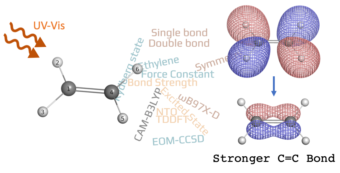
Equilibrium Geometries, Adiabatic Excitation Energies and Intrinsic C=C/C–H Bond Strengths of Ethylene in Lowest Singlet Excited States Described by TDDFT

Abstract

Seventeen singlet excited states of ethylene have been calculated via time-dependent density functional theory (TDDFT) with the CAM-B3LYP functional and the geometries of 11 excited states were optimized successfully. The local vibrational mode theory was employed to examine the intrinsic C=C/C–H bond strengths and their change upon excitation. The natural transition orbital (NTO) analysis was used to further analyze the C=C/C–H bond strength change in excited states versus the ground state. For the first time, three excited states including ${\pi }_y^{\prime }$ → 3s, ${\pi }_y^{\prime }$ → 3p${}_y$ and ${\pi }_y^{\prime }$ → 3p${}_z$ were identified with stronger C=C ethylene double bonds than in the ground state.

1. Introduction

Computational modeling of excited states is nowadays gaining more and more attention due to its increasing application in photochemistry and the rapid development of accurate and affordable computational methods [1,2,3,4,5,6]. While chemistry is majorly about the breaking/formation of chemical bonds, an important topic in modeling excited states is to analyze the chemical bonding of molecules in excited states.

The earliest theoretical tool in this regard dates back to 1983 when Dick and Freund developed a Cohen-type bond order [7] and also applied Wiberg’s index [8] to excited-state organic molecules. In the past two decades, various methods have been proposed to analyze excited-state chemical bonding including (1) the time-dependent electron localization function (ELF) [9] providing the time-resolved monitoring of chemical bonding dynamics, (2) the parity function [10] based on the spin-traced one-particle density matrix, (3) the quantum theory of atoms in molecules (QTAIM) [11] with its derived interacting quantum atoms (IQA) energy partition scheme [12], (4) the density overlap region indicator (DORI) [13] and (5) the adaptive natural density partitioning (AdNDP) method [14]. However, none of these aforementioned methods can directly quantify whether a chemical bond in a molecule is strengthened or weakened when this molecule is excited to a different electronic state.

One may think it is trivial to investigate chemical bonding of excited states because molecules with higher electronic energies should have generally lower bond energies implying that an excited-state molecule will have weaker chemical bonds (with the exception of excimers [15]). However, one needs to be aware that such a simplified picture overlooks the different types of electronic excitations and the heterogeneity in the molecular charge distribution Therefore, to understand the chemical bond strength and its change caused by electronic excitation is non-trivial. A bond weakening effect in excited states has been discovered in cyclopropyl ketones [16], double-bond species [17], metal-ligand bonds [18] and ligands within a manganese-nitride complex [19]. Han and co-workers pioneered the investigation of the so-called excited state hydrogen bond between a chromophore and protic solvents. They found that these hydrogen bonds can be strengthened or weakened upon excitation [20,21,22] and characterized the strengthening/weakening effect by calculating the hydrogen bond binding energy between chromophore and solvent molecules or by the red-/blue-shift of the O–H bond vibrational frequency.

Inspired by these studies on the excited state hydrogen bonding, we fostered the idea to apply the local vibrational mode theory [23] to excited-state molecules in order to obtain the intrinsic bond strength. The local vibrational mode theory was first developed by Konkoli and Cremer in 1998 [24] and its major idea is to extract from normal vibrational modes the local counterparts in terms of individual internal coordinates. For example, the local vibrational mode of a chemical bond corresponds to the motion initiated by an infinitesimal change in that bond length followed by the relaxation of all other atoms in this molecule. This local stretching mode in terms of bond length can then be used to characterize the intrinsic strength of the bond via the corresponding local stretching force constant $k^a$ or frequency ${\omega }^a$ [23]. In the past decade, the local vibrational mode theory has been applied to investigate the chemical bonding including covalent bonds, metal-ligand bonds and non-covalent interactions of molecules and solids in the ground state [23]. However, it has not been exclusively applied to study the bonding properties in the excited states, although this is theoretically feasible, because to conduct the local mode analysis for either ground state or excited states of a molecule requires only the equilibrium geometry of a molecule and its second-order energy derivative matrix (Hessian).

In this pilot study, we applied the local vibrational mode theory to quantify the intrinsic bond strength in the ethylene molecule in its excited states. The reason why we chose ethylene as a model system is because it is a rather simple molecule with one C=C double bond and four C–H single bonds. In addition, there are plenty of theoretical studies on the excited states of this molecule [17,25,26,27] to be used as a reference. We aimed to answer the following questions through this work:

• Does bond strengthening exist for the excited states of ethylene?
• To what extent can the bond strengthening/weakening be for the excited states of ethylene?
• How can we rationalize and interpret the result of bond strength changes determined with the local mode analysis?

The paper is structured in the following way. First, the computational details are given. In Section 3, we present the vertical excitation energies, adiabatic excitation energies, local C=C/C–H stretching force constants of ethylene in its excited states. The natural transition orbitals (NTOs) of the electronic excitations are shown to rationalize the intrinsic bond strength of ethylene. Important findings are summarized in Section 4.

2. Computational Details

The geometry of ethylene was optimized using the coupled-cluster singles and doubles (CCSD) [28] method with Dunning’s aug-cc-pVDZ basis set [29,30]. The optimized structure was then used in time-dependent density functional theory (TDDFT) and equation-of-motion coupled-cluster singles and doubles (EOM-CCSD) [31] calculations with Dunning’s aug-cc-pVTZ basis set [29,30] to obtain the vertical excitation energies (VEEs) of the lowest 17 singlet excited states (by specifying 20 excited state roots to find). The natural transition orbitals (NTOs) [32] analysis implemented in the Multiwfn 3.7 package [33] was employed to determine the character of the excited states where each electronic excitation is transformed into one or two pairs of compact orbital representations.

Eight out of the 17 calculated VEEs were compared with the experimentally measured excitation energies, then the root mean square (rms) and the mean signed average (MSA) deviations were calculated as following.

$$rms=\sqrt{\frac{{\sum }_{i=1}^8{(VE{E}_{calc,i}-VE{E}_{exp,i})}^2}{8}}$$

(1)

$$MSA=\frac{{\sum }_{i=1}^8(VE{E}_{calc,i}-VE{E}_{exp,i})}{8}$$

(2)

Based on the performance of different methods in reproducing the experimental excitation energies, the density functional CAM-B3LYP [34] was chosen for the (TD)DFT calculations to obtain optimized geometries of the singlet excited states as well as of the ground state. Noteworthy is that no symmetry constraint was imposed during the geometry optimizations. The vibrational analysis based on analytic second-order energy derivatives of TDDFT [35,36] was then carried out to confirm that the optimized geometries were indeed local minima on the potential energy surfaces (PES). In addition, the NTO analysis was applied to each optimized excited-state geometry to reassure that it is staying on the desired excited-state PES.

All calculations of VEEs, optimized geometries, adiabatic excitation energies (AEEs), Hessian matrices and normal vibrational analyses were carried out with the Gaussian 16 package [37].

The intrinsic C=C and C–H bond strength quantified by their local stretching force constants $k^a$ was calculated with the standalone LModeA package [23,38] based on the Hessian matrices.

3. Results and Discussion

Before characterizing the bonding properties of ethylene in its excited states, we benchmarked several levels of theory in terms of VEEs against 8 experimental excitation energies [25,26] in order to find the optimal method for theoretical calculations. As most low-lying excited states of ethylene are Rydberg states, we tested several frequently used density functionals with long-range corrections including LC-$\omega$HPBE [39], $\omega$hPBE0 [40], $\omega$B97X-D [41], CAMh-B3LYP [40], CAM-B3LYP [34] and M06-2X [42] for TDDFT calculations. In addition, the EOM-CCSD theory which is believed to outperform TDDFT was considered in our benchmark.

As shown in Figure 1, most density functionals have comparable rms deviations below 0.4 eV while LC-$\omega$HPBE has both large rms and MSA deviations. Surprisingly, the EOM-CCSD has larger errors (rms = 0.57, MSA = 0.47 eV) than TDDFT in calculating VEEs for ethylene. Among the tested density functionals, three of them have rms deviations equal or less than 0.3 eV including $\omega$hPBE0 (0.31 eV), CAM-B3LYP (0.31 eV) and $\omega$B97X-D (0.27 eV). The latter two functionals have MSA deviations less than 0.1 eV. Based on this result, we chose the CAM-B3LYP functional for the remaining calculations although $\omega$B97X-D would have been the other ideal option.

We calculated 17 lowest singlet excited states of ethylene at the CAM-B3LYP/aug-cc-pVTZ level with their irreducible representations, assignment and vertical excitation energies collected in

Table 1. Summary of the lowest 17 singlet excited states of ethylene calculated at CAM-B3LYP/aug-cc-pVTZ level of theory.

No.	State	Assignment ${}^{\mathit{a}}$	VEE [exp.] ${}^{\mathit{b}}$	f ${}^{\mathit{d}}$	Optimized Geometry
					Symmetry	AEE ${}^{\mathit{c}}$
0	1 A${}_g$	Ground State	0.00	-	D${}_{2h}$	–
1	1 B${}_{3u}$	$\pi$ → 3s	6.86 [7.11] [25]	0.0695	D${}_2$	6.80
2	1 B${}_{1u}$	$\pi$ → ${\pi }^{*}$	7.34 [7.63] [25,48]	0.3421	n/a
3	1 B${}_{1g}$	$\pi$ → 3p${}_y$	7.47 [7.80] [25]	0.0000	n/a
4	1 B${}_{2g}$	$\pi$ → 3p${}_z$	7.53 [8.00] [48]	0.0000	D${}_2$	7.45
5	2 B${}_{1g}$	${\pi }_y^{\prime }$ → 3d${}_{xz}$ (${\pi }^{*}$)	8.01	0.0000	C${}_{2h}$	7.80
6	2 A${}_g$	$\pi$ → 3p${}_x$	8.36 [8.29] [25]	0.0000	D${}_2$	7.96
7	1 A${}_u$	$\pi$ → 4d${}_{yz}$	8.58	0.0000	D${}_{2h}$	8.52
8	2 B${}_{3u}$	$\pi$ → 3d${}_{z^2}$	8.72 [8.62] [25]	0.0043	D${}_2$	8.65
9	1 B${}_{3g}$	${\pi }_y^{\prime }$ → 3s	9.18	0.0000	C${}_{2v}$	8.69
10	2 B${}_{2g}$	${\pi }_z^{\prime }$ → 3d${}_{xz}$ (${\pi }^{*}$)	9.39	0.0000	n/a
11	3 B${}_{3u}$	$\pi$ → 4s	9.56	0.0188	D${}_2$	9.49
12	3 B${}_{1g}$	$\pi$ → 4p${}_y$	9.68 [9.34] [25]	0.0000	n/a
13	3 B${}_{2g}$	$\pi$ → 4p${}_z$	9.68	0.0000	n/a
14	2 B${}_{1u}$	$\pi$ → 4d${}_{xz}$ (30%), ${\pi }_y^{\prime }$ → 3p${}_y$ (70%)	9.72 [9.33] [25]	0.0617	C${}_{2h}$	9.33
15	1 B${}_{2u}$	${\pi }_y^{\prime }$ → 3p${}_z$	9.80	0.0839	D${}_{2h}$	9.18
16	4 B${}_{3u}$	$\pi$ → 3d${}_{x^2-y^2}$	9.95	0.2225	D${}_2$	9.85
17	3 B${}_{1u}$	$\pi$ → 4d${}_{xz}$ (70%), ${\pi }_y^{\prime }$ → 3p${}_y$ (30%)	9.99	0.0086	n/a

${}^a$ The character of electronic excitation is determined based on the natural transition orbitals (NTOs) analysis. The C=C bond axis is defined as the z direction while the x direction is defined to be perpendicular to the geometrical plane of ethylene (see Figure 2). ${}^b$ Vertical excitation energies in eV. Experimental excitation energy is recorded in brackets. ${}^c$ Adiabatic excitation energies in eV. ${}^d$ Oscillator strength.

. In order to quantify the intrinsic bond strength of ethylene in its excited states with the local vibrational mode theory, it is required to first optimize the ethylene geometry accordingly. The equilibrium geometries of 11 among the 17 excited states were successfully determined while the remaining 6 states could not be optimized due to two possible reasons: (1) the target excited-state PES has no local minima (with vanishing gradients) as it may form a crossing seam or canonical intersection with another electronic state; (2) the geometry optimizer fails to stay on the desired excited-state PES and crosses to the PES of another undesired electronic state [43].

The C=C/C–H bond lengths, point group and adiabatic excitation energies of the optimized geometries of ethylene in different excited states are complied in Table 1 and

Table 2. Bond length r (Å) and local stretching force constant $k^a$ (mdyn/Å) for C=C/C–H bonds in ethylene in different excited-state equilibrium geometries calculated at CAM-B3LYP/aug-cc-pVTZ level.

No.	rCC	${\mathbf{k}}_{\mathbf{CC}}^{\mathbf{a}}$	BSO${}_{\mathbf{CC}}$	rCH	${\mathbf{k}}_{\mathbf{CH}}^{\mathbf{a}}$
0	1.3193	10.022	2.0	1.0817	5.575
1	1.3828	5.785	1.3	1.0852	5.412
4	1.3863	5.416	1.2	1.0868	2.462
5	1.3700	5.325	1.2	1.1218 (C1H2,C4H5)	4.096
				1.0843 (C1H3,C4H6)	4.960
6	1.3558	7.254	1.6	1.0860	5.461
7	1.4057	7.223	1.6	1.0798	5.648
8	1.3864	5.228	1.2	1.0858	5.301
9	1.2632	11.701	2.2	1.0980 (C1H2,C1H3)	3.917
				1.1528 (C4H5,C4H6)	1.579
11	1.3991	5.653	1.3	1.0973	3.979
14	1.2577	11.348	2.2	1.0990 (C1H2,C4H5)	4.219
				1.1659 (C1H3,C4H6)	2.666
15	1.2598	12.686	2.4	1.1313	2.864
16	1.3855	6.014	1.3	1.0812	5.583
Ethane	1.5214	4.256	1.0	1.0898	5.220
Ethyne	1.1911	17.992	3.0	1.0619	6.416

, while the Cartesian coordinates are available in the Supplementary Materials. Due to the pseudo-Jahn–Teller effect [44], there exists some connection between the symmetry of the excited state and the point group of its equilibrium geometry. Among the 11 states investigated in this work, the B${}_{3u}$ states always leads to D${}_2$-symmetry non-planar structures. The A${}_g$ states leads to either D${}_2$ or D${}_{2h}$ structures. The C${}_{2h}$-symmetry structures can arise from the B${}_{1u}$ and B${}_{1g}$ states. The B${}_{3g}$ state can lead to very unique C${}_{2v}$ structure where two carbon atoms are no longer equivalent.

By employing the local vibrational mode theory, the local stretching force constants $k^a$ were determined for C=C and C–H bonds of these optimized geometries of ethylene and the results are collected in Table 2.

Figure 2, Figure 3 and Figure 4 show the distribution of the local stretching force constants as intrinsic bond strength measure for C=C and C–H bonds of ethylene in its excited-state equilibrium geometries. For both types of bonds, the bond strength is overall weakened as expected for the 11 excited states investigated in this work. However, three and two excited states exhibit stronger C=C and C–H bonds than ground state (S${}_0$) respectively.

By correlating the local stretching force constant $k^a$ and bond length r for C=C bonds as shown in Figure 2, we found a strong linear correlation for 9 out of 11 excited states with the coefficient of determination (R${}^2$) of 0.966. The generalized Badger’s rule [45] implying that shorter bonds are stronger is valid. However, the ethane C–C single bond is out of trend in this $k^a$-r relationship, which is in line with the fact that single and double CC bonds have different bonding nature.

In order to translate the local stretching force constant $k^a$ for C=C bonds of ethylene into a more chemically intuitive quantity, we propose to use the bond strength order (BSO) [46] in reminiscence of Pauling’s bond order (BO) [47]. As shown in Figure 3, we first used the local stretching force constants of ethane C–C, ethylene C=C and ethyne C≡C bonds to define the reference BSO values of 1.0, 2.0 and 3.0 respectively. Then a cubic function between BSO and $k^a$ was used to fit these three points and the origin. We found the C=C bonds of most excited states have a BSO of 1.2–1.3, which is close to the C–C bond strength in ethane. Two excited states have their C=C bond BSOs of 1.6. The strengthened C=C bonds for 3 excited states have BSOs of 2.2–2.4, which are smaller than the bond strength of ethyne C≡C bond.

In addition, Figure 4 shows the relationship between $k^a$ and r for C–H bonds of ethylene and we observed a weaker correlation between these two quantities (R${}^2$ = 0.902).

In order to better understand the variation in the intrinsic C=C/C–H bond strength of ethylene in excited states, we calculated the natural transition orbitals (NTOs) [32] of all 17 singlet excited states investigated in this work. The underlying idea of the NTO analysis is a unitary transformation of the occupied and virtual orbitals with no change towards the transition density. By correlating transformed occupied/virtual orbitals (i.e., NTOs) into pairs, one can easily obtain the straightforward physical picture of the excitation of “particle” into the empty “hole”. Figure 5, Figure 6 and Figure 7 illustrate the NTO diagrams of the 11 excited states whose equilibrium geometries and bonding properties are investigated in this work. The NTO diagrams for the remaining 6 singlet excited states can be found in the Supplementary Materials.

Most of the 11 singlet excited states of ethylene investigated in this work have the electronic excitation from the $\pi$ bonding orbital, except S${}_5$, S${}_9$, S${}_{14}$ and S${}_{15}$. The “particle” NTO of these 4 excited states is ${\pi }_y^{\prime }$ orbital which consists of the 2p${}_y$ atomic orbitals of C and the s orbitals of H. One interesting observation is that S${}_9$, S${}_{14}$ and S${}_{15}$ have C=C bonds stronger than the ground state (S${}_0$) ethylene, while the S${}_5$ state has weaker C=C bond. The ${\pi }_y^{\prime }$ orbital has a similar shape as the ${\pi }^{*}$ anti-bonding orbital except its orientation and therefore this orbital has anti-bonding character. When the electron is excited from ${\pi }_y^{\prime }$ orbital, the depletion in this anti-bonding orbital can lead to stronger C=C bonds for S${}_9$, S${}_{14}$ and S${}_{15}$. However, in the case of the S${}_5$ state the electron is excited to the real ${\pi }^{*}$ anti-bonding orbital from the ${\pi }_y^{\prime }$ anti-bonding orbital, thus the C=C bond is weakened compared to the ground state. Noteworthy is that the C=C bond of S${}_{15}$ state is slightly stronger than for the S${}_9$ and S${}_{14}$ states. Unlike S${}_9$ and S${}_{14}$, the “hole” NTO of S${}_{15}$ has some ${\sigma }^{*}$ anti-bonding character due to the presence of a node between two carbon atoms, it is not quite clear why such excitation could lead to the strongest C=C bond at this moment.

For those excited states whose particle NTO is the $\pi$ bonding orbital, the C=C bonds are weakened to different extent. The S${}_6$ and S${}_7$ are relatively stronger than others. In the case of S${}_6$, the electron is excited from the 2p${}_x$ $\pi$ bonding orbital into 3p${}_x$ $\pi$ bonding orbital, however, the C=C bond is weakened.

For the C–H bonds of ethylene in its excited states, the S${}_{16}$ state has almost the same C–H strength as the ground state and only S${}_7$ has a marginally stronger C–H bond. The NTO diagrams for the S${}_7$ state show that the electron is excited from the $\pi$ bonding orbital into the 4d${}_{yz}$ orbital which contains 4 $\sigma$(C–H) bonding orbitals and this explains why the C–H bonds in S${}_7$ state are strengthened.

When the electron is excited from the ${\pi }_y^{\prime }$ orbital in the cases of S${}_5$, S${}_9$, S${}_{14}$ and S${}_{15}$, the C–H bonds are unanimously weakened because their particle NTO consists of 4 $\sigma$(C–H) bonding orbitals and electron depletion from this orbital can lead to weaker C–H bonds. The C–H bonds in S${}_{15}$ state are greatly weakened and this can be related to the existence of the anti-bonding nodes of the 3p${}_z$ orbital as shown in Figure 6. Interesting is that the S${}_4$ state has also quite weak C–H bonds (see Figure 4). Its hole NTO is the same as the hole NTO of S${}_{15}$ where 4 anti-bonding nodes exist for the C–H bonds.

Due to symmetry, not all C–H bonds are equivalent in ethylene for some excited states. S${}_5$, S${}_9$ and S${}_{14}$ have two sets of C–H bonds and the difference in the local stretching force constant between two sets is 0.86, 2.34 and 1.55 mdyn/Å, respectively. In the case of S${}_9$ where the electron is excited from ${\pi }_y^{\prime }$ orbital to 3s orbital leading to unbalanced charge distribution of the ethylene molecule, the C–H bonds at one side have their local stretching force constant being 1.6 mdyn/Å as the lowest value among all C–H bonds.

The S${}_1$ and S${}_{11}$ states have very similar NTO character in their excitations as the former has the 3s orbital as the hole NTO and the latter has 4s orbital as the hole NTO while their particle NTO is the same. Both states have weakened C–H bond strength compared to the ground states. However, the S${}_{11}$ state has its C–H bonds weakened to a much larger extent and this can be related to its more pronounced C–H anti-bonding character in the hole orbital as shown in Figure 5.

4. Conclusions

In this work, we calculated the 17 lowest singlet excited states of ethylene in gas phase with TDDFT and analyzed the C=C/C–H bonding properties by combining the local vibrational mode theory and natural bond orbitals (NTOs). This led to the following important findings:

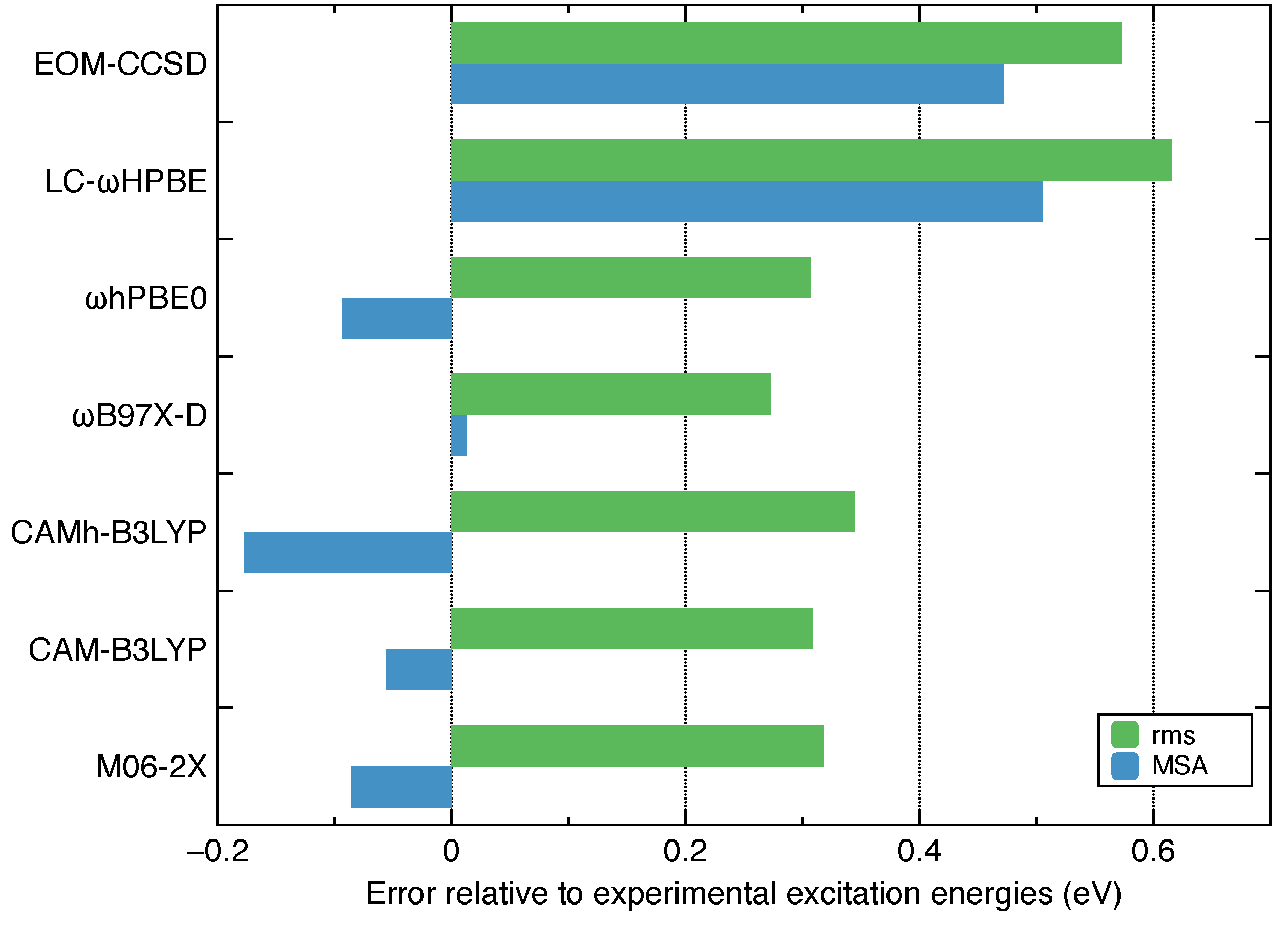
• Among the several commonly used density functionals for describing the Rydberg states, $\omega$B97X-D, CAM-B3LYP and $\omega$hPBE0 give relatively low rms deviations (∼0.3 eV) against the experimental excitation energies for ethylene.
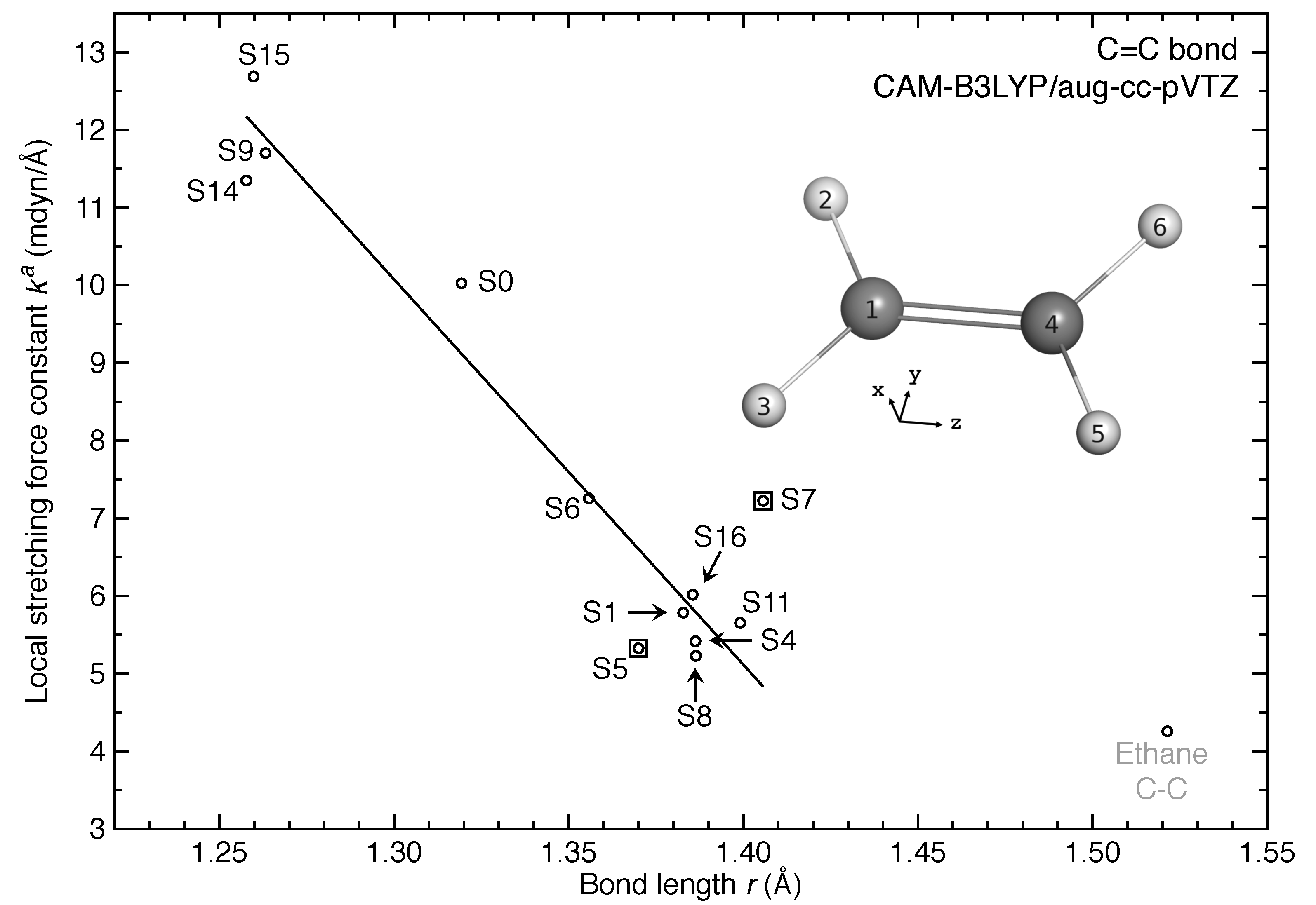
• The equilibrium geometries for 11 out of 17 excited states of ethylene were successfully modeled at the CAM-B3LYP/aug-cc-pVTZ level. Six of them are twisted in contrast to the planar ground-state structure.
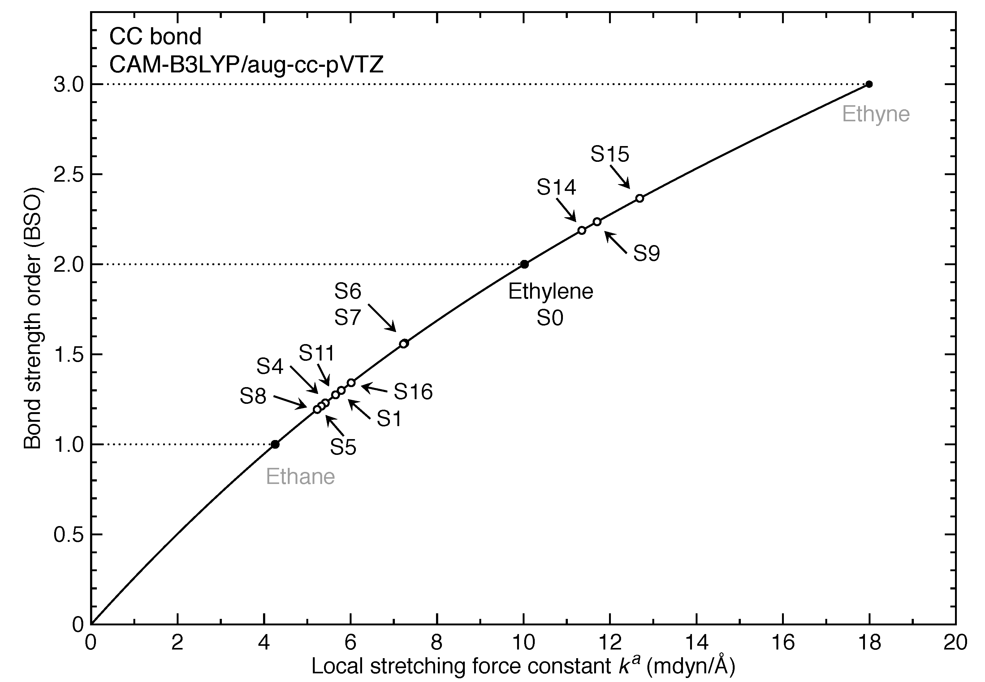
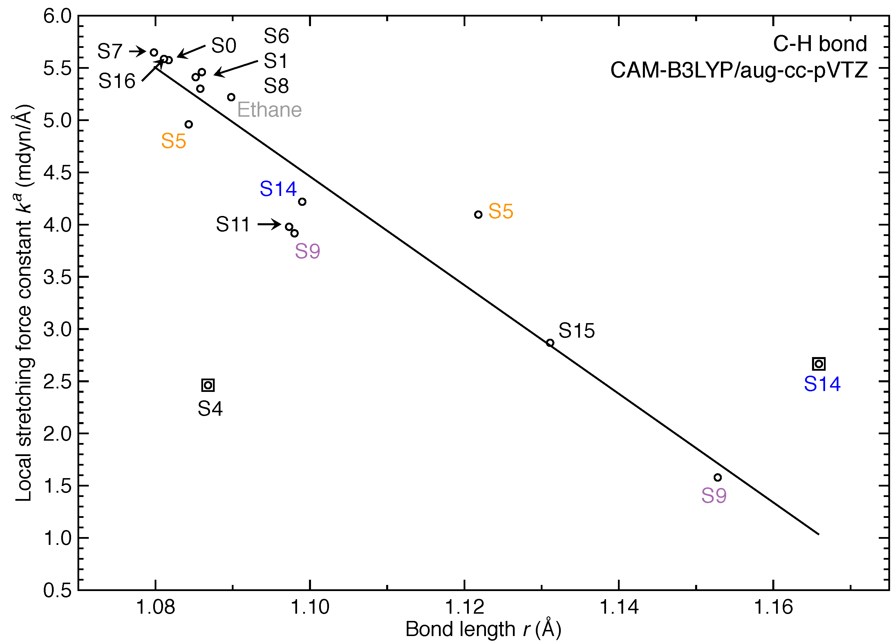
• For the first time, the local vibrational mode theory has been applied to molecules in excited states to characterize the intrinsic bond strength which can be directly compared with the ground-state counterpart. In this study on ethylene, the majority of the 11 excited states with optimized geometries exhibit weakened C=C/C–H bonds as characterized by the local stretching force constant $k^a$, which is consistent with the assumption that a molecule in its excited states with higher electronic energy has in general smaller bond (dissociation) energies. However, the results from the local mode analysis show that 3 excited states have stronger C=C bonds with BSO values of 2.4, which almost reaches the midpoint between ethylene C=C (BSO = 2.0) and ethyne C≡C (BSO = 3.0). Meanwhile, 2 excited states show only marginally stronger C–H bond strength the ground state. Overall, the local stretching force constants for these 11 excited states of ethylene show a larger range of variation for the C=C bond compared to the ground state (variation of −48 % to +27 %) than for C–H bonds (variation of −72 % to +1 %). This leads to the important conclusion that the C=C bond of ethylene is more tunable by electronic excitation, while this does not hold for the C–H bond.
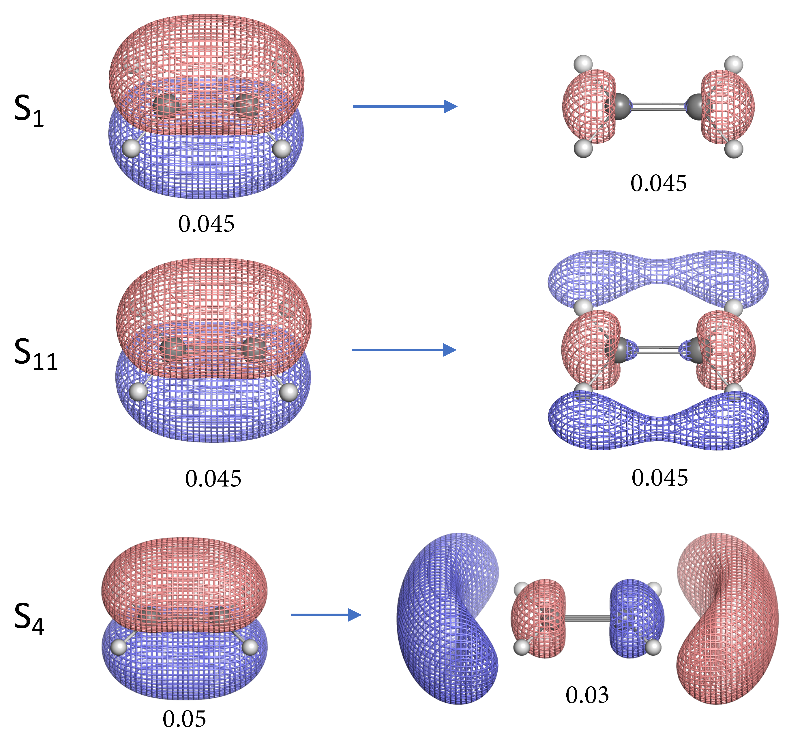
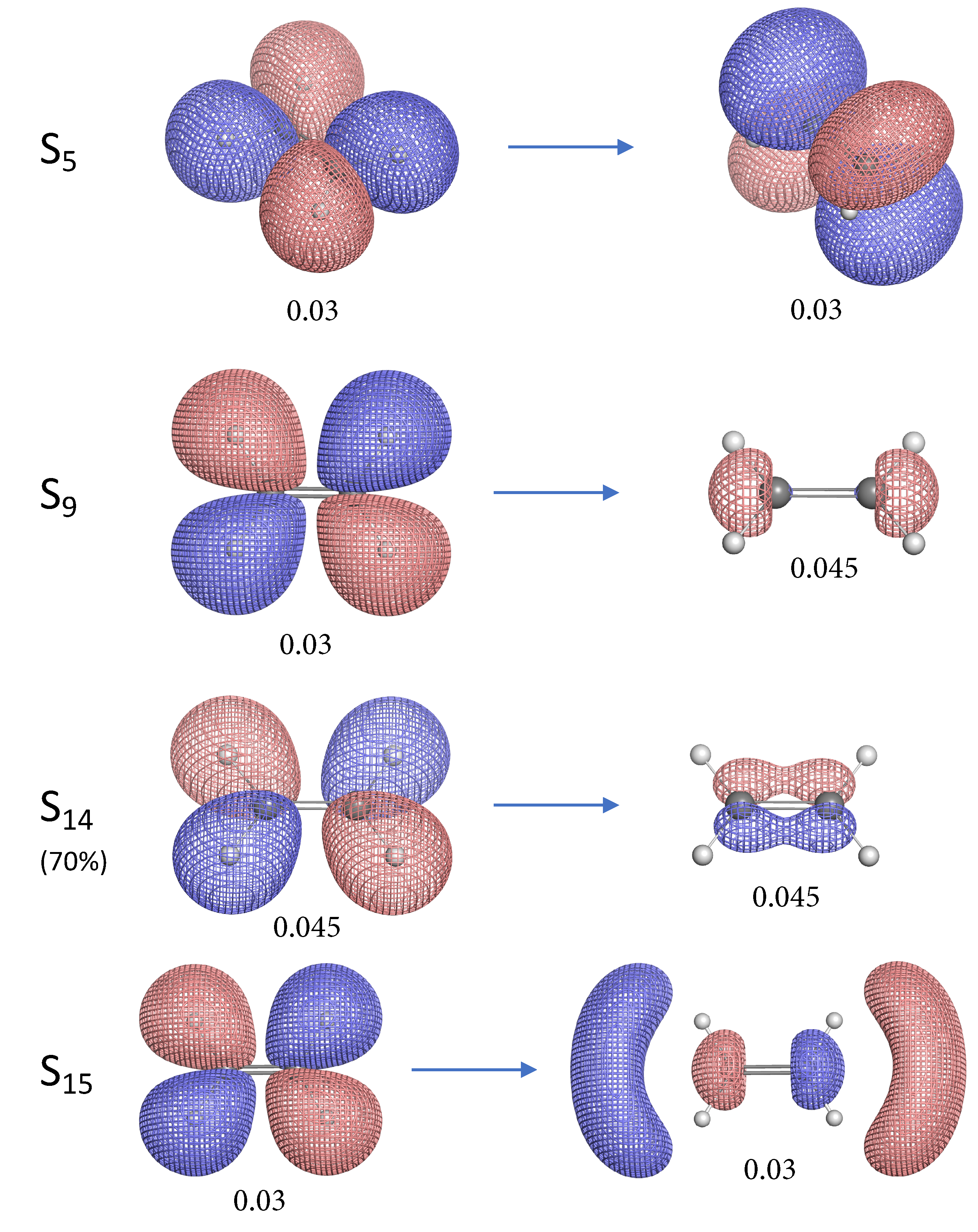
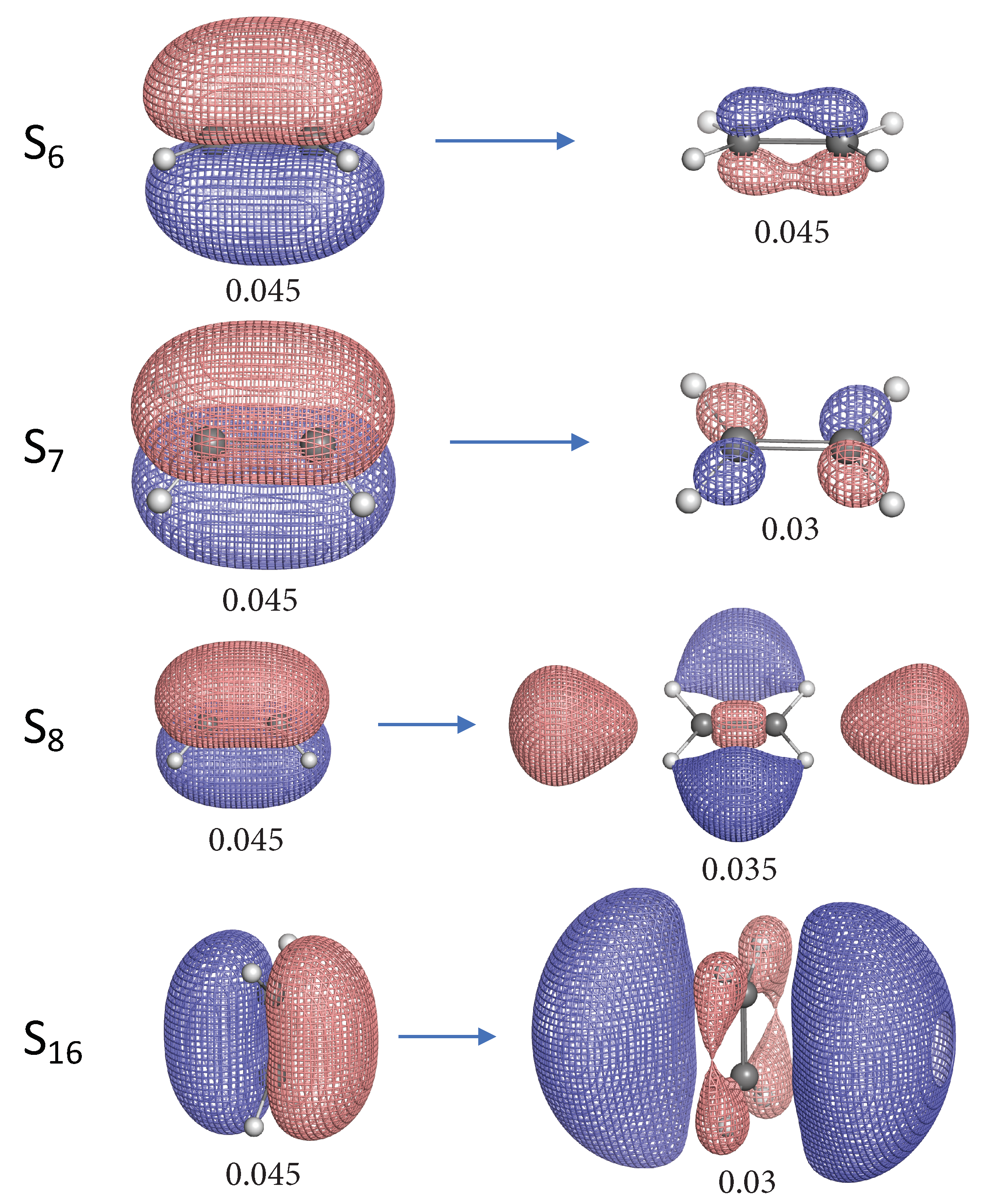
• The NTO analysis plays an important role in helping interpret the result of local stretching force constants for C=C/C–H bonds of ethylenes in excited states.
  • When the particle NTO is the $\pi$ bonding orbital, the C=C bond is always weakened in terms of local stretching force constant.
  • When the particle NTO is the ${\pi }_y^{\prime }$ orbital arising from the $\sigma$-backbone of ethylene, the C=C bond is in general strengthened except when the hole NTO is the ${\pi }^{*}$ anti-bonding orbital. Surprisingly, when the hole NTO orbital is 3p${}_z$ the C=C bond is the strongest and this hole NTO has ${\sigma }^{*}$(C=C) anti-bonding character.
  • The excited state leading to slightly increased C–H bond strength has its hole NTO as 4d${}_{yz}$ which consists of 4 C–H bonding orbitals.
  • When the hole NTO has significant C–H anti-bonding character, the C–H bonds are greatly weakened.
• Computational modeling of molecular excited states is generally more challenging than for the ground state. Therefore, we used ethylene as a simple theoretical model system to provide the proof of concept that fine-tuning chemical bond strength via electronic excitation is feasible, although the calculations performed in this work can be further improved by more advanced wavefunction-based correlation methods other than TDDFT [5,27]. It is also possible to find the equilibrium geometries of more excited states with dedicated algorithms [43], which we will test in the future.

We hope our work will spur a similar interest in exploring chemical bonding properties of excited states among both experimental and theoretical chemists.

References

1. Mai, S.; González, L. Molecular Photochemistry: Recent Developments in Theory. Angew. Chem. Int. Ed. 2020, 59, 16832–16846. [Google Scholar] [CrossRef]
2. Hait, D.; Head-Gordon, M. Excited State Orbital Optimization via Minimizing the Square of the Gradient: General Approach and Application to Singly and Doubly Excited States via Density Functional Theory. J. Chem. Theory Comput. 2020, 16, 1699–1710. [Google Scholar] [CrossRef]
3. Mewes, S.A.; Dreuw, A. Density-based descriptors and exciton analyses for visualizing and understanding the electronic structure of excited states. Phys. Chem. Chem. Phys. 2019, 21, 2843–2856. [Google Scholar] [CrossRef]
4. Liu, Y.; Kilby, P.; Frankcombe, T.J.; Schmidt, T.W. Electronic transitions of molecules: Vibrating Lewis structures. Chem. Sci. 2019, 10, 6809–6814. [Google Scholar] [CrossRef] [PubMed]
5. Loos, P.F.; Scemama, A.; Blondel, A.; Garniron, Y.; Caffarel, M.; Jacquemin, D. A Mountaineering Strategy to Excited States: Highly Accurate Reference Energies and Benchmarks. J. Chem. Theory Comput. 2018, 14, 4360–4379. [Google Scholar] [CrossRef] [PubMed]
6. González, L.; Escudero, D.; Serrano-Andrés, L. Progress and Challenges in the Calculation of Electronic Excited States. ChemPhysChem 2012, 13, 28–51. [Google Scholar] [CrossRef] [PubMed]
7. Dick, B.; Freund, H.J. Analysis of Bonding Properties in Molecular Ground and Excited States by a Cohen-Type Bond Order. Int. J. Quantum Chem. 1983, 24, 747–765. [Google Scholar] [CrossRef] [Green Version]
8. Wiberg, K. Application of the Pople-Santry-Segal CNDO Method to the Cyclopropylcarbinyl and Cyclobutyl Cation and to Bicyclobutane. Tetrahedron 1968, 24, 1083–1096. [Google Scholar] [CrossRef]
9. Burnus, T.; Marques, M.A.L.; Gross, E.K.U. Time-Dependent Electron Localization Function. Phys. Rev. A 2005, 71, 010501. [Google Scholar] [CrossRef] [Green Version]
10. Kadantsev, E.S.; Schmider, H.L. Analysis of Chemical Bonding in Electronic Excited States Using Parity Function. Int. J. Quantum Chem. 2007, 108, 1–14. [Google Scholar] [CrossRef]
11. Ferro-Costas, D.; Pendás, Á.M.; González, L.; Mosquera, R.A. Beyond the Molecular Orbital Conception of Electronically Excited States Through the Quantum Theory of Atoms in Molecules. Phys. Chem. Chem. Phys. 2014, 16, 9249–9258. [Google Scholar] [CrossRef] [PubMed] [Green Version]
12. Jara-Cortés, J.; Guevara-Vela, J.M.; Pendás, Á.M.; Hernández-Trujillo, J. Chemical Bonding in Excited States: Energy Transfer and Charge Redistribution From a Real Space Perspective. J. Comput. Chem. 2017, 38, 957–970. [Google Scholar] [CrossRef] [PubMed]
13. Vannay, L.; Brémond, E.; de Silva, P.; Corminboeuf, C. Visualizing and Quantifying Interactions in the Excited State. Chem. Eur. J. 2016, 22, 18442–18449. [Google Scholar] [CrossRef] [PubMed]
14. Tkachenko, N.V.; Boldyrev, A.I. Chemical Bonding Analysis of Excited States Using the Adaptive Natural Density Partitioning Method. Phys. Chem. Chem. Phys. 2019, 21, 9590–9596. [Google Scholar] [CrossRef]
15. Birks, J.B. Excimers. Rep. Prog. Phys. 1975, 38, 903–974. [Google Scholar] [CrossRef]
16. Zimmerman, H.E.; Hixson, S.S.; McBride, E.F. Excited State Bond Weakening in Photochemical Rearrangements of Cyclopropyl Ketones. Exploratory and Mechanistic Organic Photochemistry. XLVIII. J. Am. Chem. Soc. 1970, 92, 2000–2015. [Google Scholar] [CrossRef]
17. Badenhoop, J.K.; Scheiner, S. Characterization of Ground and Excited Electronic State Deprotonation Energies of Systems Containing Double Bonds Using Natural Bond Orbital Analysis. J. Chem. Phys. 1996, 105, 4675–4691. [Google Scholar] [CrossRef] [Green Version]
18. Zink, J.I. Photo-Induced Metal-Ligand Bond Weakening, Potential Surfaces, and Spectra. Coord. Chem. Rev. 2001, 211, 69–96. [Google Scholar] [CrossRef]
19. Loose, F.; Wang, D.; Tian, L.; Scholes, G.D.; Knowles, R.R.; Chirik, P.J. Evaluation of Excited State Bond Weakening for Ammonia Synthesis from a Manganese Nitride: Stepwise Proton Coupled Electron Transfer is Preferred over Hydrogen Atom Transfer. Chem. Commun. 2019, 55, 5595–5598. [Google Scholar] [CrossRef]
20. Zhao, G.J.; Han, K.L. Hydrogen Bonding in the Electronic Excited State. Acc. Chem. Res. 2012, 45, 404–413. [Google Scholar] [CrossRef]
21. Chu, T.S.; Liu, B.T. Establishing New Mechanisms with Triplet and Singlet Excited-State Hydrogen Bonding Roles in Photoinduced Liquid Dynamics. Int. Rev. Phys. Chem. 2016, 35, 187–208. [Google Scholar] [CrossRef]
22. Chu, T.S.; Xu, J. Photoinduced Hydrogen-Bonding Dynamics. J. Mol. Model. 2016, 22, 200. [Google Scholar] [CrossRef] [PubMed]
23. Kraka, E.; Zou, W.; Tao, Y. Decoding Chemical Information from Vibrational Spectroscopy Data—Local Vibrational Mode Theory. WIREs Comput. Mol. Sci. 2020, 10, e1480. [Google Scholar] [CrossRef]
24. Konkoli, Z.; Cremer, D. A New Way of Analyzing Vibrational Spectra. I. Derivation of Adiabatic Internal Modes. Int. J. Quantum Chem. 1998, 67, 1–9. [Google Scholar] [CrossRef]
25. Wiberg, K.B.; Hadad, C.M.; Foresman, J.B.; Chupka, W.A. Electronically Excited States of Ethylene. J. Phys. Chem. 1992, 96, 10756–10768. [Google Scholar] [CrossRef]
26. Head-Gordon, M.; Rico, R.J.; Oumi, M.; Lee, T.J. A Doubles Correction to Electronic Excited States from Configuration Interaction in the Space of Single Substitutions. Chem. Phys. Lett. 1994, 219, 21–29. [Google Scholar] [CrossRef] [Green Version]
27. Feller, D.; Peterson, K.A.; Davidson, E.R. A Systematic Approach to Vertically Excited States of Ethylene Using Configuration Interaction and Coupled Cluster Techniques. J. Chem. Phys. 2014, 141, 104302. [Google Scholar] [CrossRef]
28. Scuseria, G.E.; Janssen, C.L.; Schaefer, H.F. An Efficient Reformulation of the Closed-Shell Coupled Cluster Single and Double Excitation (CCSD) Equations. J. Chem. Phys. 1988, 89, 7382–7387. [Google Scholar] [CrossRef]
29. Dunning, T.H. Gaussian Basis Sets for Use in Correlated Molecular Calculations. I. The Atoms Boron Through Neon and Hydrogen. J. Chem. Phys. 1989, 90, 1007–1023. [Google Scholar] [CrossRef]
30. Kendall, R.A.; Dunning, T.H.; Harrison, R.J. Electron Affinities of the First-Row Atoms Revisited. Systematic Basis Sets and Wave Functions. J. Chem. Phys. 1992, 96, 6796–6806. [Google Scholar] [CrossRef] [Green Version]
31. Stanton, J.F.; Bartlett, R.J. The Equation of Motion Coupled-Cluster Method. A Systematic Biorthogonal Approach to Molecular Excitation Energies, Transition Probabilities, and Excited State Properties. J. Chem. Phys. 1993, 98, 7029–7039. [Google Scholar] [CrossRef]
32. Martin, R.L. Natural Transition Orbitals. J. Chem. Phys. 2003, 118, 4775–4777. [Google Scholar] [CrossRef]
33. Lu, T.; Chen, F. Multiwfn: A Multifunctional Wavefunction Analyzer. J. Comput. Chem. 2011, 33, 580–592. [Google Scholar] [CrossRef]
34. Yanai, T.; Tew, D.P.; Handy, N.C. A New Hybrid Exchange-Correlation Functional Using the Coulomb-Attenuating Method (CAM-B3LYP). Chem. Phys. Lett. 2004, 393, 51–57. [Google Scholar] [CrossRef] [Green Version]
35. Liu, J.; Liang, W. Analytical Hessian of Electronic Excited states in Time-Dependent Density Functional Theory with Tamm-Dancoff Approximation. J. Chem. Phys. 2011, 135, 014113. [Google Scholar] [CrossRef]
36. Liu, J.; Liang, W. Analytical Approach for the Excited-State Hessian in Time-Dependent Density Functional Theory: Formalism, Implementation, and Performance. J. Chem. Phys. 2011, 135, 184111. [Google Scholar] [CrossRef]
37. Frisch, M.J.; Trucks, G.W.; Schlegel, H.B.; Scuseria, G.E.; Robb, M.A.; Cheeseman, J.R.; Scalmani, G.; Barone, V.; Petersson, G.A.; Nakatsuji, H.; et al. Gaussian 16 Revision B.01; Gaussian Inc.: Wallingford, CT, USA, 2016. [Google Scholar]
38. Zou, W.; Tao, Y.; Freindorf, M.; Makos, M.; Verma, N.; Kraka, E. LMODEA2020; Southern Methodist University: Dallas, TX, USA, 2020. [Google Scholar]
39. Henderson, T.M.; Izmaylov, A.F.; Scalmani, G.; Scuseria, G.E. Can Short-Range Hybrids Describe Long-Range-Dependent Properties? J. Chem. Phys. 2009, 131, 044108. [Google Scholar] [CrossRef]
40. Shao, Y.; Mei, Y.; Sundholm, D.; Kaila, V.R.I. Benchmarking the Performance of Time-Dependent Density Functional Theory Methods on Biochromophores. J. Chem. Theory Comput. 2019, 16, 587–600. [Google Scholar] [CrossRef] [Green Version]
41. Chai, J.D.; Head-Gordon, M. Long-Range Corrected Hybrid Density Functionals with Damped Atom-Atom Dispersion Corrections. Phys. Chem. Chem. Phys. 2008, 10, 6615. [Google Scholar] [CrossRef] [Green Version]
42. Zhao, Y.; Truhlar, D.G. The M06 Suite of Density Functionals for Main Group Thermochemistry, Thermochemical Kinetics, Noncovalent Interactions, Excited States, and Transition Elements: Two New Functionals and Systematic Testing of Four M06-Class Functionals and 12 Other Functionals. Theor. Chem. Acc. 2007, 120, 215–241. [Google Scholar]
43. García, J.S.; Boggio-Pasqua, M.; Ciofini, I.; Campetella, M. Excited State Tracking During the Relaxation of Coordination Compounds. J. Comput. Chem. 2019, 40, 1420–1428. [Google Scholar] [CrossRef] [Green Version]
44. Bersuker, I. The Jahn-Teller Effect; Cambridge University Press: Cambridge, UK, 2006. [Google Scholar]
45. Kraka, E.; Larsson, J.A.; Cremer, D. Generalization of the Badger Rule Based on the Use of Adiabatic Vibrational Modes. In Computational Spectroscopy; Grunenberg, J., Ed.; Wiley: New York, NY, USA, 2010; pp. 105–149. [Google Scholar]
46. Zou, W.; Cremer, D. C2 in a Box: Determining its Intrinsic Bond Strength for the X1Σ+g Ground State. Chem. Eur. J. 2016, 22, 4087–4097. [Google Scholar] [CrossRef] [PubMed]
47. Pauling, L. Atomic Radii and Interatomic Distances in Metals. J. Am. Chem. Soc. 1947, 69, 542–553. [Google Scholar] [CrossRef]
48. Leang, S.S.; Zahariev, F.; Gordon, M.S. Benchmarking the Performance of Time-Dependent Density Functional Methods. J. Chem. Phys. 2012, 136, 104101. [Google Scholar] [CrossRef] [PubMed] [Green Version]
Figure 1. Root mean square (rms) and mean signed average (MSA) differences (in eV) between vertical excitation energies calculated theoretically and experimentally measured excitation energies for the ethylene molecule. Eight singlet excited states are included in comparison.
Symmetry 12 01545 g001
Figure 2. Relationship between local stretching force constant k a and bond length r for C=C bond of ethylene in different excited-state equilibrium geometries. Linear fitting was employed for 10 data points with R 2 = 0.966 while S5 and S7 identified as outliers were excluded for fitting.
Symmetry 12 01545 g002
Figure 3. Distribution of bond strength order (BSO) of C=C bond in ethylene in different excited-state equilibrium geometries. BSO is defined as a cubic function ( y = 0.00014718 x 3 0.0082412 x 2 + 0.26737 x ) of the local stretching force constant for CC bonds where the ethane C–C, ethylene C=C and ethyne C≡C bonds takes the BSO values of 1.0, 2.0 and 3.0, respectively as references.
Symmetry 12 01545 g003
Figure 4. Relationship between local stretching force constant k a and bond length r for C–H bond of ethylene in different excited-state equilibrium geometries. Linear fitting was employed for 14 data points with R 2 = 0.902 while S4 and one S14 identified as outliers were excluded for fitting. In addition, the C–H bond of ethane molecule was included in the linear fitting.
Symmetry 12 01545 g004
Figure 5. Natural transition orbital (NTO) pairs illustrating the singlet excited states of ethylene. The label S n for each excited state corresponds to the first column of Table 1. The left and right NTO diagrams shown as mesh isosurfaces depict the excited particle (occupied) and empty hole (unoccupied) respectively. The red and blue colors are chosen arbitrarily to indicate two different phases. Below each isosurface is the corresponding isovalue in atomic units (a.u.). Each NTO pair accounts for more than 90% contribution to the target electronic excitation unless otherwise specified.
Symmetry 12 01545 g005
Figure 6. Continued from Figure 5.
Symmetry 12 01545 g006
Figure 7. Continued from Figure 6.
Symmetry 12 01545 g007