Author Contributions
Conceptualization, M.H., M.U. and W.W.; methodology, M.H.; M.U., software, M.H., M.U.; validation, M.H., M.U.; formal analysis, M.H., M.U.; investigation, M.H.; M.U., writing—original draft preparation, M.H., M.U.; writing—review and editing, O.M.F.; visualization, I.K.; supervision, M.U., W.W.; project administration, I.K., O.M.F.; funding acquisition, O.M.F. All authors have read and agreed to the published version of the manuscript.
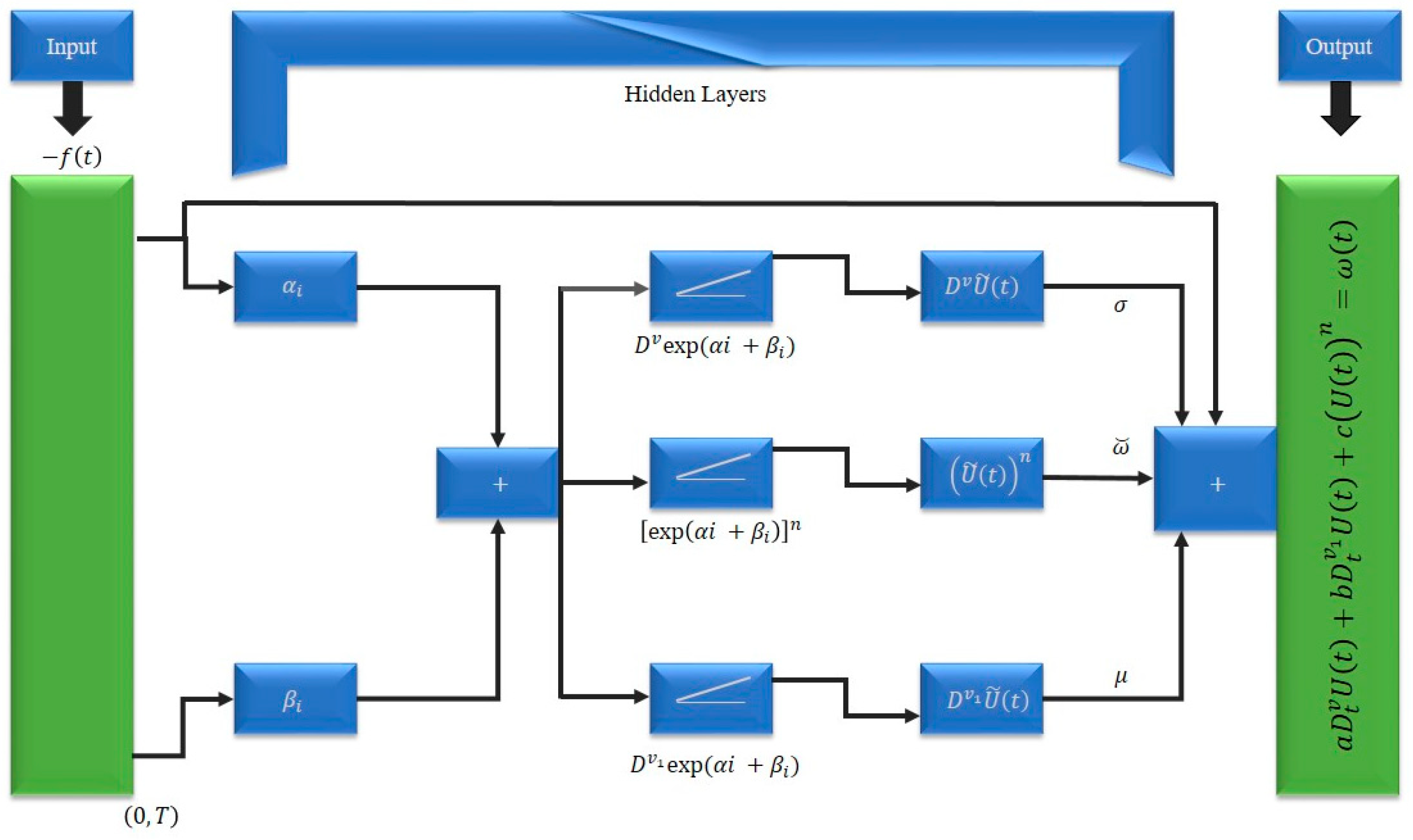
Figure 1.
The Bagley–Torvik (BT) equation arise in FDE-NNs architecture.
Figure 1.
The Bagley–Torvik (BT) equation arise in FDE-NNs architecture.
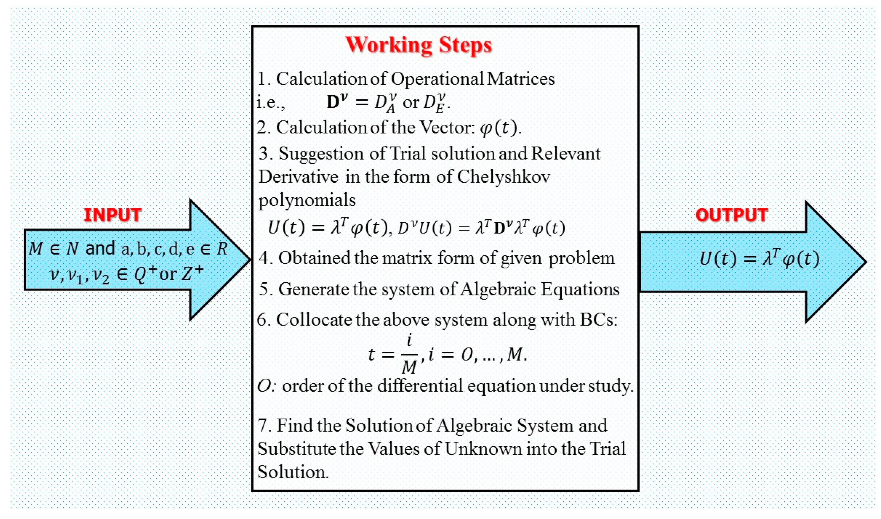
Figure 2.
The flow chart of the algorithm.
Figure 2.
The flow chart of the algorithm.
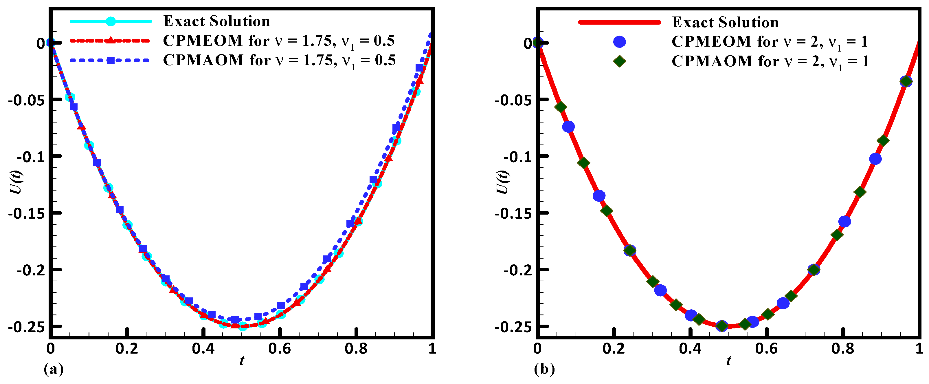
Figure 3.
The graphical representation (Problem 1) exact solution, Chelyshkov polynomial method (CPM) solution via and CPM soliton via . (a). Comparison for fractional order derivatives. (b). Comparison for integer order derivative.
Figure 3.
The graphical representation (Problem 1) exact solution, Chelyshkov polynomial method (CPM) solution via and CPM soliton via . (a). Comparison for fractional order derivatives. (b). Comparison for integer order derivative.
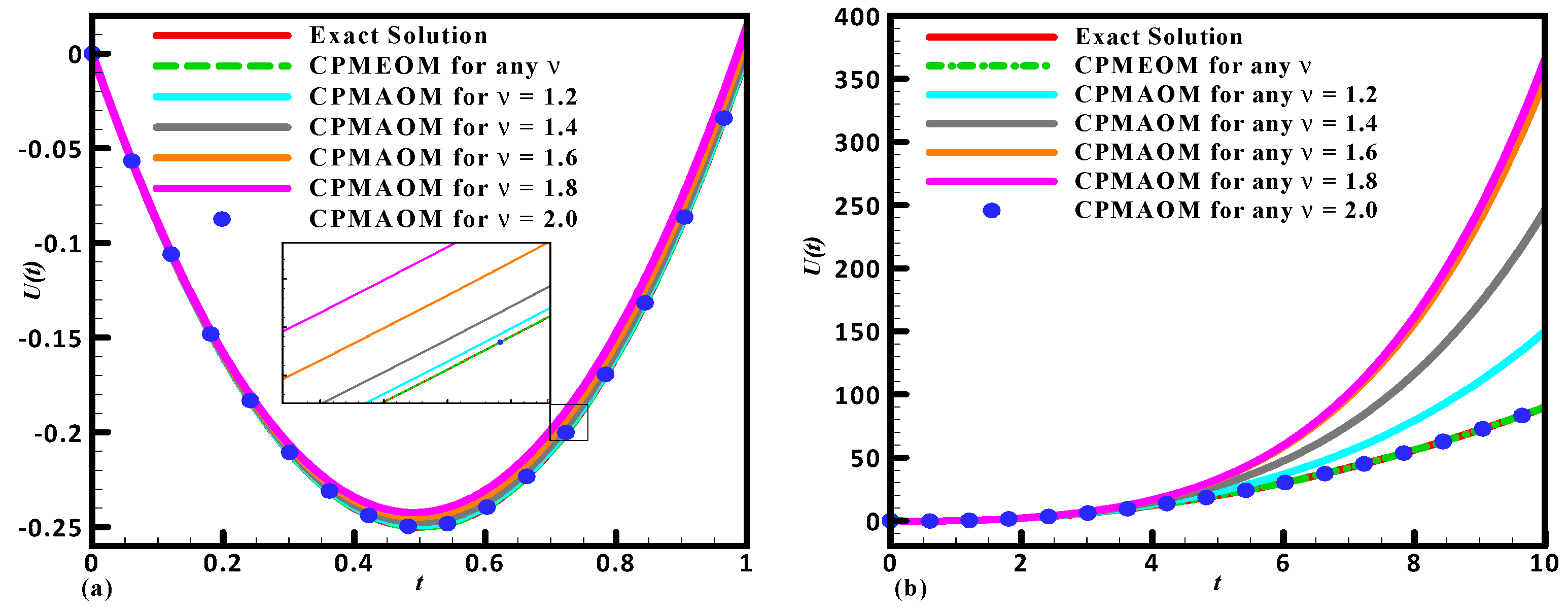
Figure 4.
The graphical representation of (Problem 1) exact solution, CPM solution via and CPM soliton via . The values of are chosen as (a) For and (b) For and .
Figure 4.
The graphical representation of (Problem 1) exact solution, CPM solution via and CPM soliton via . The values of are chosen as (a) For and (b) For and .
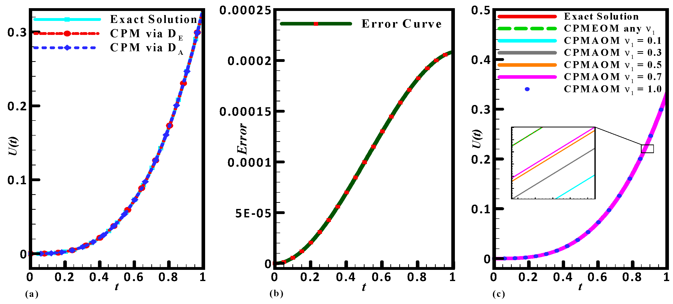
Figure 5.
The graphical representation of Problem 1 exact solution, CPM solution via and CPM soliton via (a) When are integer and (b) Error curve for CPMAOM. (c) Comparative study for different orders of derivatives.
Figure 5.
The graphical representation of Problem 1 exact solution, CPM solution via and CPM soliton via (a) When are integer and (b) Error curve for CPMAOM. (c) Comparative study for different orders of derivatives.
Figure 6.
The graphical representation of Bagley–Torvik (BT)-equation. (a) Exact solution, CPM solution via and CPM solution via . (b) Error curve for CPMAOM.
Figure 6.
The graphical representation of Bagley–Torvik (BT)-equation. (a) Exact solution, CPM solution via and CPM solution via . (b) Error curve for CPMAOM.
Table 1.
Comparative analysis between algorithms based on both kinds of operational matrices and when and various values of .
Table 1.
Comparative analysis between algorithms based on both kinds of operational matrices and when and various values of .
| t | | | | | | |
|---|
| |
| | | | | |
|---|
| 0.1 | 0 | 8.18856 × 10⁻³ | 4.92337 × 10⁻⁴ | 3.22352 × 10⁻⁴ | 2.05608 × 10⁻⁴ | 2.56707 × 10⁻⁴ |
| 0.2 | 0 | 2.86418 × 10⁻³ | 1.83398 × 10⁻³ | 1.19962 × 10⁻³ | 7.64621 × 10⁻⁴ | 9.54227 × 10⁻³ |
| 0.3 | 0 | 5.60085 × 10⁻³ | 3.82190 × 10⁻³ | 2.49712 × 10⁻³ | 1.59032 × 10⁻³ | 1.98366 × 10⁻³ |
| 0.4 | 0 | 8.60270 × 10⁻³ | 6.25305 × 10⁻³ | 4.08017 × 10⁻³ | 2.59599 × 10⁻³ | 3.23609 × 10⁻³ |
| 0.5 | 0 | 1.15525 × 10⁻² | 8.92438 × 10⁻³ | 5.81409 × 10⁻³ | 3.69492 × 10⁻³ | 4.60263 × 10⁻³ |
| 0.6 | 0 | 1.42422 × 10⁻² | 1.16328 × 10⁻³ | 7.56419 × 10⁻³ | 4.80038 × 10⁻³ | 5.97436 × 10⁻³ |
| 0.7 | 0 | 1.65723 × 10⁻² | 1.41754 × 10⁻² | 9.19580 × 10⁻³ | 5.82566 × 10⁻³ | 7.24239 × 10⁻³ |
| 0.8 | 0 | 1.85527 × 10⁻² | 1.63491 × 10⁻² | 1.05742 × 10⁻² | 6.68405 × 10⁻³ | 8.29782 × 10⁻³ |
| 0.9 | 0 | 2.03021 × 10⁻² | 1.79507 × 10⁻² | 1.15648 × 10⁻³ | 7.28881 × 10⁻³ | 9.03173 × 10⁻³ |
| 1.0 | 0 | 2.20482 × 10⁻² | 1.87773 × 10⁻² | 1.20328 × 10⁻² | 7.55325 × 10⁻³ | 9.33523 × 10⁻³ |
Table 2.
Comparative analysis of Problem 1 with exact solution and solutions obtained via Chelyshkov polynomial method (CPM) via and when .
Table 2.
Comparative analysis of Problem 1 with exact solution and solutions obtained via Chelyshkov polynomial method (CPM) via and when .
| [39] | [40] | | | |
|---|
| |
|---|
| 0.1 | 9.2677 × 10⁻⁷ | 1.4411 × 10⁻⁴ | 1.96538 × 10⁻⁴ | 0 | 0 | 0 |
| 0.2 | 3.6193 × 10⁻⁶ | 1.4007 × 10⁻⁴ | 7.30757 × 10⁻⁴ | 0 | 0 | 0 |
| 0.3 | 6.3739 × 10⁻⁶ | 1.3459 × 10⁻⁴ | 1.51957 × 10⁻³ | 0 | 0 | 0 |
| 0.4 | 9.1427 × 10⁻⁶ | 1.2835 × 10⁻⁴ | 2.47987 × 10⁻³ | 0 | 0 | 0 |
| 0.5 | 1.2129 × 10⁻⁵ | 1.2241 × 10⁻⁴ | 3.52859 × 10⁻³ | 0 | 0 | 0 |
| 0.6 | 1.4512 × 10⁻⁵ | 1.1491 × 10⁻⁴ | 4.58261 × 10⁻³ | 0 | 0 | 0 |
| 0.7 | 1.7072 × 10⁻⁵ | 1.0803 × 10⁻⁴ | 5.55886 × 10⁻³ | 0 | 0 | 0 |
| 0.8 | 1.9533 × 10⁻⁵ | 1.0114 × 10⁻⁴ | 6.37425 × 10⁻³ | 0 | 0 | 0 |
| 0.9 | 2.1888 × 10⁻⁵ | 9.4240 × 10⁻⁴ | 6.94567 × 10⁻³ | 0 | 0 | 0 |
Table 3.
Comparative analysis between algorithms based on both kinds of operational matrices and when and various values of .
Table 3.
Comparative analysis between algorithms based on both kinds of operational matrices and when and various values of .
| | | | | | |
|---|
| |
| | | | | |
|---|
| 0.1 | 0 | 6.88784 × 10⁻⁵ | 2.08680 × 10⁻⁴ | 5.70950 × 10⁻⁴ | 5.70950 × 10⁻⁴ | 0 |
| 0.2 | 0 | 2.25898 × 10⁻⁴ | 6.96022 × 10⁻⁴ | 1.98169 × 10⁻³ | 1.98169 × 10⁻³ | 0 |
| 0.3 | 0 | 4.09948 × 10⁻⁴ | 1.28895 × 10⁻³ | 3.84296 × 10⁻³ | 3.84296 × 10⁻³ | 0 |
| 0.4 | 0 | 5.77665 × 10⁻⁴ | 1.86103 × 10⁻³ | 5.85077 × 10⁻³ | 5.85076 × 10⁻³ | 0 |
| 0.5 | 0 | 7.03432 × 10⁻⁴ | 2.33245 × 10⁻³ | 7.78631 × 10⁻³ | 7.78631 × 10⁻³ | 0 |
| 0.6 | 0 | 7.79381 × 10⁻⁴ | 2.67003 × 10⁻³ | 9.51603 × 10⁻³ | 9.51603 × 10⁻³ | 0 |
| 0.7 | 0 | 8.15394 × 10⁻⁴ | 2.88722 × 10⁻³ | 1.09916 × 10⁻² | 1.09916 × 10⁻² | 0 |
| 0.8 | 0 | 8.39099 × 10⁻⁴ | 3.04411 × 10⁻³ | 1.22500 × 10⁻² | 1.22500 × 10⁻² | 0 |
| 0.9 | 0 | 8.95872 × 10⁻⁴ | 3.24741 × 10⁻³ | 1.34132 × 10⁻² | 1.34132 × 10⁻² | 0 |
| 1.0 | 0 | 1.04884 × 10⁻³ | 3.65048 × 10⁻³ | 1.46887 × 10⁻² | 1.46887 × 10⁻² | 0 |
Table 4.
Comparative analysis between algorithms based on both kinds of operational matrices and when and various values of .
Table 4.
Comparative analysis between algorithms based on both kinds of operational matrices and when and various values of .
| | | | | | |
|---|
| | | | | |
|---|
| 0.1 | 0 | 8.76067 × 10⁻⁶ | 5.87688 × 10⁻⁶ | 3.91584 × 10⁻⁶ | 3.62176 × 10⁻⁶ | 5.54734 × 10⁻⁶ |
| 0.2 | 0 | 3.26440 × 10⁻⁵ | 2.18920 × 10⁻⁵ | 1.45838 × 10⁻⁵ | 1.34754 × 10⁻⁵ | 2.06163 × 10⁻⁵ |
| 0.3 | 0 | 6.80521 × 10⁻⁵ | 4.56220 × 10⁻⁵ | 3.03845 × 10⁻⁵ | 2.80434 × 10⁻⁵ | 4.28474 × 10⁻⁵ |
| 0.4 | 0 | 1.11387 × 10⁻⁴ | 7.46435 × 10⁻⁵ | 4.96987 × 10⁻⁵ | 4.58084 × 10⁻⁵ | 6.98811 × 10⁻⁵ |
| 0.5 | 0 | 1.59050 × 10⁻⁴ | 1.06533 × 10⁻⁴ | 7.09070 × 10⁻⁵ | 6.52528 × 10⁻⁵ | 9.93578 × 10⁻⁵ |
| 0.6 | 0 | 2.07445 × 10⁻⁴ | 1.38868 × 10⁻⁴ | 9.23900 × 10⁻⁵ | 8.48591 × 10⁻⁵ | 1.28918 × 10⁻⁴ |
| 0.7 | 0 | 2.52972 × 10⁻⁴ | 1.69224 × 10⁻⁴ | 1.12528 × 10⁻⁴ | 1.03110 × 10⁻⁴ | 1.56202 × 10⁻⁴ |
| 0.8 | 0 | 2.92034 × 10⁻⁴ | 1.95179 × 10⁻⁴ | 1.29703 × 10⁻⁴ | 1.18488 × 10⁻⁴ | 1.78850 × 10⁻⁴ |
| 0.9 | 0 | 3.21033 × 10⁻⁴ | 2.14308 × 10⁻⁴ | 1.42294 × 10⁻⁴ | 1.29475 × 10⁻⁴ | 1.94504 × 10⁻⁴ |
| 1.0 | 0 | 3.36371 × 10⁻⁴ | 2.24189 × 10⁻⁴ | 1.48682 × 10⁻⁴ | 1.34554 × 10⁻⁴ | 2.00802 × 10⁻⁴ |
Table 5.
Comparative analysis of Problem 2 with exact solution, existing literature and solutions obtained via Chelyshkov polynomial method (CPM) via and when
Table 5.
Comparative analysis of Problem 2 with exact solution, existing literature and solutions obtained via Chelyshkov polynomial method (CPM) via and when
| [39] | [40] | | | |
|---|
| |
|---|
| 0.1 | 2.9095 × 10⁻⁷ | 5.8178 × 10⁻⁴ | 5.46485 × 10⁻⁶ | 0 | 0 | 0 |
| 0.2 | 7.5117 × 10⁻⁷ | 5.7770 × 10⁻⁴ | 2.03565 × 10⁻⁵ | 0 | 0 | 0 |
| 0.3 | 1.2248 × 10⁻⁷ | 5.5994 × 10⁻⁴ | 4.24208 × 10⁻⁵ | 0 | 0 | 0 |
| 0.4 | 4.8091 × 10⁻⁷ | 5.3877 × 10⁻⁴ | 6.94033 × 10⁻⁵ | 0 | 0 | 0 |
| 0.5 | 1.6932 × 10⁻⁷ | 5.1798 × 10⁻⁴ | 9.90498 × 10⁻⁵ | 0 | 0 | 0 |
| 0.6 | 2.1874 × 10⁻⁶ | 4.8878 × 10⁻⁴ | 1.29106 × 10⁻⁴ | 0 | 0 | 0 |
| 0.7 | 2.5735 × 10⁻⁶ | 4.6190 × 10⁻⁴ | 1.57318 × 10⁻⁴ | 0 | 0 | 0 |
| 0.8 | 2.9814 × 10⁻⁶ | 4.3484 × 10⁻⁴ | 1.81430 × 10⁻⁴ | 0 | 0 | 0 |
| 0.9 | 3.7412 × 10⁻⁶ | 1.0522 × 10⁻⁴ | 1.99190 × 10⁻⁴ | 0 | 0 | 0 |
Table 6.
Comparative analysis between algorithms based on both kinds of operational matrices and when and various values of .
Table 6.
Comparative analysis between algorithms based on both kinds of operational matrices and when and various values of .
| | | | | | |
|---|
| | | | | | | |
|---|
| 0.1 | 0 | 0 | 3.89289 × 10⁻⁶ | 1.33259 × 10⁻⁵ | 2.08402 × 10⁻⁵ | 1.94482 × 10⁻⁵ |
| 0.2 | 0 | 0 | 1.45018 × 10⁻⁵ | 4.97146 × 10⁻⁵ | 7.80106 × 10⁻⁵ | 7.31324 × 10⁻⁵ |
| 0.3 | 0 | 0 | 3.02220×10⁻⁵ | 1.03782 × 10⁻⁴ | 1.63485 × 10⁻⁴ | 1.54062 × 10⁻⁴ |
| 0.4 | 0 | 0 | 4.94490 × 10⁻⁵ | 1.70145 × 10⁻⁴ | 2.69239 × 10⁻⁴ | 2.55246 × 10⁻⁴ |
| 0.5 | 0 | 0 | 7.05780 × 10⁻⁵ | 2.43420 × 10⁻⁴ | 3.87247 × 10⁻⁴ | 3.69695 × 10⁻⁴ |
| 0.6 | 0 | 0 | 9.20044 × 10⁻⁵ | 3.18223 × 10⁻⁴ | 5.09482 × 10⁻⁴ | 4.90417 × 10⁻⁴ |
| 0.7 | 0 | 0 | 1.12124 × 10⁻⁴ | 3.89170 × 10⁻⁴ | 6.27919 × 10⁻⁴ | 6.10421 × 10⁻⁴ |
| 0.8 | 0 | 0 | 1.29331 × 10⁻⁴ | 4.50878 × 10⁻⁴ | 7.34533 × 10⁻⁴ | 7.22718 × 10⁻⁴ |
| 0.9 | 0 | 0 | 1.42022 × 10⁻⁴ | 4.97963 × 10⁻⁴ | 8.21298 × 10⁻⁴ | 8.20316 × 10⁻⁴ |
| 1.0 | 0 | 0 | 1.48591 × 10⁻⁴ | 5.25041 × 10⁻⁴ | 8.80189 × 10⁻⁴ | 8.96226 × 10⁻⁴ |
Table 7.
Comparative analysis between algorithms based on both kinds of operational matrices and when and various values of .
Table 7.
Comparative analysis between algorithms based on both kinds of operational matrices and when and various values of .
| | | |
|---|
| | | | | |
|---|
| 0.1 | 0 | 1.64747 × 10⁻³ | 0 | 1.62187 × 10⁻³ | 0 | 1.61491 × 10⁻³ |
| 0.2 | 0 | 6.58986 × 10⁻³ | 0 | 6.48749 × 10⁻³ | 0 | 6.45966 × 10⁻³ |
| 0.3 | 0 | 1.48272 × 10⁻² | 0 | 1.45969 × 10⁻² | 0 | 1.45342 × 10⁻² |
| 0.4 | 0 | 2.63595 × 10⁻² | 0 | 2.59500 × 10⁻² | 0 | 2.58386 × 10⁻² |
| 0.5 | 0 | 4.11867 × 10⁻² | 0 | 4.05468 × 10⁻² | 0 | 4.03729 × 10⁻² |
| 0.6 | 0 | 5.93088 × 10⁻² | 0 | 5.83874 × 10⁻² | 0 | 5.81369 × 10⁻² |
| 0.7 | 0 | 8.07258 × 10⁻² | 0 | 7.94718 × 10⁻² | 0 | 7.91308 × 10⁻² |
| 0.8 | 0 | 1.05438 × 10⁻¹ | 0 | 1.03800 × 10⁻¹ | 0 | 1.03355 × 10⁻¹ |
| 0.9 | 0 | 1.33445 × 10⁻¹ | 0 | 1.31372 × 10⁻¹ | 0 | 1.30808 × 10⁻¹ |
| 1.0 | 0 | 1.64747 × 10⁻¹ | 0 | 1.62187 × 10⁻¹ | 0 | 1.61491 × 10⁻¹ |
Table 8.
L2 error analysis for various values of time and comparison between both kinds of methods.
Table 8.
L2 error analysis for various values of time and comparison between both kinds of methods.
| | | | |
|---|
| CPMEOM | CPMAOM | CPMEOM | CPMAOM | CPMEOM | CPMAOM | CPMEOM | CPMAOM |
|---|
| 0.2 | 0 | 7.553 × 10⁻⁶ | 0 | 7.165 × 10⁻⁸ | 0 | 2.852 × 10⁻⁹ | 0 | 7.126 × 10⁻¹⁰ |
| 0.4 | 0 | 3.193 × 10⁻⁵ | 0 | 2.883 × 10⁻⁷ | 0 | 1.142 × 10⁻⁸ | 0 | 2.852 × 10⁻⁹ |
| 0.6 | 0 | 7.572 × 10⁻⁵ | 0 | 6.526 × 10⁻⁷ | 0 | 2.573 × 10⁻⁸ | 0 | 6.422 × 10⁻⁹ |
| 0.8 | 0 | 1.415 × 10⁻⁴ | 0 | 1.167 × 10⁻⁶ | 0 | 4.580 × 10⁻⁸ | 0 | 1.142 × 10⁻⁸ |
| 1.0 | 0 | 2.319 × 10⁻⁴ | 0 | 1.834 × 10⁻⁶ | 0 | 7.165 × 10⁻⁸ | 0 | 1.786 × 10⁻⁸ |
Table 9.
L∞ error analysis for various values of time and comparison between both kinds of methods.
Table 9.
L∞ error analysis for various values of time and comparison between both kinds of methods.
| | | | |
|---|
| CPMEOM | CPMAOM | CPMEOM | CPMAOM | CPMEOM | CPMAOM | CPMEOM | CPMAOM |
|---|
| 0.2 | 0 | 2.696 × 10⁻⁶ | 0 | 2.227 × 10⁻⁸ | 0 | 8.742 × 10⁻¹⁰ | 0 | 2.180 × 10⁻¹⁰ |
| 0.4 | 0 | 1.287 × 10⁻⁵ | 0 | 9.118 × 10⁻⁸ | 0 | 3.514 × 10⁻⁹ | 0 | 8.742 × 10⁻¹⁰ |
| 0.6 | 0 | 3.362 × 10⁻⁵ | 0 | 2.098 × 10⁻⁷ | 0 | 7.943 × 10⁻⁹ | 0 | 1.972 × 10⁻⁹ |
| 0.8 | 0 | 6.806 × 10⁻⁵ | 0 | 3.814 × 10⁻⁷ | 0 | 1.419 × 10⁻⁸ | 0 | 3.514 × 10⁻⁹ |
| 1.0 | 0 | 1.193 × 10⁻⁴ | 0 | 6.090 × 10⁻⁷ | 0 | 2.227 × 10⁻⁸ | 0 | 5.503 × 10⁻⁹ |
Table 10.
Root mean square (RMS) error analysis for various values of time and comparison between both kinds of methods.
Table 10.
Root mean square (RMS) error analysis for various values of time and comparison between both kinds of methods.
| | | | |
|---|
| CPMEOM | CPMAOM | CPMEOM | CPMAOM | CPMEOM | CPMAOM | CPMEOM | CPMAOM |
|---|
| 0.2 | 0 | 2.388 × 10⁻⁶ | 0 | 7.165 × 10⁻⁹ | 0 | 1.276 × 10⁻¹⁰ | 0 | 2.254 × 10⁻¹¹ |
| 0.4 | 0 | 1.010 × 10⁻⁵ | 0 | 2.883 × 10⁻⁸ | 0 | 5.109 × 10⁻¹⁰ | 0 | 9.020 × 10⁻¹¹ |
| 0.6 | 0 | 2.395 × 10⁻⁵ | 0 | 6.526 × 10⁻⁸ | 0 | 1.151 × 10⁻⁹ | 0 | 2.031 × 10⁻¹⁰ |
| 0.8 | 0 | 4.475 × 10⁻⁵ | 0 | 1.167 × 10⁻⁷ | 0 | 2.048 × 10⁻⁹ | 0 | 3.612 × 10⁻¹⁰ |
| 1.0 | 0 | 7.332 × 10⁻⁵ | 0 | 1.834 × 10⁻⁷ | 0 | 3.204 × 10⁻⁹ | 0 | 5.648 × 10⁻¹⁰ |
