Article

GRID: GRID Resample by Information Distribution

1
Institute of Intelligent Control and Image Engineering, Xidian University, Xi’an 710071, China
2
China Academy of Space Technology, Haidian 100094, Beijing, China
*
Author to whom correspondence should be addressed.
Symmetry 2020, 12(9), 1417; https://doi.org/10.3390/sym12091417
Submission received: 20 July 2020 / Revised: 17 August 2020 / Accepted: 22 August 2020 / Published: 26 August 2020
(This article belongs to the Section Computer)

Abstract

:
This paper exploits a concise yet efficient initialization strategy to optimize grid sampling-based superpixel segmentation algorithms. Rather than straight distributing all initial seeds evenly, it adopts a context-aware approach to modify their positions and total number via a coarse-to-fine manner. Firstly, half the expected number of seeds are regularly sampled on the image grid, thereby creating a rough distribution of color information for all rectangular cells. A series of fission is then performed on cells that contain excessive color information recursively. In each cell, the local color uniformity is balanced by a dichotomy on one original seed, which generates two new seeds and settles them to spatially symmetrical sub-regions. Therefore, the local concentration of seeds is adaptive to the complexity of regional information. In addition, by calculating the amount of color via a summed area table (SAT), the informative regions can be located at a very low time cost. As a result, superpixels are produced from ideal original seeds with an exact number and exhibit better boundary adherence. Experiments demonstrate that the proposed strategy effectively promotes the performance of simple linear iterative clustering (SLIC) and its variants in terms of several quality measures.

1. Introduction

Superpixels are commonly regarded as the results of grouping perceptually meaningful connected regions of an image. Since the concept is introduced in [1], an increasing number of superpixel algorithms are put forward to replace the pixel-level features to help speed up other tasks. Over the last few years, superpixels have gradually become fundamental and significant in the field of image processing and computer vision domains. Many advanced visual applications, such as image stitching [2], target tracking [3], video object segmentation [4], saliency detection [5] and depth estimation [6], have been developed based on superpixel segmentation. It serves as an effective method for computing image features and greatly reduces the number of entities. It therefore remains a hotspot in the research from its birth to the present.
Existing superpixel methods can be divided into various categories according to different classification criteria. Stutz et al. [7] roundly reviewed the mainstream and divided them into eight categories, which is considered to be one of the most comprehensive surveys. Considering the segmentation model, in this paper, they are roughly classified as graph-based and gradient-based methods. In general, these two classes of methods provide an eligibly balanced trade-off for the task at hand, which are expected to be more appropriate for deployment and expansion. Therefore, some representative methods of these two categories are mainly reviewed below. In addition, a brief review of seed-demand superpixels is presented at the end of this section.

1.1. Graph-Based Superpixel Segmentation

A graph-based method builds a node adjacency graph to represent an image. In the graph model, each pixel is regarded as a node, and the edge connecting two nodes represents the similarity between the two pixels. The superpixel generation task is then converted into minimizing the costs of cut defined on the graph. Known for the foundation of superpixels, Normalized Cuts (NC) [8] is a typical algorithm that uses contour and texture information to construct the graph and then globally minimizes a cost function defined on the edges at the partition boundaries. Among the early superpixel algorithms, NC is the only one that implicitly considers spatial compactness. However, as a NP-hard problem, it shows highly time-consuming, which limits its applicability. Random Walks (RW) [9] is another typical graph-based approach as well as an interactive image segmentation. The seeds of foreground and background objects are manually specified by the user. Based on the probability of each unlabeled node arriving at each seed pixel for the first time, the unlabeled nodes are divided and the final segmentation result is obtained.
To further improve these algorithms, some combinational optimizations are adopted to reduce the computational complexity or elevate superpixel compactness and boundary adherence. In Entropy Rate Superpixel (ERS) [10], an objective function based on the entropy rate of a random walk on the graph modeled by the image is proposed. Since the energy function consists of color and boundary terms, it results in encouraging superpixels with homogeneous color and regular size. Lazy Random Walk (LRW) [11] superpixel segmentation integrates the compactness constraint into lazy random walks by considering the global relationships between all the pixels and the seed points, which can produce compact superpixels with desirable performance in weak boundary and complex texture regions. Dynamic Random Walk (DRW) [12] adds a new type of dynamic node to the conventional RW model, which reduces redundant calculation by limiting the walking range. The energy function of the RW is redefined in order to address the problem of seed-lacking. In addition, it adopts the first arrival probability between each pair of nodes to avoid the interference for each partition. As a result, DRW superpixels increase the boundary adherence with linear time complexity.

1.2. Gradient-Based Superpixel Segmentation

Gradient-based methods propose the idea of clustering the pixels along the directions that the gradients change most quickly. As a consequence, the classified pixels are grouped into different superpixels. Simple Linear Iterative Clustering (SLIC) [13] firstly adopts the concept of restricting search ranges to the superpixel segmentation. It runs local k-means clustering with a weighted distance measure combining color and spatial proximity, resulting in controllability over the size and compactness of the superpixels, and significant efficiency improvement. Based on the topological theory with mathematical morphology, watershed [14] is another form of gradient ascent approach. It treats the gradient image as a topographic surface and then floods from the minima based on region-growing. As a result, the image can be partitioned into catchment basins and watershed lines, corresponding to the homogeneous superpixel regions.
Owing to these enlightening approaches, various efforts are put forward to improve the performance. Superpixels with Contour Adherence using Linear Path (SCALP) [15] introduces a novel robust distance to boost the properties. Considering the color features along the linear path between the pixel and the corresponding superpixel barycenter, it can produce accurate, regular and robust superpixels. Intrinsic Manifold SLIC (IMSLIC) [16] extends SLIC by an elaborate distance measurement and a two-dimensional manifold feature space mapping. The new framework can make superpixels sensitive to image content, thus producing better boundary adherence. Fast Linear Iterative Clustering (FLIC) [17] presents a novel active search strategy by relationships between neighboring pixels, which takes the place of fixed search ranges in other variants of SLIC and achieves rapid convergence of linear clustering.
Besides the iteration-needed methods, in recent years, superpixel generation in a one-pass fashion has gained more attention. Owing to the non-iterative implementation, it fundamentally reduces the computational cost of optimization procedures. Achanta et al. [18] proposed Simple Non-Iterative Clustering (SNIC) to promote the computing efficiency of SLIC, which adopts a priority queue and a joint assignment and update framework to generate superpixels without iteration. In [19], an adaptive sampling strategy is taken to assign superpixels to image regions reconstructed by spatial and color quantization, then pixels and superpixels are reassigned by maximum a posteriori by spatial and visual similarities as well as refinement. In order to influence the compactness of watershed algorithms that over-segment an image without iteration, Watershed Superpixels (WS) [20] and Compact Watershed (CW) [21] introduce spatial constraint to a SLIC-like grid, respectively. Both of these two changes could produce uniform watershed superpixels with controllability of the number and regularity. In Waterpixels [22], a family of methods based on the watershed transformation is introduced to compute superpixels. The proposed Waterpixels show desirable quality and speed, which offers an interesting perspective for superpixel approaches.

1.3. Background of Seed-Demand Superpixels

Among all of the abovementioned algorithms, [11,12,13,14,15,16,17,18,19,20,21,22] is seed-demand, except for [14]. They all produce superpixels by initializing a set of evenly distributed seeds on a regular grid, and then grow superpixels from the corresponding pixels. Nevertheless, it is merely proposed to produce approximately the same size superpixels with the expected number, without concerning any varying content of the input image. In other words, this strategy is essentially a data-driven implementation following a bottom-up manner. Thus, the algorithms utilize only color and spatial features, which result in inferior segmentation performance when the color feature is inadequate [23]. For example, the real-world images usually contain highly variable features, leading to textured regions together with homogeneous ones. Although the positions of the seeds can be updated by regional iterations, the probability of covering small objects is still weak.
Since the core of seed-demand superpixel algorithms is to determine the final locations of all cluster centers efficiently, a good initialization step for seeds is necessary to achieve good segmentation performance. Particle-Filter-based Superpixel (PFS) [24] converts the superpixel generation into a multiple-region particle filter problem. It assigns several initial particles to each block based on the density function and association rule. This strategy is beneficial for the propagation step, and the cluster centers avoid falling into local optimum that generate more homogenous superpixels. However, like many other algorithms, PFS fails to produce exactly the same number of superpixels required by the user due to the grid sampling. In IMSLIC, a new seed initialization approach is proposed, which randomly generates seeds on a two-dimensional manifold whose area elements are a good measure of content density. The seeds are densely distributed in content-dense regions and sparsely distributed in other regions after projecting them back to the image plane. By averaging the distribution of areas in both the image plane and curved manifold, DRW produces seeds that cover the objects as much as possible. Therefore, the seeds are very well distributed to cover the small objects or strip areas. Unlike gradient-based methods, the positions of all seeds of DRW are stationary throughout the superpixel-generating process. Whereas it can improve the boundary adherence of resulting superpixels, the initialization strategy is only suitable for RW-like methods.
This paper mainly focuses on further promoting the performance of gradient-based superpixel algorithms by optimizing the initialization step. A new strategy referred to as GRID Resample by Information Distribution (GRID) is being applied for seed-demand approaches. It incorporates two stages of seeding with a coarse-to-fine manner via an information-theoretic perspective. In the first stage, a regular grid of the input image is formed by evenly distributing half the expected number of seeds in all rectangular cells with a larger size. It is done to roughly estimate the amount of information stored in each cell. As indicated by the recursive acronym, in the second stage, the proposed GRID performs recursive fission operations on seeds whose grid cells contain more color components. By splitting one seed into two and then settling them to different sub-regions, the content of color information in the original cell region is moderated. Finally, the local concentration of seeds adapts the complexity of regional information. As a result, complicated texture and small size regions are easy to be assigned more seeds, while a wide range of homogenous backgrounds also acquires sufficient seeds for segmentation.
It is worth noting that the amount of color information is calculated by a Summed Area Table (SAT) in the first stage. Therefore, the local content can be quickly obtained during the recursion in the second stage. In addition, the order of seed dichotomy is sorted by a priority queue, which could terminate the recursive fission operation once the exact number specified by the user is achieved. Compared with the conventional grid sampling initialization, the proposed GRID appreciably improves the performance and can be easily embedded into the main framework of superpixel algorithms. Experimental results on the public dataset verify the effectiveness via several quantitative metrics, which provide a desirable trade-off between time efficiency and segmentation accuracy.
This paper is organized as follows. Four gradient-based methods superpixel algorithms are reviewed in the next section, with an emphasis on SLIC. In Section 3, an analysis of the grid sampling-based initialization method is given before comparing it with the proposed GRID. Qualitative and quantitative analyses are explicated in Section 4. Finally, Section 5 makes a brief conclusion.

2. Grid Sampling-Based Superpixel Segmentation

The proposed superpixel initialization method is mainly worked on grid sampling-based algorithms. Therefore, the conventional SLIC [13] and its three variants are chosen as baselines for further improvement. Within this section, a retrospection on the four algorithms are introduced in brief. Meanwhile, some key notations used in this paper are declared and explained in Table 1.

2.1. Simple Linear Iterative Clustering

SLIC is an iterative algorithm based on local k-means clustering, which improves the efficiency of Lloyd’s algorithm [25] and simplifies the calculation to get the Centroidal Voronoi Tessellation (CVT) [26]. The four-step process, including initialization, assignment, updating and merging, can be demonstrated as follows.
  • For a CIELAB color image I = { I i } i = 1 N with N pixels, its i th element I i can be described as a 5-dimensional feature vector F ( I i ) = [ l ( I i ) , a ( I i ) , b ( I i ) , x ( I i ) , y ( I i ) ] . Specifically, it is fused by a Lab color feature C ( I i ) = [ l ( I i ) , a ( I i ) , b ( I i ) ] and a coordinate of 2-dimensional Euclidean space P ( I i ) = [ x ( I i ) , y ( I i ) ] ;
  • A set of evenly distributed seeds { s k } k = 1 K are sampled on the image plane I , where K is a user-specified parameter to expect the number of superpixels. Thus, I is initially partitioned to a series of regular cells on the image gird with an interval of S = N / K .
  • In the assignment step, each pixel I i is assigned a label in accordance with the nearest cluster center s k based on a normalized Euclidean distance D ( I i , s k ) measured by
    D ( I i , s k ) = C ( I i ) C ( s k ) 2 2 + λ 2 P ( I i ) P ( s k ) 2 2 ,
    where λ is the quotient of maximal C ( I i ) and P ( I i ) within this cluster to normalize color and spatial proximity, and   2 represents the Euclidean metric;
  • During the updating step, a local k-means approach is adopted in a 2 S × 2 S search region based on D ( I i , s k ) . This is done to re-compute the cluster center with the feature vector
    F ( C ( s k ¯ ) , P ( s k ¯ ) ) = i Ω k [ C ( I i ) , P ( I i ) ] / | Ω k | ,
    where Ω k represents the cluster centered at P ( s k ¯ ) , | Ω k | is the number of pixels in Ω k . This procedure is performed on all K cluster regions and { s k } k = 1 K are then adjusted to { s k ¯ } k = 1 K . As a result, all pixels are associated with new labels, and the new centers of all search regions in the next loop are obtained. This step is iterated until it reaches a predefined global termination;
  • All disjoint components are merged to their neighboring superpixels by a region growing method, so that the connectivity among superpixels can be enforced heuristically.

2.2. SLIC-like Superpixel Segmentation

Thanks to the concise and enlightening framework, SLIC becomes specifically tailored to the problem of superpixel clustering. The following properties of SLIC are considered to be instructive:
  • It adopts a grid sampling strategy to distribute the incipient seeds during the initialization step. Therefore, the joint color–spatial space distance measurement in Equation (1) could both control the size and compactness of superpixels;
  • It firstly avoids performing redundant distance calculations by localizing the 2 S × 2 S search region in the assignment step, which reduces the time complexity of k-means from O ( k N ) to O ( N ) ;
  • It yields desirable adherence to image boundaries, and is faster and more memory efficient than existing methods.
This paper elaborately selects two follow-up works that are put forward to help SLIC become more outstanding from different aspects. They are FLIC [17] and SNIC [18], which effectively overcome the underlying limitation caused by the simplicity of SLIC, respectively.
A major insight of FLIC can be generalized as a trade-off between shape uniformity and time efficiency. It assumes that neighboring pixels have a natural continuity that tends to be assigned the same label. Basically, in the assignment step of conventional SLIC, only the distance metric D ( I i , s k ) in Equation (1) is adopted to iteratively classify the pixel I i . Differently, FLIC exploits the adjacent relationship of I i and its four neighboring elements { I j } j = 1 4 . Therefore, an active search method is proposed to make I i assign itself by
L ( I i ) = arg min L ( I j ) D ( I i , s L ( I j ) ) ,   i [ 1 , N ] ,   I j { I i } { I j } j = 1 4 .
where L (   ) means the final assigned label, s L ( I j ) is the cluster center of I j .
Based on the adjacent prior information, FLIC avoids the clusters being confined in fixed range in space, thus achieving more desirable boundary adherence. In addition, combined with the back-and-forth scan to traverse each superpixel, the active search method can be performed more efficiently. Moreover, the assignment and updating step work jointly, creating a synergistic effect that dramatically reduces the number of iterations.
SNIC works in a non-iterative manner that thoroughly avoids the iteration; it adopts a priority queue to achieve joint assignment and updating. The elaborate data structure continually records the newly explored elements inspected by all ever-expanding clusters. After an efficient heap sorting operation, it immediately returns an element I m with the minimum distance to a cluster center s k
I m = arg min D ( I i , s k ) , i [ 1 , N ] ,   k [ 1 , K ] .
Meanwhile, I m is assigned the label k by s k , and becomes a member of the cluster. In this way, a series of online averaging operations is performed on all clusters until the priority queue is empty.
Compared with SLIC, the non-iterative framework inspects each pixel 4 times at most [27], effectively preventing repeat computations in overlapping local regions. In practice, SNIC exhibits an identical O ( N ) complexity to SLIC. Moreover, this cluster expanding process maintains the spatial connectivity of pixels with the same labels. Therefore, the split-and-merge post-processing is omitted.
Another common SLIC-based variation is that the watershed segmentation adopts a SLIC-like initialization to boost the effect on the distribution of superpixels as well as on shape and size. WS [20] and CW [21] are two modified watershed segmentations [14] that could create uniformly shaped superpixels. Both of them incorporate a controllable compactness constraint in the marker-controlled watershed segmentation [28], which firstly adopts a subtle seeds extraction strategy to moderate conventional watershed segmentation. To make the superpixels more uniformly distributed than [28], WS and CW start with placing seeds in the image plane with an interval of S = N / K that is similar to SLIC. Besides, to force the compactness of the segmentation, they introduce a new metric to re-define the pixel priority in watershed
p ( I i ) = p g ( I i ) + λ p s ( I i ) ,
where p g ( I i ) is the priority of pixel I i in a gradient image, p s ( I i ) represents the priority that is quantized by the spatial constraint. λ is a normalized factor that balances two measurements, similar to Equation (1).
As mentioned above, the resulting priority metric is the weighted combination of conventional gradient magnitude value and the Euclidean distance of the pixel to the segment seed. A more precise spatial restriction is used in WS, which both takes edge information and pixel–seed distance into consideration. In addition, the watershed runs in O ( N log N ) that can be carried out with high efficiency empirically. The extra computation on compactness constraint only induces a slight increase in the practical runtime.

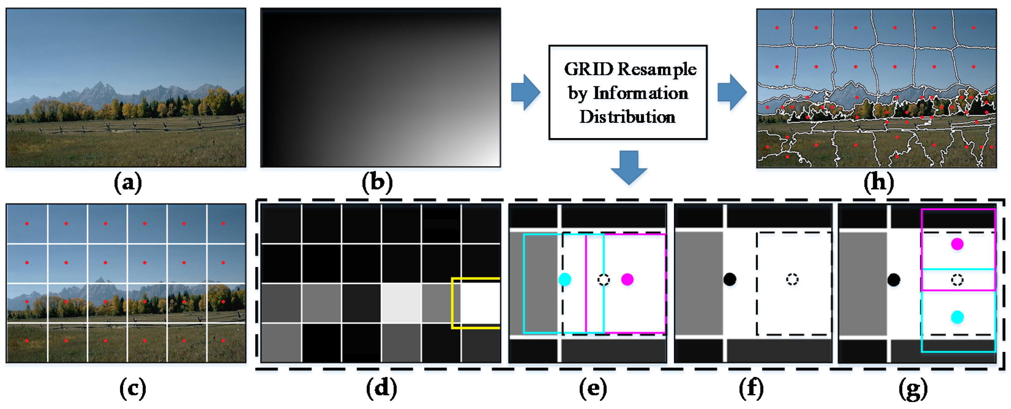
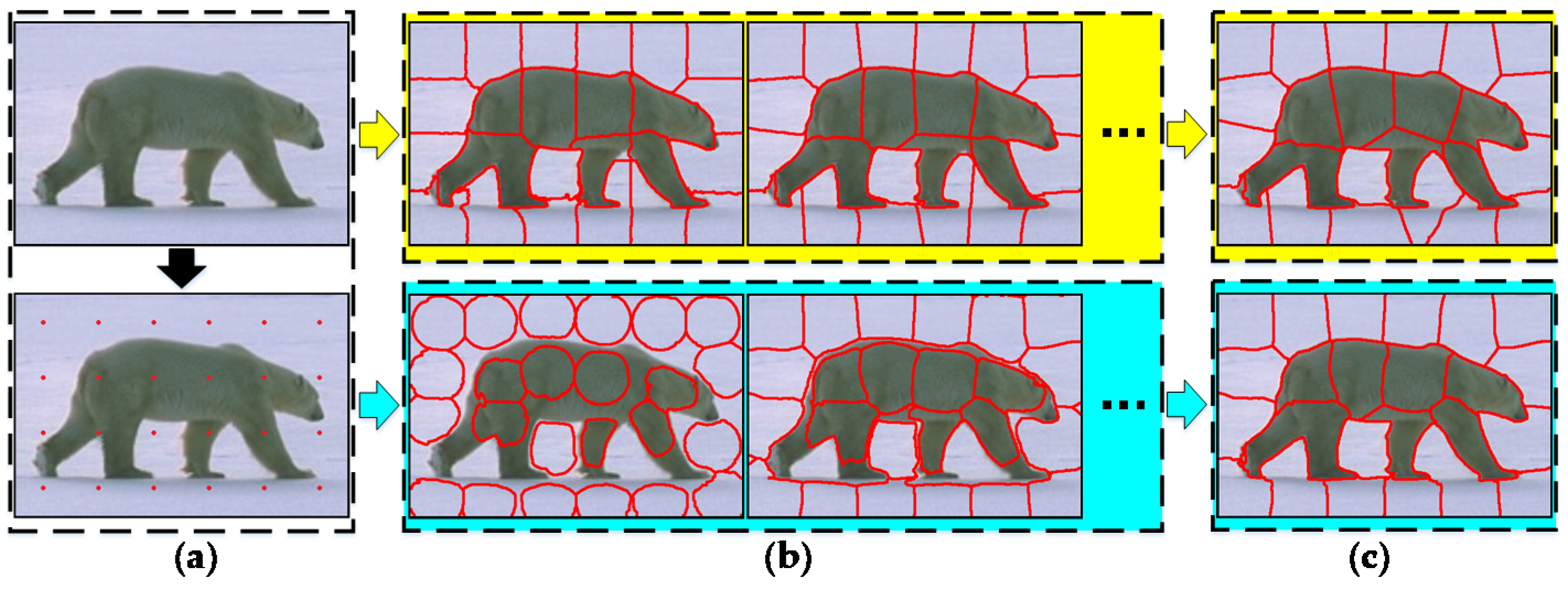
3. Proposed GRID Superpixel Initialization

This section introduces the proposed GRID strategy in detail. Firstly, an information-theoretic perspective is put forward to build an informative relationship of color homogeneity and grid sample for initial seeds. There is, however, a downside to the traditional grid-based distribution of seeds, which results in a bias of expected superpixel number. Based on the analysis above, a series of recursive sub-divisions on initial cells are performed using an adaptive resampling which sequentially splits an initial seed into two, thus achieving content-aware distribution of seeds. The schematic diagram of superpixel segmentation based on GRID initialization is illustrated in Figure 1.

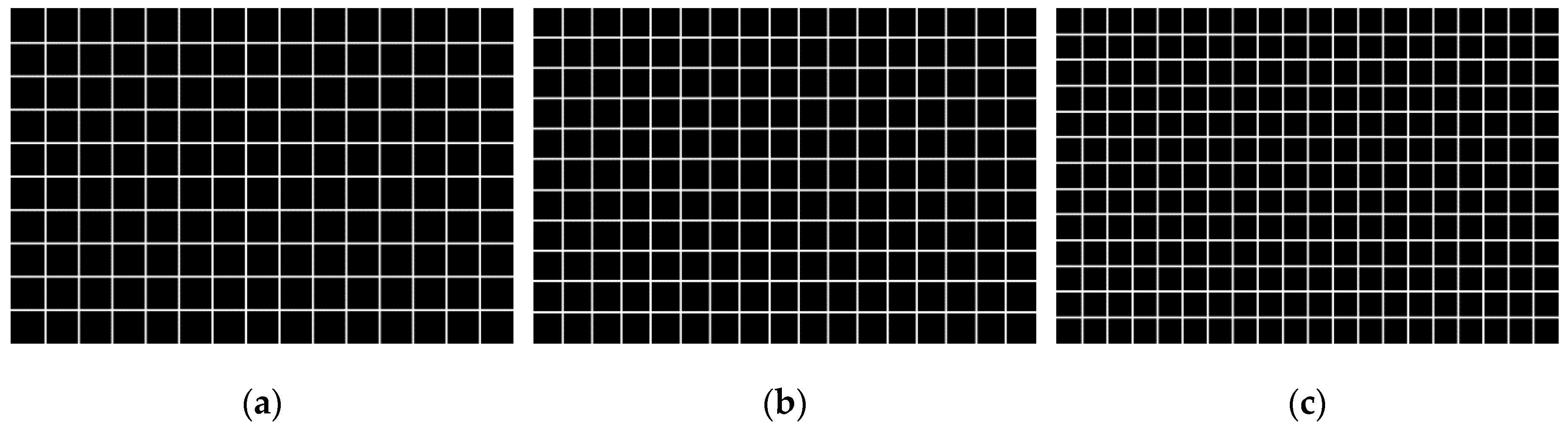
3.1. Analysis of Grid Sampling-Based Initialization

As demonstrated in the previous section, the core concept of gradient-based methods is clustering followed by continuously updating until all clusters converge. During the assignment and updating period, whether or not it performs self-renewal by iteration, each cluster seeks local homogeneity of color appearance. In other words, a superpixel is the result of minimizing the color content in a restricted region. In Figure 2, SLIC and FLIC iteratively classify the pixels in a 2 S × 2 S search region for each cluster center according to the color–spatial distance. Compared with the frequently re-labelled local pixels, SNIC and CW greedily generate superpixel regions by inspecting 4-neighbor elements and absorbing the most similar one repeatedly.
With the increasing number of initial seeds, the color content of each superpixel resembles a Gaussian distribution. As analyzed in [29], it can be modeled with a multivariate double exponential distribution as follows:
f ( C ; μ , σ ) = 1 Z exp ( ( C μ ) T ( C μ ) σ 2 ) ,
where Z is a normalization factor and σ is set to 1 for simplicity. Therefore, the total information contained in a superpixel can be calculated by
T ( Ω k ) = log i Ω k f ( C ( I i ) ; μ = C ( s k ¯ ) , σ = 1 ) = i Ω k C ( I i ) C ( s k ) 2 + constant
where C ( s k ¯ ) is the mean color of the cluster Ω k in Equation (1). It indicates that the amount of information of a superpixel equals the sum of color distances of all the pixels of the cluster to its average color and a constant. This formulation also reveals that the key to homogeneous superpixels is minimizing the color diversity in all clusters. Thus, for seed-demand superpixel algorithms, a good initialization means a lower expectation on the amount of color information for each resulting superpixel, or so-called lower content.
On the other side of the abovementioned methods, the initial seeds are sampled on regular grids as incipient cluster centers, which divide the input image I into several rectangular cells with the step of S = N / K . Let W and H denote the width and the height of I , respectively. In practice, the width w and height h of each rectangular region are given as follows [19]:
w = W S ,   h = H S .
Nevertheless, SLIC and its variants pursue an expected region with estimated size S × S for each superpixel, which requires an identity of w and h in Equation (8). To alleviate the contradiction caused by a different value of W and H , some boundary cells may adjust their own side length to maintain the main part as multiples of S × S . As shown in Figure 3, this may go against the number of superpixels specified by the user.
In practice, regional expansion approaches such as SNIC and Watershed seldom change the number of cells in the grid. Even if some seeds are located on edges or noise, these orphaned points can be avoided by perturbing in a 3 × 3 neighborhood to the lowest gradient position. Nonetheless, SLIC and FLIC, on the other hand, produce a large number of unconnected components since the connectivity in the joint spatial–color Euclidean space is not considered in Equation (1). Although they further apply some merging strategies, the number of resulting superpixels is still uncertain [16]. What is worse is that split-and-merge post-processing would produce heterogeneous regions, resulting in a bottleneck of performance.

3.2. Coarse-to-fine Seeds Modification by GRID

The goal of GRID is to produce a set of seeds that are context-aware to the local color and scale of an image. Seed-demand algorithms could then achieve good performance in generating superpixels with a precise number. This requirement can be translated into obtaining image segments in areas of low visual complexity with a larger number of homogeneous pixels, and high complexity with fewer heterogeneous pixels. As a result, a coarse-to-fine strategy that recursively modifies seeds positions and the total number is adopted in GRID. The major insight, as well as detailed steps, are demonstrated as follows:
  • The conventional grid sampling initialization with half the expected number of seeds is performed on the image plane. A set of evenly distributed seeds { s k } k = 1 K / 2 are sampled as the initial center of clusters.
  • The accumulation of lightness difference of all pixels in a S × S region from the center s k is calculated for simply representing the amount of color information in k th cell k
    A ( k ) = m k D l ( I m , s k ) = m k l ( I m ) l ( s k ) 2 .
    Compared with color dimensions a and b, the lightness L changes strongly in CIELAB color space, which also plays a major role in the color distance in Equation (1). Therefore, it is more efficient than accumulating the 3-channel color difference C ( I m ) C ( s k ) 2 in Equation (7).
  • A priority queue Q with decreasing order is introduced to hold all A ( k ) , which always returns the maximum element Q max that contains the greatest color information while it is not empty. These three steps are done to roughly establish an ordered distribution of color information for all rectangular cells on a larger scale.
  • Followed by recursive modifications on the positions and number of { s k } k = 1 K / 2 at a more precise level, Q max is acquired by popping the top-most element from Q , and the corresponding seed s m is divided into two new seeds s m 1 and s m 2 to balance the color information. Specifically, two new sub-regions m 1 and m 2 are delimited in m with 2/3 the area centered at s m 1 and s m 2 , respectively, which are also symmetric in the center of s m . The positions of the two new seeds are collinear with the original seed that minimizes the sum of A ( m 1 ) and A ( m 2 ) .
  • The new two seeds are pushed on Q for balancing the region containing global maximum information in the next loop. These last two steps are repeated till k increases to the exact number specified by the user.
It is worth noting that the Equation (4) can be recast into
A ( k ) = m k l ( I m ) l ( s k ) 2 = | m k l ( I m ) l ( s k ) × a r e a ( k ) | ,
where the first term m k l ( I m ) can be efficiently calculated by a summed area table (SAT). As known as the integral image, the SAT is first introduced to accelerate the computation of the Haar feature in [30]. It reduces the complexity of regional feature values O ( N ) to constant complexity O ( 4 ) . Before establishing the rough distribution of color information, the regional accumulation of lightness is calculated by a SAT
S A T ( x , y ) = x i < x , y i < y l ( x , y ) .
In the subsequent operations, computations on prior information of color distribution A ( m ) can be executed at a very low time cost by simple table lookups for SAT value in four vertices of m . The pseudo-code for the algorithm is presented in Algorithm 1.
Algorithm 1: GRID resample by information distribution framework
Input: the Lab image I , the expected superpixel number K
Output: the seeds set { s k } k = 1 K that number of elements is identical to K
/* Coarse Initialization */
calculate the summed area table of lightness in I .
initialize the seeds set { s k } k = 1 K / 2 similar to the conventional grid sampling method.
initialize a priority queue Q with decreasing order.
for each seed s k do
 calculate the amount of lightness information A ( k ) of the corresponding cell by Equation (9).
 create a vector node [ F ( s k ) , k , A ( k ) ] .
 push the node on Q .
end for
/* Recursive Modifications */
while the length of Q is not equal to K do
 pop the top-most node [ F ( s m ) , m , A ( m ) ] corresponding to s m from Q .
 divide s m into two new seeds s m 1 and s m 2 that contain the minimal A ( m 1 ) + A ( m 2 ) .
 create two vector nodes [ F ( s m 1 ) , m 1 , A ( m 1 ) ] and [ F ( s m 2 ) , m 2 , A ( m 2 ) ] , then push on Q .
end while
return the seeds set { s k } k = 1 K

4. Experiment and Analysis

The performance of the proposed GRID is evaluated on the Berkeley Segmentation Data Set 500 (BSDS500) [31], which comprises three image sets, training (100), validation (200) and testing (200). The images for segmentation are all 481 × 321 or 321 × 481 in size, along with manual ground truth. Superpixels produced by SLIC [13], FLIC [17], SNIC [18] and CW [21] are utilized as the reference group. The corresponding GRID-embedded algorithms termed as G-SLIC, G-FLIC, G-SNIC and G-CW are implemented as an experimental group to show their superiority, respectively. The default parameters of the available online code are used for a fair comparison, while only the round operation of the grid interval is modified on the basis of Equation (1). In addition, the gray value is used instead of lightness in CW and G-CW since they are performed on RGB color space rather than CIELAB.

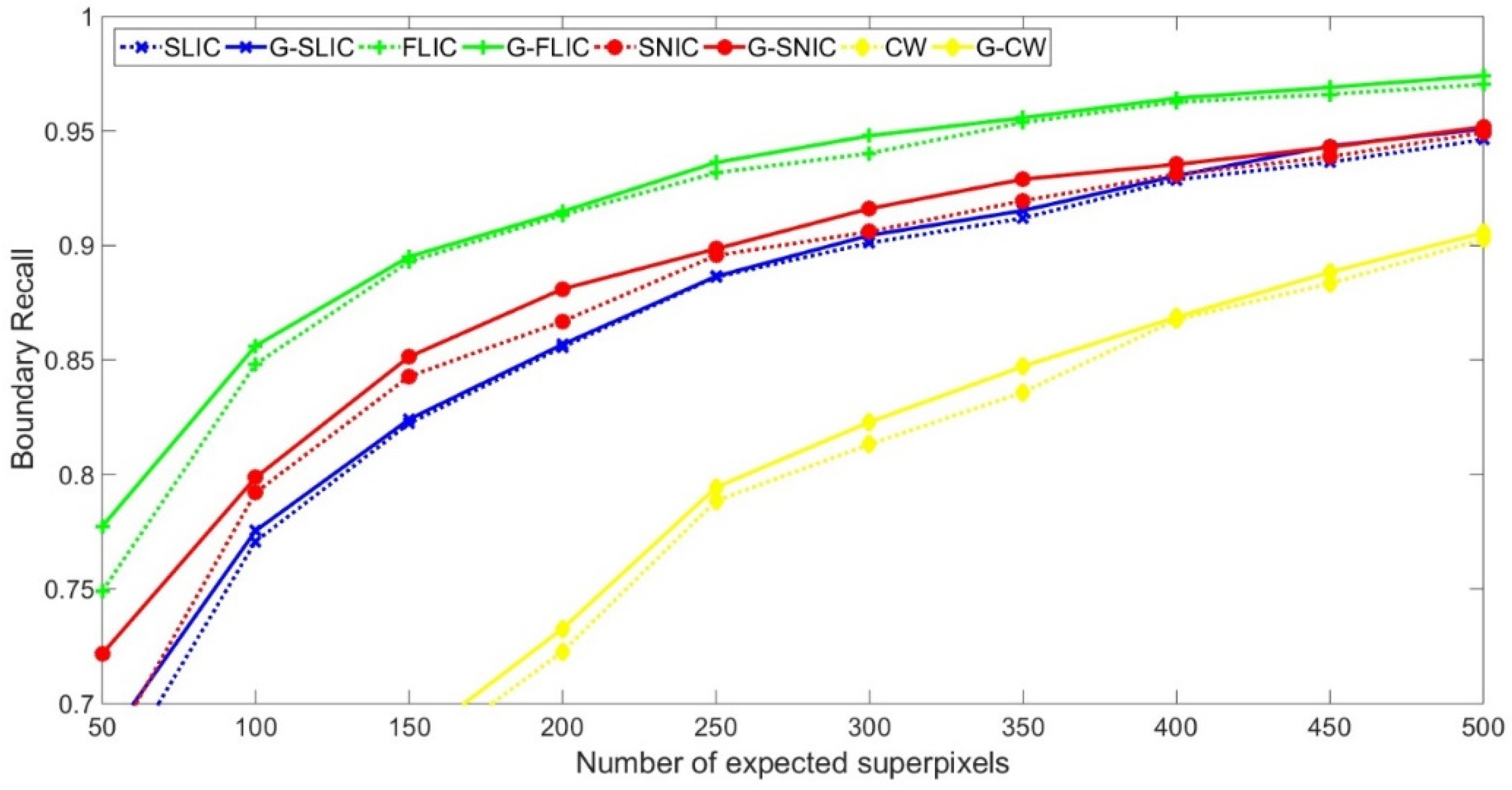
4.1. Quantitative Evaluation by Metrics

To objectively evaluate the performance with and without GRID in four algorithms, several evaluation metrics in the commonly used benchmark toolbox [32] are taken into account in this subsection. Mathematically, let Ω = { Ω k } k = 1 K and G = { G m } m = 1 M be the calculated superpixels and the ground truth of the same image { I i } i = 1 N , respectively. These metrics are defined as follows.
Boundary Recall (BR) is a typical boundary-detection and segmentation evaluation criterion on edge consistency. It is the ratio of ground truth boundaries covered by superpixel boundaries
BR = i G b B ( min j Ω b P ( I i ) P ( I j ) 2 < r ) G b ,
where Ω b and G b represent boundary pixels in Ω and G , respectively. B (   ) returns the boolean value whether the expression is true. The coverage radius r is set to 2 in this paper. Therefore, the higher the value of BR, the better boundary adherence the algorithm performs.
Figure 4 makes comparisons between reference algorithms and the corresponding improvements. It is clear that all the performance of GRID-embedded implementations upgrades, especially when the expected number is small. Nevertheless, there are still significant gaps among four pairs of algorithms. Theoretically in conventional SLIC, a minor distance in Equation (1) is acquired by comparing the value of a current pixel with the previous in a 2 S × 2 S region. Such a forward judgment easily leads to misclassification since some heterogeneous pixels might show relatively short distances at the beginning of local k-means clustering. Even the situation can be alleviated by repeated iterations, it results in inferior segmentation performance. In contrast, FLIC adopts an active search strategy to avoid the clusters being limited in a fixed range in space; the influence can be abated by absorbing more homogeneous pixels. It therefore achieves more acceptable boundary adherence than SLIC in a wider range of predicted superpixel numbers. Different from SLIC and FLIC, SNIC generates superpixel regions in a one-pass manner instead of iterative re-labeling in global scope, which also achieves a better performance. In CW, the compactness sometimes cumbers the adaption to object boundaries while it prevents the production of very large fragments. It does not work very attractively unless the amount of superpixels is high enough.
Under-segmentation Error (UE) measures how each superpixel overlaps with only one object
UE = m = 1 M ( Ω k | Ω k G m ϕ | Ω k | ) N N ,
where |   | means the number of pixels in a superpixel. Compared with BR, it utilizes segmentation regions instead of boundaries for measurement. For large superpixels, theoretically, there is a serious penalty if they have only a small overlap with the ground truth segment.
In Figure 5, for each algorithm, the value of UE decreases as the number of superpixels increases. Generally speaking, there is a contradiction between compactness and boundary adaption. Since the regular superpixels are more likely to straddle over multiple object regions [27], a strong compactness constraint leads to a downside of UE. Similar to BR, CW performs the worst on this metric when the number of superpixels is small. In another aspect, compared with the grid sampling initialization method, GRID promotes all four algorithms. It introduces color diversity as prior information so that all sub-regions are treated differently. Consequently, it is easier for complicated texture and small size regions to acquire sufficient initial seeds that catch more context information in detail.
Achievable Segmentation Accuracy (ASA) is introduced to quantify the accuracy achievable by subsequent steps, such as image segmentation and object recognition. Mathematically, ASA can be computed by
ASA = k = 1 K arg max m | Ω k G m | m = 1 M | G m | .
Similar to UE, it uses region information to evaluate the performance. A higher ASA value indicates that the subsequent performance of superpixels is unaffected.
Figure 6 further confirms the availability of the proposed strategy. Similar to BR and UE, with the growing number of superpixels, a GRID-embedded algorithm still outperforms the corresponding implementation without any initialization optimization. It also indicates that the GRID-based superpixels could prompt higher upper bounds of accuracy for subsequent visual tasks.
In addition to the three metrics listed above, the number of actual generated superpixels is introduced to determine the controllability to the number of superpixels. Table 2 illustrates the numerical comparison of superpixels between actual generation and user-expectation, which are produced by four algorithms on all test images in BSDS500 with and without GRID, respectively.
Apparently, SNIC and CW output a stable number of superpixels identical to the initialized seeds examined in Section 3.1. While the values are not exactly the same as the user’s expectation, they can be regarded as number-controllable methods based on the input. In contrast, the numbers of SLIC and FLIC are both without obvious rules due to the heuristic post-processing step that an isolated cluster is simply merged into its largest neighbor.
As presented in Algorithm 1, during the recursive modification process, the number of final seeds equals the length of the priority queue, wherein the sum of elements increases separately. Consequently, GRID initialization produces an exact number of superpixels expected by the user. The same quantity of superpixels is provided by SNIC and CW, respectively. Considering SLIC and FLIC, in Figure 1e,g, the new cell for a sub-divided seed shrinks to 2/3 along the direction of sub-division. This area ratio is determined by the approximation of clustering merely based on coordinate information in Equation (1). Thus the corresponding search region for the seed is 4 times the expansion of the new cell. Moreover, this paper selects partitions that contain the converged position of all seeds as the origins. As a result, other fragments are merged by these seeding partitions so that they meet an identical number of seeds initialized by GRID.

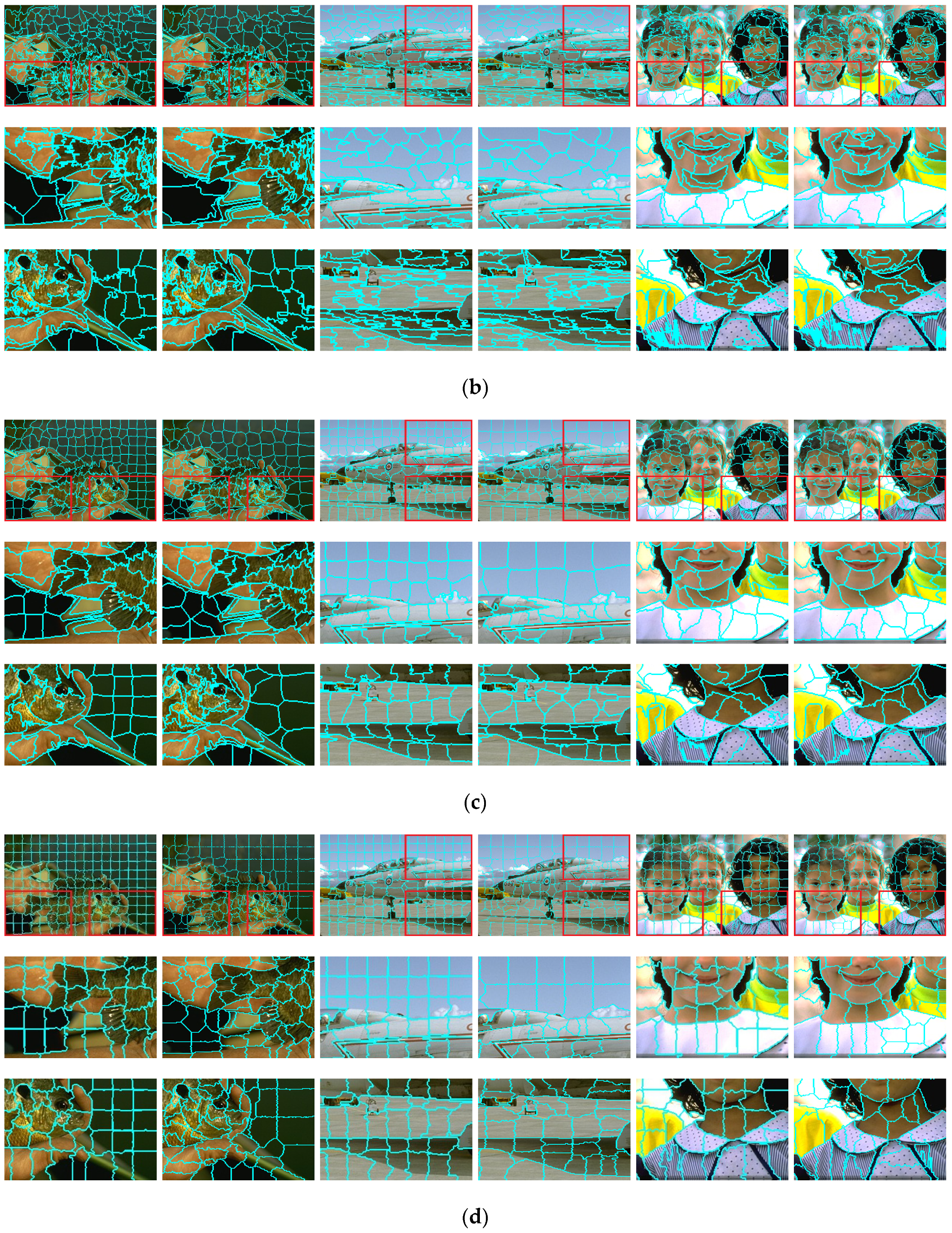
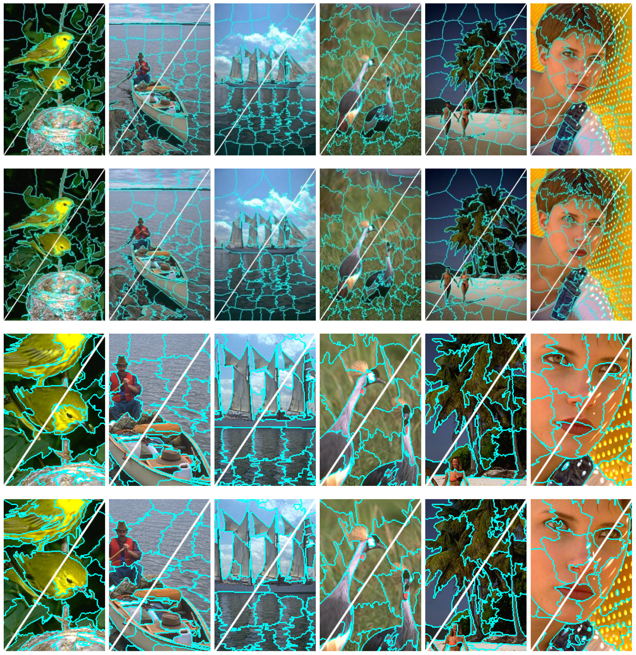
4.2. Visual Comparisons of Superpixel Results

For more insight into quantitative results, Figure 7 visualizes several segmentation results of the abovementioned superpixel algorithms for comparison. It can be observed in Figure 7d that CW fails to catch the boundaries accurately since the compactness constraint is too strong to conform to the image content. For example, most CW superpixels maintain rectangles approximately that result in heterogeneous fragments. Such under-segmentation is prone to miss the actual borders of different objects while their differences are very apparent. In contrast, G-CW overcomes this flaw by a series of recursive fission operations that generate new seeds with ideal initial positions. Consequently, it achieves finer-grained segmentation in the textured regions to some extent. More significant improvements can be revealed by G-SLIC as well as G-SNIC in Figure 7a,c. Both algorithms provide regular superpixels in size and shape, giving more attention to informative regions.
It is worth noting that, the proposed GRID initialization strategy could manipulate the seeds to cover slender objects, making them more accurate on twigs (e.g., red stripes on plane and black pattern on children). A particular condition is FLIC in Figure 7b, which is too sensitive to maintain compact outlines among neighboring superpixels, even if they all belong to a homogeneous region. While it achieves outstanding boundary adherence by sacrificing shape uniformity, it is desirable for G-FLIC to optimize the segmentation of low contrast regions. Due to sufficiently expected classes by multiple seeds, the cloud and plane in plane, as well as the chin and neck in children can be partitioned effectively although the difference is small.
More specifically, SNIC and G-SNIC are adopted to make additional visual comparisons. In Figure 8, G-SNIC superpixels maintain fine structures in accordance with the actual outlines of different objects. In addition, multi-scale representation of images that are smaller or larger in areas of high or low visual complexity is achieved. Therefore, the proposed GRID is capable of alleviating the contradiction that retains detail and keeps a moderate superpixel number simultaneously.

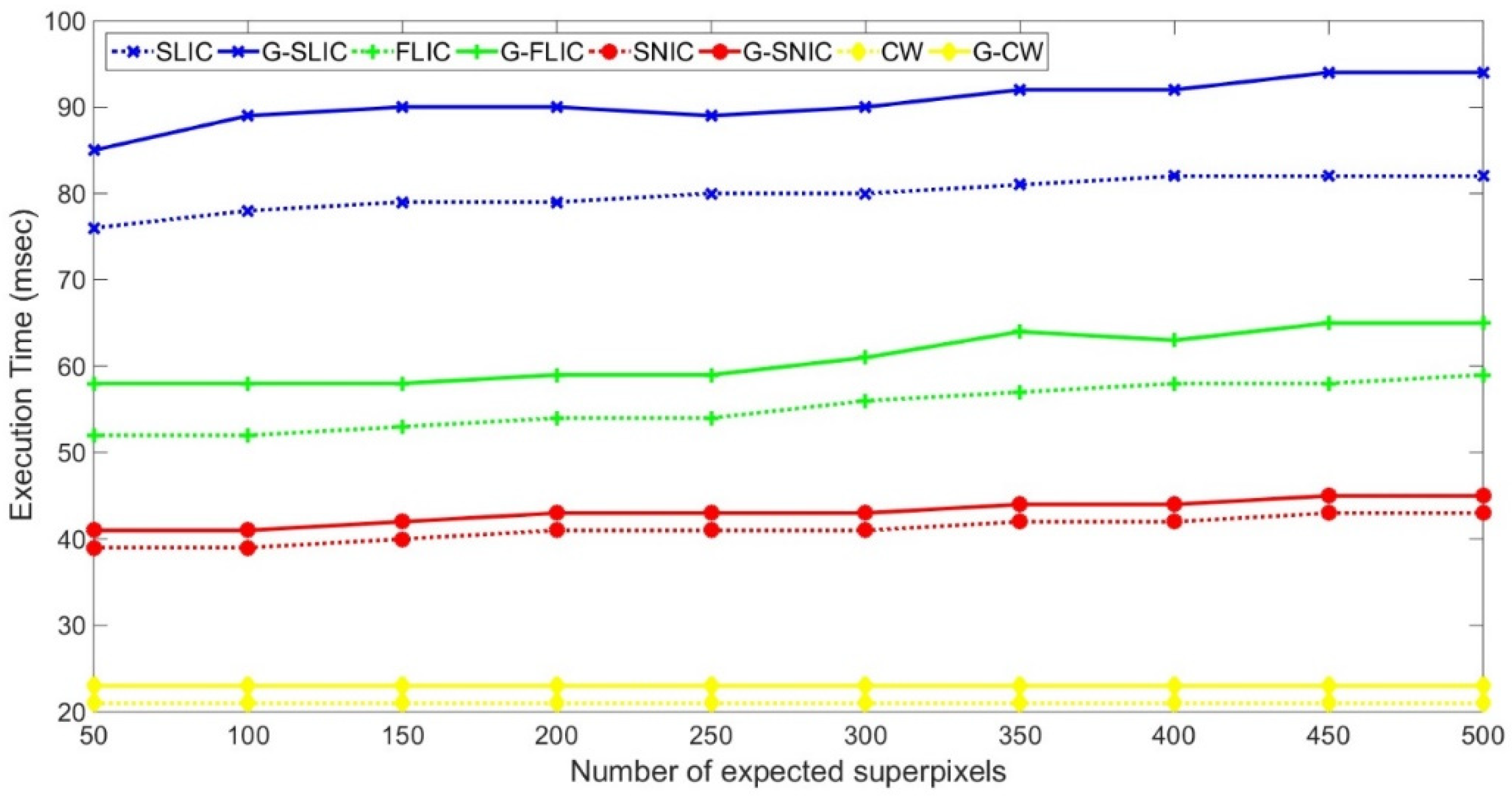
4.3. Analysis of Computational Efficiency

Execution Time (ET) is measured as the average runtime on the 200 test images on the BSDS 500. The available codes are all implemented in C++ and tested on an Intel Core i7-8550U CPU @ 1.80GHz with 16 GB RAM. Figure 9 demonstrates the comparison of ET on four pairs of conventional/GRID-embedded implementation, respectively. In principle, both FLIC and SNIC adopt a joint assignment and update strategy to address the delayed feedback from pixel label changes to superpixel seeds. This results in more rapid convergence than conventional SLIC that reaches an experientially predefined global termination. Unlike SNIC, where there is a redundant creation of neighboring elements, in CW, each pixel is inspected only once for the acquisition of the gradient image and the flooding. Therefore, it becomes the fastest among the four conventional methods. As an optimization of initialization, GRID slightly increases the runtime of all algorithms. In G-SNIC and G-CW, the increment appears to be irrelevant to the superpixel number. On the other hand, G-SLIC requires more time than the conventional implementation as well as G-FLIC, which shows fluctuation with the expectation.
A detailed discussion on the performance of time cost is presented in Table 3, with emphasis on 200 user-specified numbers of superpixels. All the algorithms consist of the two steps, initialization, assignment and updating, wherein SLIC/G-SLIC and FLIC/G-FLIC require an additional merging step as post-processing. Since the initialization of conventional grid sampling in Equation (8) is merely a numerical calculation, its time consumption can be omitted. The extra time consumed on GRID initialization is identical in all methods, and the additional 2 milliseconds are almost spent on establishing the SAT and relocating the new seeds. For G-SNIC and G-CW, the procedure of assignment and updating spends the same time as SNIC and CW, respectively. That is because both the two pairs of algorithms follow a non-iterative label expansion manner to cluster the superpixel regions in Figure 2. Therefore, the total computation is almost identical to a different number of expected superpixels. As a result, the disparity of time cost in this step is negligible when the difference of seeds (superpixels) number is very small in Table 2. Whereas in G-SLIC and G-FLIC, more seeds indicate that more 2 S × 2 S search regions need to be inspected. While the conventional SLIC and FLIC are both irrespective of seed number in theory, the additional inspection by GRID in Figure 1e–g costs an extra 9% and 4% time. Meanwhile, the optimized post-processing step mentioned in Section 4.1 also increases the time cost slightly. Overall, compared with the conventional methods, GRID-embedded implementation can be recognized as a balanced trade-off between runtime and accuracy. It also provides plug-and-play capability for several gradient-based superpixel methods with very minor modifications on the clustering procedure.

5. Conclusions

In this paper, a novel initialization strategy, GRID, is proposed to improve the performance of grid sampling-based superpixel segmentation algorithms. It follows a coarse-to-fine approach to recursively generating the initial seeds that are aware of the image content. Instead of straight distributing all seeds, half of the expected number of seeds is firstly located by the conventional initialization method. Thus, a coarse distribution of regional color information is established. It is then utilized as a reference for creating new seeds that lower the amount of color information in smaller ranges. Therefore, the distribution of recursively produced seeds is more sensitive to the complexity of regional information. Finally, the availability and efficiency of GRID is verified by embedding it into four superpixel segmentation algorithms and replacing the conventional grid sampling. Experimental results show that GRID-embedded algorithms acquire the controllability of outputting the exact number of superpixels expected by the user, with comparable quantitative metrics on the BSDS500 dataset.
In future research, it is worth exploring scale-adaptive superpixels, which could conform to the varying content of images more reasonably. Moreover, parameter-free algorithms are also required for advanced visual applications.

Author Contributions

All the authors contributed to this study. C.L.: investigation and writing of the original draft; B.G.: conceptualization, funding acquisition and project administration; Z.H. and J.G.: software and data curation; X.H.: resources; W.H.: supervision. All authors have read and agreed to the published version of the manuscript.

Funding

This research is supported financially by National Natural Science Foundation of China (Grant No. 61571346 and 51805398).

Acknowledgments

The authors would like to thank the editor and anonymous reviewers for their valuable comments on this paper.

Conflicts of Interest

The authors declare no conflict of interest.

References

  1. Ren, X.; Malik, J. Learning a classification model for segmentation. In Proceedings of the IEEE International Conference on Computer Vision (ICCV), Nice, France, 13–16 October 2003; pp. 10–17. [Google Scholar]
  2. Lee, K.; Sim, J. Warping Residual Based Image Stitching for Large Parallax. Proceedings of the Computer Vision and Pattern Recognition (CVPR). Available online: http://cvpr20.com/ (accessed on 25 July 2020).
  3. Yeo, D.; Son, J.; Han, B.; Han, J. Superpixel-based tracking-by-segmentation using Markov chains. In Proceedings of the Computer Vision and Pattern Recognition (CVPR), Honolulu, HI, USA, 21–26 July 2017; pp. 511–520. [Google Scholar]
  4. Spampinato, C.; Palazzo, S.; Giordano, D. Gamifying video object segmentation. IEEE Trans. Pattern Anal. Mach. Intell. 2017, 39, 1942–1958. [Google Scholar] [CrossRef] [PubMed] [Green Version]
  5. Lu, H.; Li, X.; Zhang, L.; Ruan, X.; Yang, M. Dense and sparse reconstruction error based saliency descriptor. IEEE Trans. Image Process. 2016, 25, 1592–1603. [Google Scholar] [CrossRef] [PubMed]
  6. Chen, J.; Hou, J.; Ni, Y.; Chau, L. Accurate light field depth estimation with superpixel regularization over partially occluded regions. IEEE Trans. Image Process. 2018, 27, 4889–4900. [Google Scholar] [CrossRef] [PubMed] [Green Version]
  7. Stutz, D.; Hermans, A.; Leibe, B. Superpixels: An evaluation of the state-of-the-art. Comput. Vis. Image Underst. 2018, 166, 1–27. [Google Scholar] [CrossRef] [Green Version]
  8. Shi, J.; Malik, J. Normalized cuts and image segmentation. IEEE Trans. Pattern Anal. Mach. Intell. 2000, 22, 888–905. [Google Scholar]
  9. Grady, L. Random walks for image segmentation. IEEE Trans. Pattern Anal. Mach. Intell. 2006, 28, 1768–1783. [Google Scholar] [CrossRef] [Green Version]
  10. Liu, M.; Tuzel, O.; Ramalingam, S.; Chellappa, R. Entropy rate superpixel segmentation. In Proceedings of the IEEE Conference on Computer Vision and Pattern Recognition (CVPR), Colorado Springs, CO, USA, 20–25 June 2011; pp. 2097–2104. [Google Scholar]
  11. Shen, J.; Du, Y.; Wang, W.; Li, X. Lazy random walks for superpixel segmentation. IEEE Trans. Image Process. 2014, 23, 1451–1462. [Google Scholar] [CrossRef]
  12. Kang, X.; Zhu, L.; Ming, A. Dynamic random walk for superpixel segmentation. IEEE Trans. Image Process. 2020, 29, 3871–3884. [Google Scholar] [CrossRef]
  13. Achanta, R.; Shaji, A.; Smith, K.; Lucchi, A.; Fua, P.; Susstrunk, S. SLIC superpixels compared to state-of-the-art superpixel methods. IEEE Trans. Pattern Anal. Mach. Intell. 2012, 34, 2274–2282. [Google Scholar] [CrossRef] [Green Version]
  14. Vincent, L.; Soille, P. Watersheds in digital spaces: An efficient algorithm based on immersion simulations. IEEE Trans. Pattern Anal. Mach. Intell. 1991, 13, 583–598. [Google Scholar] [CrossRef] [Green Version]
  15. Giraud, R.; Ta, V.; Papadakis, N. Robust superpixels using color and contour features along linear path. Comput. Vis. Image Underst. 2018, 170, 1–13. [Google Scholar] [CrossRef] [Green Version]
  16. Liu, Y.; Yu, M.; Li, B.; He, Y. Intrinsic manifold SLIC: A simple and efficient method for computing content-sensitive superpixels. IEEE Trans. Pattern Anal. Mach. Intell. 2018, 40, 653–666. [Google Scholar] [CrossRef] [PubMed]
  17. Zhao, J.; Hou, Q.; Ren, B.; Cheng, M.; Rosin, P. FLIC: Fast linear iterative clustering with active search. In Proceedings of the AAAI Conference on Artificial Intelligence (AAAI), New Orleans, LA, USA, 2–7 February 2018; pp. 7574–7581. [Google Scholar]
  18. Achanta, R.; Susstrunk, S. Superpixels and polygons using simple non-iterative clustering. In Proceedings of the IEEE Conference on Computer Vision and Pattern Recognition (CVPR), Honolulu, HI, USA, 21–26 July 2017; pp. 4895–4904. [Google Scholar]
  19. Huang, C.; Wang, W.; Wang, W.; Lin, S.; Lin, Y. USEAQ: Ultra-fast superpixel extraction via adaptive sampling from quantized regions. IEEE Trans. Image Process. 2018, 27, 4916–4931. [Google Scholar] [CrossRef] [PubMed]
  20. Hu, Z.; Zou, Q.; Li, Q. Watershed superpixel. In Proceedings of the IEEE International Conference on Image Processing (ICIP), Quebec City, QC, Canada, 27–30 September 2015; pp. 349–353. [Google Scholar]
  21. Neubert, P.; Protzel, P. Compact Watershed and Preemptive SLIC: On improving trade-offs of superpixel segmentation algorithms. In Proceedings of the IEEE International Conference on Pattern Recognition (ICPR), Stockholm, Sweden, 24–28 August 2014; pp. 996–1001. [Google Scholar]
  22. Machairas, V.; Faessel, M.; Cardenas, D.; Chabardes, T.; Walter, T.; Decencière, E. Waterpixels. IEEE Trans. Image Process. 2015, 24, 3707–3716. [Google Scholar] [CrossRef] [Green Version]
  23. Xiao, X.; Zhou, Y.; Gong, Y. Content-adaptive superpixel segmentation. IEEE Trans. Image Process. 2018, 27, 2883–2896. [Google Scholar] [CrossRef]
  24. Xu, L.; Luo, B.; Pei, Z.; Qin, K. PFS: Particle-filter-based superpixel segmentation. Symmetry 2018, 10, 143. [Google Scholar] [CrossRef] [Green Version]
  25. Lloyd, S. Least squares quantization in PCM. IEEE Trans. Inf. Theory 1982, 28, 129–137. [Google Scholar] [CrossRef]
  26. Du, Q.; Faber, V.; Gunzburger, M. Centroidal Voronoi tessellations: Applications and algorithms. SIAM Rev. 1999, 41, 637–676. [Google Scholar] [CrossRef] [Green Version]
  27. Li, C.; Guo, B.; Wang, G.; Zheng, Y.; Liu, Y.; He, W. NICE: Superpixel segmentation using non-iterative clustering with efficiency. Appl. Sci. 2020, 10, 4415. [Google Scholar] [CrossRef]
  28. Meyer, F. Color image segmentation. In Proceedings of the International Conference on Image Processing (ICIP), Singapore, 7–11 September 1992; pp. 303–306. [Google Scholar]
  29. Achanta, R.; Marquez, P.; Fua, P.; Susstrunk, S. Scale-adaptive superpixels. In Proceedings of the IS&T Color and Imaging Conference (CIC), Vancouver, BC, Canada, 12–16 November 2018; pp. 1–6. [Google Scholar]
  30. Viola, P.; Jones, M. Rapid object detection using a boosted cascade of simple features. In Proceedings of the IEEE Conference on Computer Vision and Pattern Recognition (CVPR), Kauai, HI, USA, 8–14 December 2001; pp. 511–518. [Google Scholar]
  31. Arbelaez, P.; Maire, M.; Fowlkes, C.; Malik, J. Contour detection and hierarchical image segmentation. IEEE Trans. Pattern Anal. Mach. Intell. 2011, 33, 898–916. [Google Scholar] [CrossRef] [Green Version]
  32. Wang, M.; Liu, X.; Gao, Y.; Ma, X.; Soomro, N. Superpixel segmentation: A benchmark. Signal Process. Image Commun. 2017, 56, 28–39. [Google Scholar] [CrossRef]
Figure 1. The schematic diagram of the proposed GRID initialization method. (a) Input image; (b) Summed area table corresponding to the lightness channel of (a); (c) Grid sampling initialization with half the expected number of seeds; (d) The ordered distribution of color information for all rectangular cells of (c), and the sub-region surrounded by a yellow rectangle containing the maximum information. For visualization, the values are normalized in the range of 0 to 255 as well as (b); (eg) Zoom-in GRID performance of (d), which are performed recursively till the expected superpixel number is obtained. (h) The result of superpixel segmentation. The black dotted rectangle and circle denote the region with maximum information and corresponding initial seed, respectively. The color solid rectangles and filled circles denote the sub-regions and the sub-divided seeds that balance the information to a certain extent. A black filled circle represents that the amount of information in the corresponding sub-region is not the most in the current loop. It is likely to be sub-divided after several rounds of global sorting of the regional information amount.
Symmetry 12 01417 g001
Figure 2. Dynamic segmentation procedure of two patterns of grid sampling-based algorithms to generate superpixels. (a) Initialization of the input image. (b) Assignment and updating of clusters. (c) The resulting superpixels. In (b,c), the strategies of iterative label updating and non-iterative label expansion are filled with yellow and cyan. For simplicity, the merging step is omitted in yellow.
Symmetry 12 01417 g002
Figure 3. Sample grids against different excepted numbers of superpixels over a 481 × 321 image in black. (a) The actual cell number is 150, identical to the expectation. (b) The actual cell number is 187, less than the expectation of 200. (c) The actual cell number is 260, more than the expectation of 250. Note that cells at the right and lower sides are not squares because of the deviation by floor operations.
Symmetry 12 01417 g003
Figure 4. Comparison of four pairs of algorithms in terms of boundary recall. Some curves are truncated for better visual contrasts.
Symmetry 12 01417 g004
Figure 5. Comparison of four pairs of algorithms in terms of under-segmentation error.
Symmetry 12 01417 g005
Figure 6. Comparison of four pairs of algorithms in terms of achievable segmentation accuracy.
Symmetry 12 01417 g006
Figure 7. Visual comparison of fish, plane and children among four different methods with and without GRID initialization in alternating columns. (a) SLIC; (b) FLIC; (c) SNIC; (d) CW. Each segmented image is generated by nearly and exactly 200 superpixels, followed by two zoom-in results of local regions enclosed by red rectangles.
Symmetry 12 01417 g007aSymmetry 12 01417 g007b
Figure 8. Visual comparison of segmentation results with zoom-in performance. The first two rows display SNIC and G-SNIC, respectively, and the last two rows show the corresponding central details. In each image, the expected superpixel number in the upper left and lower right is 50 and 100, respectively.
Symmetry 12 01417 g008
Figure 9. Comparison of execution time (msec) in the proposed four pairs of algorithms on BSDS500.
Symmetry 12 01417 g009
Table 1. Key notations used in this paper. Notice that symbols are specified by the bold letters corresponding to the real meanings.
NotationDefinition
F ( I i ) The 5-dimensional Feature vector of the i th element I i in an image I = { I i } i = 1 N
C ( I i ) The Color vector of I i in a 3-channel CIELAB image space consisting l, a and b
P ( I i ) The Position vector of I i in a 2-dimensional Euclidean space consisting x and y
p ( I i ) The priority of pixel I i in a watershed-based algorithm
{ s k } k = 1 K The set of excepted K seeds in image I = { I i } i = 1 N
{ s k ¯ } k = 1 K The updated set of excepted K seeds { s k } k = 1 K
S = N / K The Step size of regular cells in the image grid
D ( I m , I n ) A joint spatial–color Euclidean Distance between I m and I n in a image plane
L ( I i ) The final Label assigned to I i by a superpixel algorithm
f ( C ; μ , σ ) The probability function of color in a multivariate double exponential distribution
T ( Ω k ) The Total information contained in a superpixel region Ω k
A ( k ) The Amount of color information in k th cell k
S A T ( x , y ) The value of an element ( x , y ) in a Summed Area Table
Table 2. Comparison of superpixel number between user-expectation and actual generation.
User-Expected Superpixel NumberNumber of Superpixels Generated by Algorithms without GRID Initialization (SLIC/FLIC/SNIC/CW)GRID-Based Superpixel Number
Min NumberMean NumberMax Number
5028/33/40/4041/45/40/4050/67/40/4050/50/50/50
10069/78/96/9692/101/96/96114/131/96/96100/100/100/100
150107/119/150/150143/156/150/150168/204/150/150150/150/150/150
200145/156/187/187185/198/187/187223/257/187/187200/200/200/200
250198/190/260/260252/243/260/260300/309/260/260250/250/250/250
300235/221/294/294289/280/294/294354/349/294/294300/300/300/300
350259/272/330/330324/347/330/330379/425/330/330350/350/350/350
400323/310/400/400394/401/400/400452/493/400/400400/400/400/400
450367/331/442/442436/426/442/442487/539/442/442450/450/450/450
500408/363/504/504496/472/504/504554/595/504/504500/500/500/500
Table 3. Comparison of time cost (msec) in the proposed four pairs of algorithms with K = 200 .
AlgorithmInitializationAssignment and UpdatingPost-ProcessingTotal Execution Time
SLIC-77279
G-SLIC284490
FLIC-48553
G-FLIC250658
SNIC-41-41
G-SNIC241-43
CW-21-21
G-CW221-23

