1. Introduction
Future wireless networks should not only realize communication, but also support new services, such as connected transportation systems, smart logistics, unmanned factories, etc. [
1,
2,
3,
4]. As one of the enabling techniques, position detection is becoming increasingly important. Its technical evolution can be found in discussions within the Third-Generation Partnership Project (3gpp), the Bluetooth Special Interest Group (SIG), and other standard development organizations. Such applications should not only be confined to two-dimensional (2D) planes, but also be implementable to three-dimensional (3D) spaces.Moreover, communication may also rely on positioning techniques. For example, in multiple-input multiple-output (MIMO) systems, beamforming is well utilized to focus the signal power towards a specified receiver. However, conventional approaches for deciding the beam direction may not satisfy the future requirement, especially when the target is moving. Hence, a robust and low-complexity tracking solution should be considered.
To track non-linear target movement in practice, the extended Kalman filter (EFK) is used. One of the factors that influences the accuracy of EKF is the variance estimation of observation errors [
5,
6]. In this paper, the observation process in EKF is realized by a specific location detector, instead of a theoretical model in many previous works [
7,
8]. Usually, it is difficult to estimate the variance of detection errors in real-time scenarios. Such estimation may get even worse when the environment changes. For example, in connected car networks, car sensing may not only be performed by fixed infrastructures on the roads, but also be conducted by surrounding vehicles, which forms a simultaneous localization and mapping (SLAM) problem [
9,
10]. In SLAM, the sensing environment may change as devices move, and the variance of detection errors may become unstable. Hence, it is a crucial challenge for the tracking system to perform accurate estimations of such variance in real time.
In SLAM, multiple sensors can be used for detecting a single target. Actually, since the network density continues to grow, the utilization of multiple distributed sensing devices will become more convenient in the future. Therefore, this paper considers a scenario with distributed sensors. To perform a location detection with distributed sensors, many algorithms have been proposed. For example, in [
11], the least squares (LS) method was applied for indoor positioning, and a hybrid system combining time-difference-of-arrival (TDOA) and angle-of-arrival (AOA) measurements was considered. In [
12], a factor-graph (FG) method [
13] was proposed for location detection using time-of-arrival (TOA) measurement. The performance was shown to achieve the maximum likelihood (ML) bound with relatively low complexity. Due to such advantages, many extensions of the FG algorithm to other applications can be found in [
14,
15,
16] for received-signal-strength (RSS), TDOA, and AOA, respectively. This work will also focus on FG for both location detection and tracking.
A location detection and tracking algorithm using TOA was proposed in [
17]. However, the use of TOA always requires strict time synchronization, because the signal emitting time should be known. Such a limitation will increase the difficulties of implementing such a technique in practice. Moreover, for an anonymous target that may not provide any transmission information to sensors or the fusion center, TOA cannot be used. There are still some limitations for RSS-based detection [
14]. For example, RSS is also regarded as a technique only for a known target, because the training of received signal strength has to be conducted before the real deployment. To deal with the drawbacks mentioned above, TDOA-based techniques can be used, which does not require synchronization between the target and sensors, as well as off-line training. However, the performances are too sensitive to the measurement errors, due to the light speed.
In contrast, the performances of AOA-based techniques are not so sensitive to measurement errors, while still enjoying the same advantages as TDOA for detecting anonymous targets. Therefore, this paper will focus on AOA. In [
16,
18,
19], AOA-based location detection and tracking was studied. However, the previous works only considered the scenarios in 2D. Actually, the use cases in 3D are currently increasing. For example, it can be applied to aviation control for airports, where not only the scheduled aircraft, but also the anonymous invaders can be detected and tracked. Moreover, live TV broadcasts via cameras on drones will become more popular, which requires accurate drone control in 3D by the fusion center. Additionally, future intelligent transportation systems may realize 3D detection capability to assist the navigation of vehicles running in the complex multi-layer overpass roads. Note that the measurement of AOA samples, including azimuth and elevation angles in 3D, may require more complicated soft/hard designs, such as MUSIC and ESPRIT [
20,
21], but they are out of the scope of this paper.
For location detectors that work in a relatively stable condition, the variance of detection errors will also be stable. In this case, a fixed variance value can be fed to EKF for estimating the performance of the observer. Usually, such a value can be calculated from off-line training. However, this paper considers a dynamic system, which indicates that the measuring abilities of sensors may vary through the tracking process. Therefore, a real-time tuning approach of the observation variance is required. This paper proposes an estimation method by using an approximated Cramer–Rao bound (ACRB). Specifically, the Cramer–Rao bound (CRB) provides a low bound on the detection performance according to the measurement of indirect parameters. For the AOA-based location detection problem, the CRB can be calculated by using the variances of AOA measurements and the real position of the target. However, the latter parameter is unavailable in practice. Instead, it is possible to get a predicted target position with EKF, with which the ACRB can be calculated as the estimation of the observation variance. Such a process can work in dynamic environments and has been shown to achieve a robust tracking performance in this paper.
The main contribution of this paper can be summarized as follows.
An integrated FG structure is formulated to realize 3D location detection and tracking with AOA measurements.
It has been proven that the information from the elevation angle can help to improve the detection of 2D space, from both theoretical and simulation analyses.
The proposed technique has exhibited robust performances even with an unstable sensing environment.
By utilizing the ACRB as side information (SI) to the detector, the proposed system can greatly reduce the impacts of burst sensing errors.
The organization of this paper is as follows. The proposed system model is described in
Section 2. Then, the proposed FG algorithms for realizing the location detector and tracking are provided in
Section 3 and
Section 4, respectively. After that, the derivations of CRB and ACRB are given in
Section 5. The simulation results that prove the superiority of the proposed technique are provided in
Section 6. Finally, the conclusion is given in
Section 7 with some remarks.
2. System Model
In this paper, a discrete and non-linear state space model (SSM) is considered. A single target is to be detected, and its state at time index
k can be denoted by the 3D location
, with
. Moreover, there are
N distributed sensors deployed in this system, and the fusion center is assumed to know their position
, with
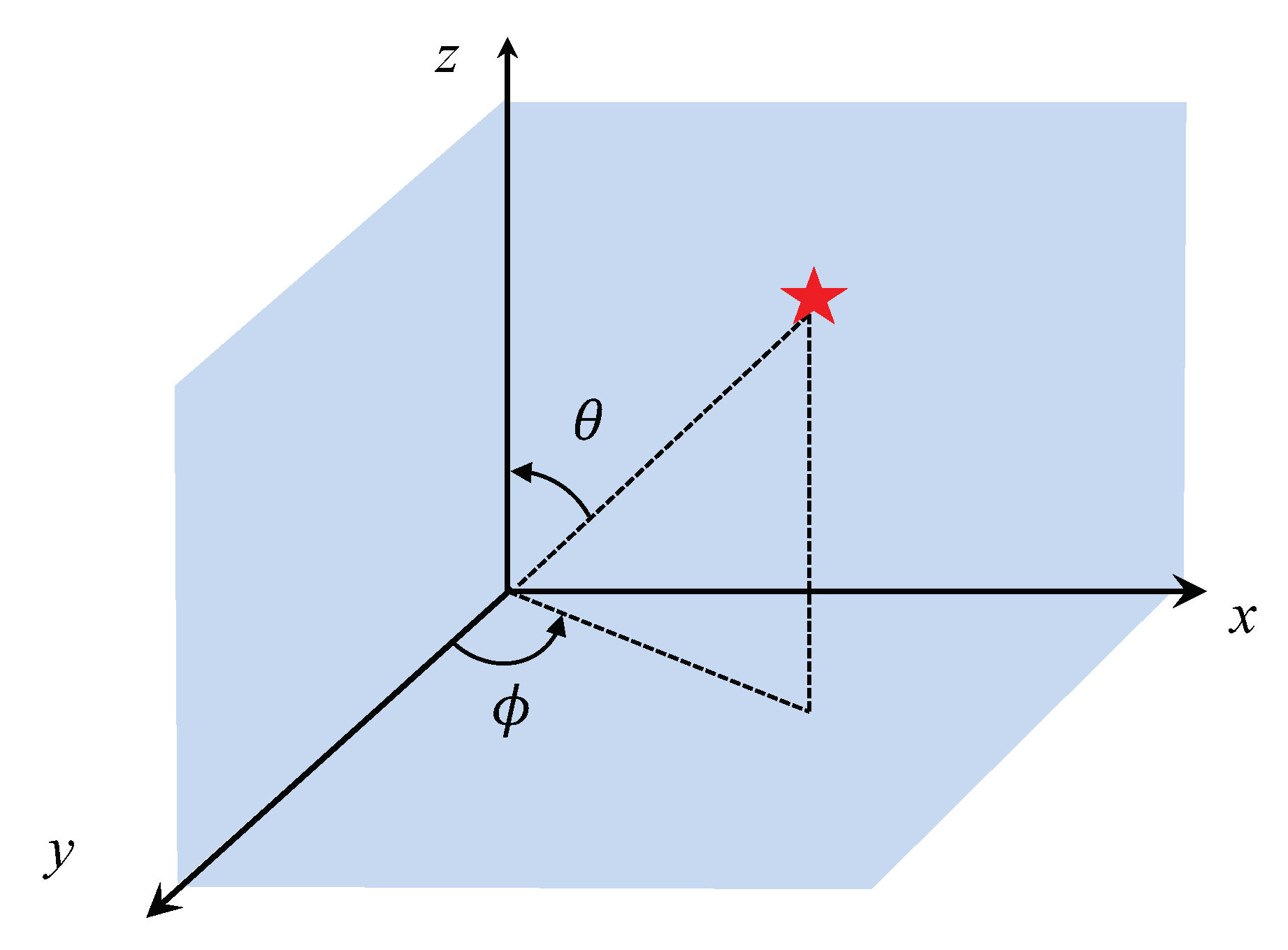
. The azimuth and elevation angles, denoted by
and
, respectively, are shown in
Figure 1. For the sake of performing location detection, the relative distance
from the
n-th sensor to the target is computed by:
The measured AOA at each sensor is comprised of both azimuth
and elevation
angles. The definition of
and
in the spherical coordinate exactly follows the standard way shown in
Figure 1. The relative distances calculated above can be connected by the true AOAs as follows, where the subscripts are omitted for simplicity.
As shown in Equations (
3)–(
6), the calculations of relative distances are self-contained. In order to obtain a converged result, iterative detection is performed based on an FG framework, which is known as the message passing algorithm. Note that there are always two ways to calculate the relative distance, which indicates that there will be two factor nodes included in the proposed FG structure, connecting to the variable node of the relative distance. A detailed discussion of the FG structure will be given in the next section. Moreover, it is assumed that for every time index, sensors are able to measure
L samples of AOA from the target, and the variable of measured AOA can be described as a Gaussian model as:
where
, and the noise components
and
follow
and
, respectively. Even though the quantization errors may break the Gaussianity of the measured AOAs, they are assumed to be very small in this paper, such that the input of the FG detector can be still regarded as Gaussian distributed variables. Moreover, it is assumed that the measured AOAs can be sent from sensors to the fusion center with error-free transmissions. Due to the Gaussian assumption of the measured AOAs at each sensor, they can be described by only parameters of the Gaussian probability density function (PDF), instead of
L snapshots. By omitting the indexes
n and
k for simplicity,
and
are used to represent the mean and the variance of
, respectively. Similarly,
and
are used to represent the mean and the variance of
, respectively. Clearly, when
L becomes larger, the means and variances obtained from AOA measurements will be closer to the real values.
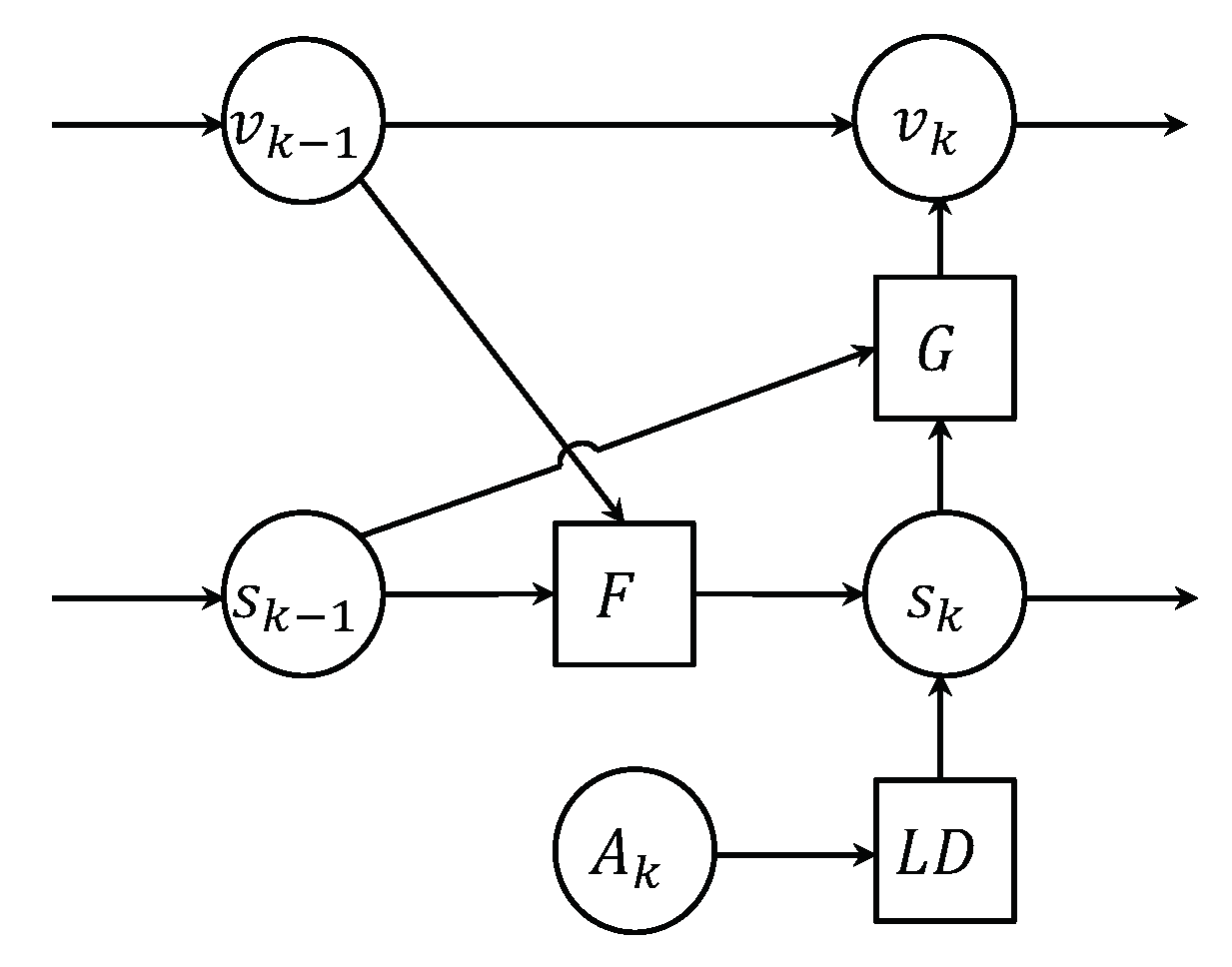
To describe the tracking model, the state process equation in EKF is first given by:
where
denotes the noise vector, and each of the elements follows a Gaussian distribution with
. As a non-linear function,
determines the movement of the target. To realize EFK, the conventional way is to approximate
linearly by
, according to the Taylor expansion of the first order. Unfortunately, in this paper, the target’s movement is unknown, which should be dynamically adjusted at each time index. Therefore, this work introduces an
such that
holds. Therefore, (
10) can be expressed by:
where
, known as the adjustment term, which should be updated dynamically at every time of the tracking process. Obviously, the accuracy of such a model can be guaranteed only if the target does not move far between two adjacent time indexes. Then, the observation equation can be also expressed as a function of the real target state, as:
where the observation noise vector is represented by
. Since
is fully determined by the true AOAs
and
,
can be also expressed by
. Note that
is not theoretically formulated in this paper, but realized by a practical 3D location detector. Within the proposed FG structure, all messages passed through are approximated to be Gaussian, including the noise of observation. Therefore, it is assumed that each element from
follows
. Unfortunately,
, which is needed to perform EKF, cannot be directly measured at the sensors. The theoretical bound of the observation result is determined by the CRB. In other words, the smallest achievable
can be calculated based on the variances of AOA measurements.
3. Location Detector
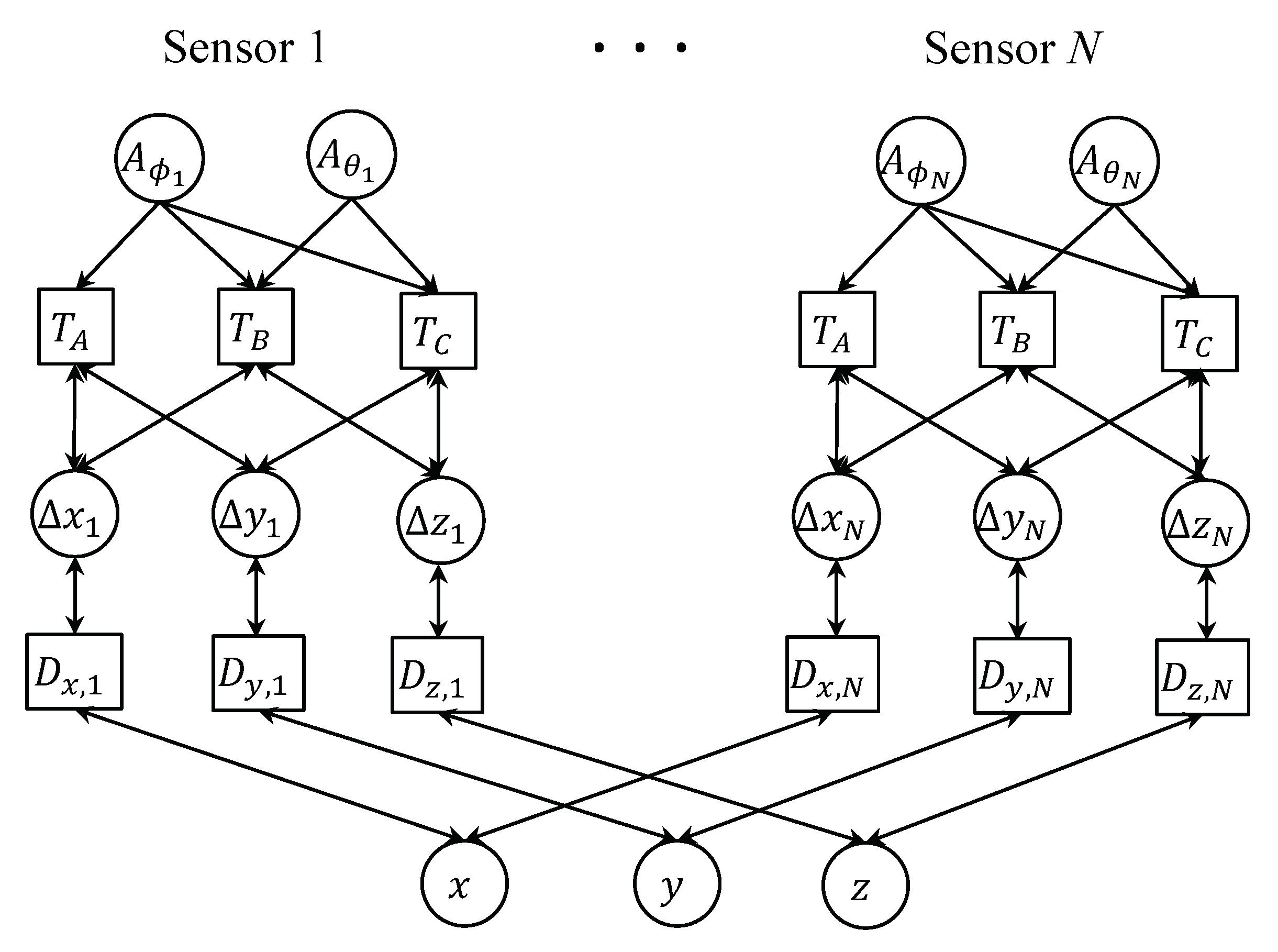
This section introduces the FG structure in detail for AOA-based 3D location detection, as shown in
Figure 2. It is also known as the observer in EFK. Note that in the following discussion, the indexes of the sensor are ignored from the variables for an easier expression. First of all, the variable nodes (
,
) are used, which contain the means and variances of the measured AOAs at each sensor. The outputs of (
,
), i.e., (
,
) and (
,
), are then sent to the factor nodes (
,
,
) for trigonometric calculations, which triggers the FG iterations.
As shown in
Figure 2,
only takes the information from
and then feeds its outputs to the variable nodes
and
, which forms a completed 2D location detection as in [
16]. The calculations within the factor node
are referred to (
3) and (
5). In order to further fulfill 3D location detection, the information from
should also be utilized. Therefore, factor nodes
and
are introduced, which connect both
and
and feed to (
,
) and (
,
), respectively. The operations within
and
are based on (
2), (
4), (
6), and (
7). As a result, each of the relative distance variables is linked to two different trigonometric factor nodes, as shown in
Figure 2.
It should also be noted that in , the multiplication of two independent Gaussian variables is needed, while in and , the multiplication of three independent Gaussian variables is required. Then, the means and variances of such multiplication results have to be calculated, assuming all messages are Gaussian.
Specifically, given two independent variables
and
, the product
can be expressed by the mean and the variance as:
If a third variable
is introduced, the product of them
can be expressed in a similar way, as:
However, the original trigonometric calculations shown in (
3)–(
6) are not linear, which may break the Gaussianity of the output of the factor nodes. To deal with this problem, the first order TSexpansion is used to approximate the non-linear function
as:
where the linear approximation is assumed to be around
. As a result, three constant values
,
, and
are obtained. Based on (
17), the approximated mean and variance of
can be expressed by:
Based on (
18) and (
19), it is straightforward to calculate the means and the variances of particular trigonometric functions of (
3)–(
6), which are summarized in
Table 1.
Given the mathematical preliminaries above, the proposed FG detection will be explained in detail as follows. First of all, messages containing means and variances of the measured AOAs will be fed to the trigonometric factor nodes
,
, and
. After that, the output messages go to relative distance variable nodes
,
, and
. As can be seen in
Figure 2, each of the relative distance variable nodes connect to two trigonometric factor nodes, which requires the multiplication of two independent Gaussian PDFs as,
Based on (
20), particular calculations of the means and variances of the iterative messages are made possible, from the relative distance variable nodes to the relative distance factor nodes, which are expressed by,
and:
On the other hand, the means of messages passing from the trigonometric factor nodes to the relative distance variable nodes are calculated as:
In addition, the variances passing from the factor node
to the variable node
can be calculated by:
and the variance passing from the factor node
to the variable node
is given by:
However, calculating the rest of the variances required in the proposed FG detection is omitted, due to the limited space. Actually, the way of such calculation is very similar to (
33) and (
34). Even though many calculations are involved in the equations mentioned above, some of them are reusable, which guarantees a low implementation complexity.
Finally, according to (
1), messages passing from the factor nodes of a relative distance to different axes can be expressed by:
and:
In the equations shown above, the variable subscripts indicating the sensor index are ignored for simplicity, because such steps are conducted for all sensors in parallel. At the variable nodes of estimated target position, messages coming from different sensors will be exchanged in order to make the FG iteration work. Therefore, the variable subscripts indicating the sensor index will be used when calculating the means and variances, as [
13]:
According to the design of real systems, the FG iteration can be performed until some particular conditions are satisfied. For example, if the gap of detected positions between two adjacent time indexes is less than a pre-defined threshold, or the maximum allowed iteration number is simply reached, the FG iteration can stop. Finally, the target location detected by the observer can be obtained by (
50)–(
52), where
,
, and
are calculated by (
47)–(
49), respectively.
6. Results
In this section, simulation results are provided in order to prove the accuracy, convergence, and robustness of the proposed technique. The real path of the moving target is formulated by functions with regard to the time index
k, as:
where
and
indicating the initial location. According to the specific simulation scenarios, the setting of sensor positions, FG iteration time, and AOA measurement variances will be different.
6.1. Accuracy Evaluation
In this subsection, the accuracy of the proposed tracking technique is evaluated by simulations. Three distributed sensors are deployed on the ground, with the positions at
,
, and
, respectively. Such a deployment is only based on practical considerations. Actually, the optimal sensor location cannot be guaranteed due to the mobility of the target, as in (
65) and (
66). The FG iteration number of the detector is fixed at 15, and 100 snapshots are assumed for the detection of each time index.
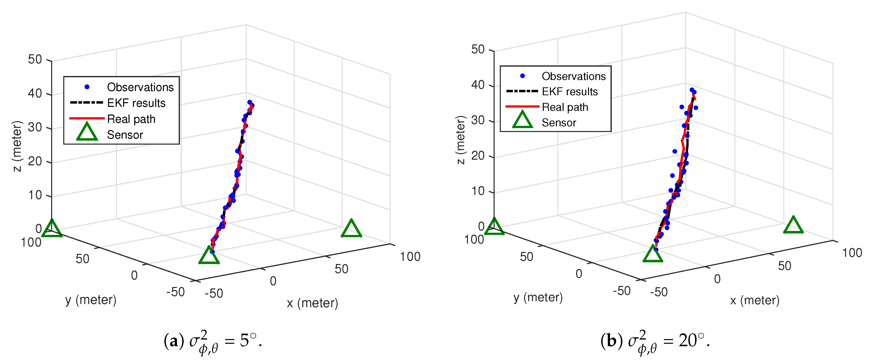
First of all, the real path of the target and tracking trajectories are shown in
Figure 4. Note that the standard deviations of AOAs from both the azimuth and elevation angles are set equal in the simulations, denoted by
, in order to evaluate the general tendency of the system behavior. However, in practice,
and
can be different. The tracking results with
can be seen in
Figure 4a. In order to evaluate the accuracy of the proposed tracking technique, RMSEs are calculated. Specifically, the observer, realized by the 3D location detector described in
Section 3, achieves RMSE = 1.6 meters, while this value is reduced to 1.4 with the proposed EKF. The RMSE values of the observer and the EKF are 6.15 and 4.6 in
Figure 4b, which are higher than
Figure 4a, because of a larger
is assumed in the simulation.
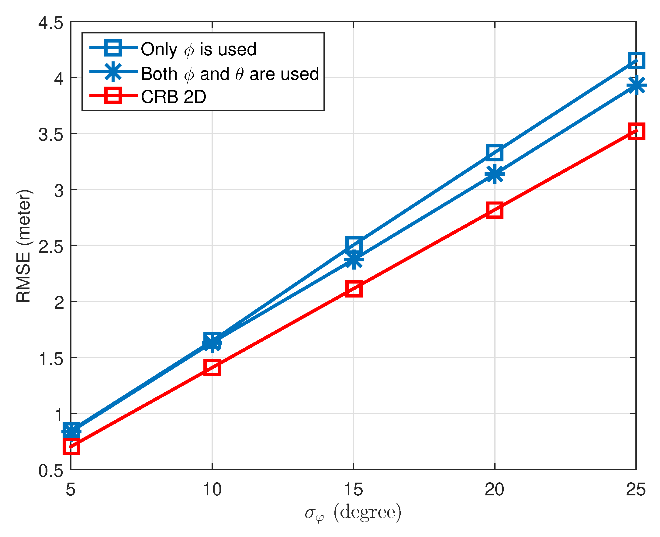
Moreover, another simulation was conducted to evaluate whether the 2D tracking performance can be improved with the help of the measured elevation angles. Actually, in many applications, the importance of 2D location accuracy is more than that of 3D. Therefore, it will be very beneficial to see if the 2D detection can be enhanced with additional assistance from elevation measurement. As shown in
Figure 5, the RMSE values achieved by using only the azimuth angle
for 2D detection are plotted, versus the standard deviation
. Interestingly, considering both
and
with 3D detection, the RMSEs in 2D are found smaller than the case where only
is used, which are closer to the theoretical CRB bound. This finding proves the fact that the information carried by the elevation angle
also contributes to the detection in the 2D plane, which was ignored in the previous works [
16]. Therefore, the introduction of the elevation angle is not only for realizing 3D detection, but also for enhancing the entire system performance. The mathematical proof of such improvement in terms of a lower CRB is left as future work.
6.2. Convergence
In this subsection, the system convergence behavior in terms of the FG iteration number is evaluated. The sensor deployment is assumed to be the same as the previous simulation, while both
and
are set for comparison. According to
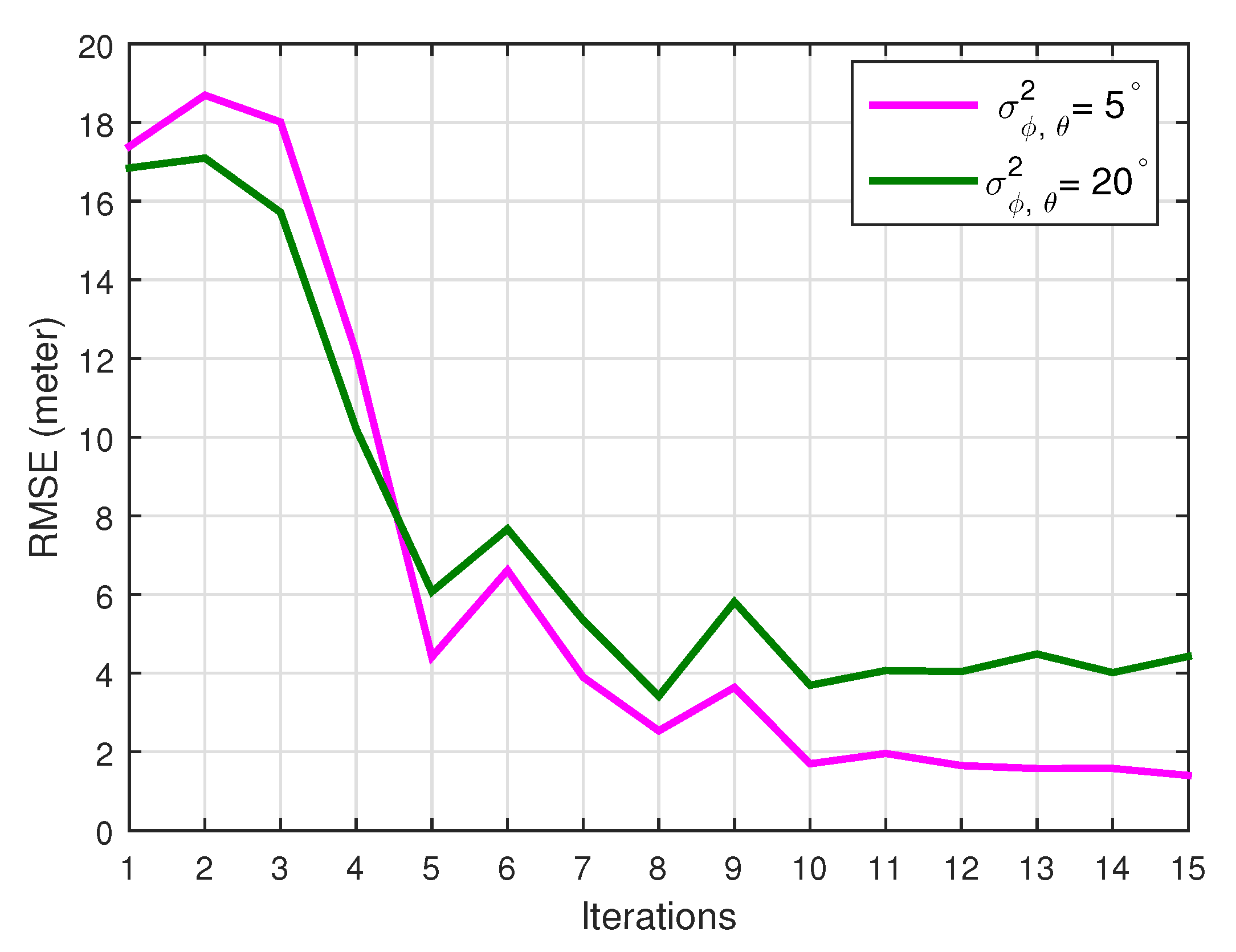
Figure 6, the tracking errors in terms of RMSEs can be much reduced only after five FG iterations. The performances will be further improved and stable with 10 iterations. Moreover, even the standard deviations of the AOA measurement are different, and the convergence behavior is found to be very similar.
6.3. Robustness Analysis
In this subsection, the robustness of tracking performance is evaluated, which is also regarded as the main advantage of the proposed technique. First of all, the effect of sudden sensing errors is considered, such as the false alarm, which may cause unreasonable measurement AOAs. In contrast to the previous simulations, four sensors are used with their positions at , , , and . The reason why more sensors are utilized is to avoid the case in which not enough sensors can work normally when some suffer from significant sensing errors. The FG iteration number is fixed at 15, while 100 snapshots are assumed for measurement at each time index. The real path of the target is set the same as in the previous simulations.
Specifically, at each time index, one of the four sensors is assumed to encounter sudden errors with a probability equal to 0.2, besides the true AOA measurement. Without the help of SI, the fusion center can simply discard the data of a sensor if AOAs from more than one origin are detected. However, the system performance will also decrease when fewer sensors are used. In the proposed system, a predicted AOA will be calculated for each sensor by the fusion center, based on the predicted sensor location by EKF. If the measured AOA is close to the predicted one within a predefined threshold, set by in the simulation, it will be used for location detection at the current time index. Otherwise, the measured data will be discarded. By doing this, sudden errors such as false alarms can be eliminated while still keeping the desired measurement, in order to achieve a better tracking performance.
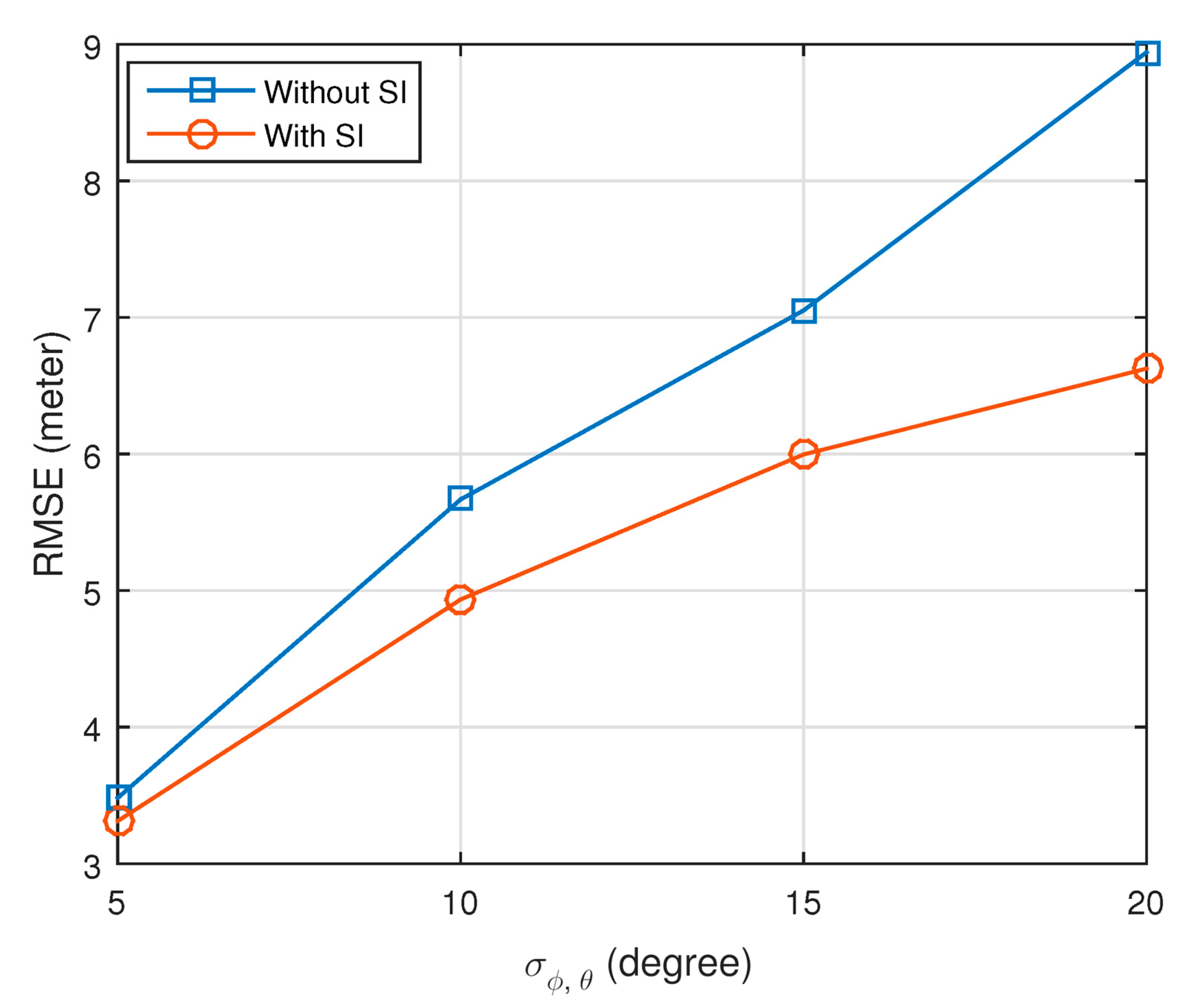
The performance improvement with SI is shown in
Figure 7. Actually, SI is regarded as the a priori information generated from ACRB, which helps the fusion center make a pre-decision to eliminate the impacts of burst sensing errors. In other words, ACRB enables the prediction of the expected AOA measurements. For example, in this simulation of false alarms, if the measured mean AOAs are larger than the predicted values beyond a threshold, i.e.,
, they will be directly eliminated. It can be seen that the RMSEs achieved with SI are always smaller than the cases without SI. The improvement is found to be more significant when the standard deviation of the AOAs becomes larger.
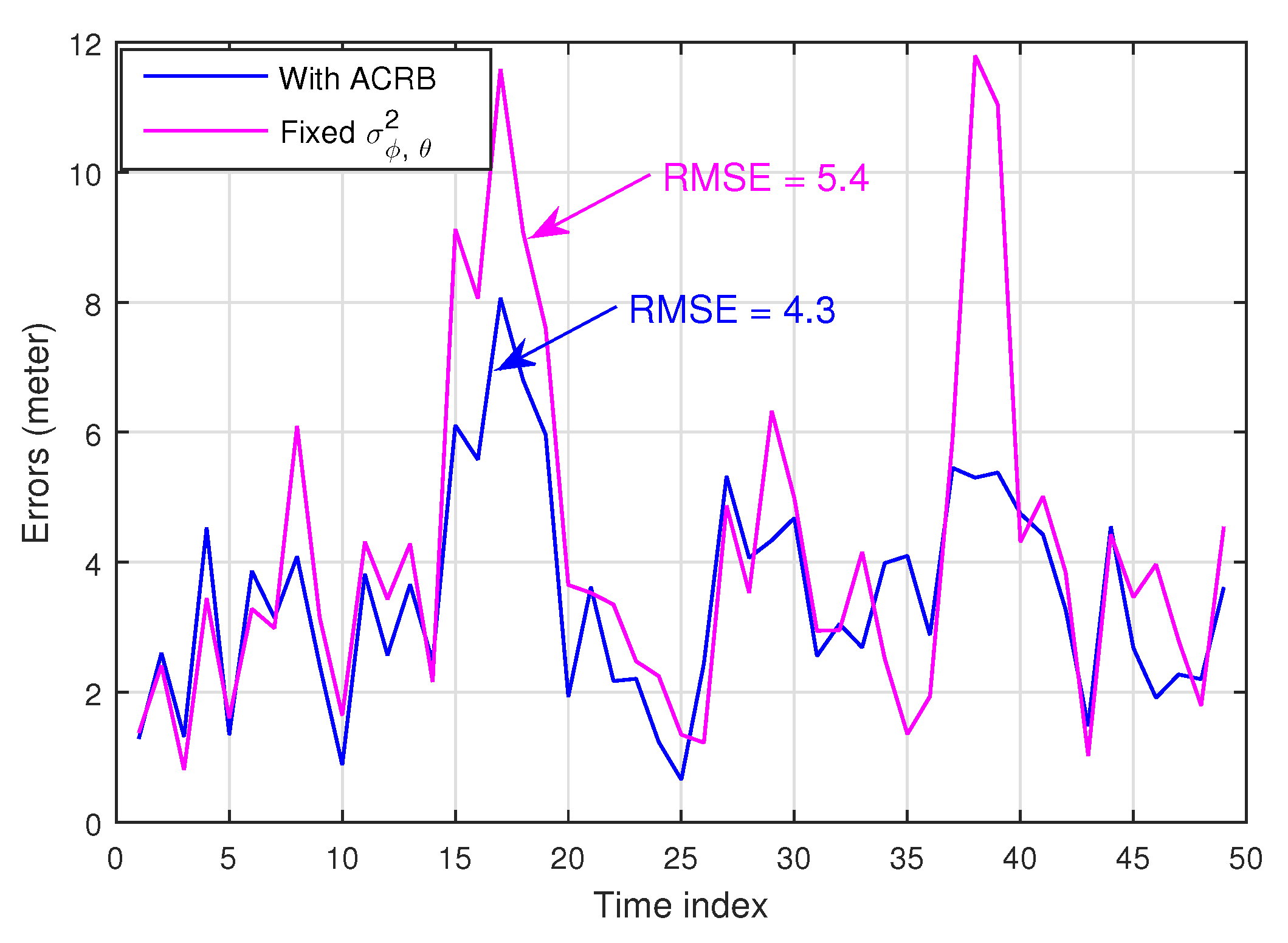
Moreover, simulations are conducted to evaluate the robustness of the system against the dynamic measurement variances. In this case,
is assumed to be randomly chosen from a set of
, for each time index. After location detection, the observation variance is calculated based on the proposed ACRB, which is dynamically fed to the EKF. As a comparative study, another scheme assuming a fixed
equal to two is also simulated. According to
Figure 8, the RMSE achieved by the proposed technique is 4.3, which is smaller than the comparative scheme with the RMSE being 5.4. Obviously, the two local maximum RMSEs appeared for the comparative scheme happen when
was chosen. However, such errors are much reduced with the proposed technique. Therefore, the robustness of the proposed system is proven.
