Analysis of Heat and Mass Transfer for Second-Order Slip Flow on a Thin Needle Using a Two-Phase Nanofluid Model

Abstract

The present paper concentrates on the second-order slip flow over a moving thin needle in a nanofluid. The combined effects of thermophoresis and Brownian motion are considered to describe the heat and mass transfer performance of nanofluid. The resulting system of equations are obtained using similarity transformations and being executed in MATLAB software via bvp4c solver. The physical characteristics of embedded parameters on velocity, temperature, concentration, coefficient of skin friction, heat and mass transfer rates are demonstrated through a graphical approach and are discussed in detail. The obtained outcomes are validated with the existing works and are found to be in good agreement. It is shown that, for a specific domain of moving parameter, dual solutions are likely to exist. The stability analysis is performed to identify the stability of the solutions gained, and it is revealed that only one of them is numerically stable. The analysis indicated that the percentage of increment in the heat and mass transfer rates from no-slip to slip condition for both thin and thick surfaces of the needle ($a=0.1$ and $a=0.2$) are $10.77\%$ and $12.56\%$, respectively. Moreover, the symmetric behavior is noted for the graphs of reduced heat and mass transfer when the parameters $Nb$ and $Nt$ are the same.

1. Introduction

In the world of advanced technology, nanotechnology plays a significant role considering engineering or industrial revolutions in the future, especially for heating and cooling processes. The increment in the heat transfer rate is important as it may reduce the working time as well as lengthen the lifetime of a piece of equipment. Over two decades ago, several methods were developed to improve the heat transfer efficiency rate for working fluids (engine oil, water and ethylene glycol). An attractive method to overcome this limitation by mixing the nanometer-sized (10–50 nm) solid particles called nanoparticles into the working or base fluids was found by Choi [1]. This mixture is regularly known as nanofluids. Interestingly, since nanoparticles have higher thermal conductivity than the base fluids, it is possible to increase the thermal conductivity of the mixture. There are several types of nanomaterials, for instance, carbon nanotubes, metals, composite particles and also carbides. The interesting features of nanomaterials, such as it flows smoothly without blocking the system, have good thermal and physical properties and also the excellence in suspension stability make them much better than the base fluids. In industrial applications, nanoparticles act as a coolant substance to the heat transfer in order to reduce the overheating of instruments. Nanofluids have several applications in transportation, microelectronics, aerospace, medical industries and chemical engineering [2,3,4].

Nanofluid consists of two models namely Buongiorno [5] and Tiwari and Das [6]. The Buongiorno model is a two-phase model that takes into account the effect of thermophoresis and Brownian motion. Meanwhile, Tiwari and Das is a one-phase model that considers the effect of solid nanoparticle volume fractions. The works of Buongiorno have been revised by Nield and Kuznetsov [7] and Kuznetsov and Nield [8] by considering the new boundary condition that has the terms Brownian motion and thermophoresis in the energy and concentration equations [9]. This proposed model is known as a revised model. The first work of nanofluid on the boundary layer flow was done by Khan and Pop [10] by using a stretchable flat surface. Later on, the stagnation point flow on permeable stretching or shrinking sheet in a copper-water nanofluid was studied by Bachok et al. [11]. Observe that in their work, the liquids having nanomaterials obviously enhanced their thermal conductivity and the existence of dual solutions for the shrinking case. The study of the nanofluid flow and heat transfer towards a shrinking surface under the influence of suction is examined by Rohni et al. [12]. A year later, the analysis of heat transfer enhancement of water/functionalized multi-walled carbon nanotube (FMWCNT) past a forward-facing contracting channel was performed by Safaei et al. [13]. The problem of mixed convection flow in a nanofluid was investigated by Goodarzi et al. [14] in a shallow cavity utilizing a two-phase mixture model. Next, the magnetohydrodynamics (MHD) flow under the influence of suction or injection in a nanofluid past a stretching or shrinking surface was analyzed by Naramgari and Sulochana [15]. Since then, tremendous work on nanofluids with different physical situations can be found in references [16,17,18,19,20].

Apart from the commonly used surfaces like stretching or shrinking surface, flat plate or cylinder, there is another surface that plays an important role in the boundary layer flow namely thin or slender needle. The consideration of the thin needle be a major focus since the presence of it in the flow had perturbed the external flow. This flow feature is being observed in the experimental works in order to calculate the velocity and temperature distributions of the system [21]. The utilization of the thin needle is very widespread in industrial and technological purposes, for instance in transportation, coating of wires, blood circulation, geothermal power generation and a hot wire anemometer for computing wind velocity. Notice that, the force convection heat transfer with various surface temperatures in nanofluid using a thin needle has been investigated primarily by Grosan and Pop [22]. Extension to that, the nanofluid flow with variable surface heat flux due to a slender needle near a stagnation point has been examined by Hayat et al. [23]. The study of the Buongiorno mathematical model of nanofluid due to a moving thin needle has been considered by Ahmad et al. [24]. Later on, a numerical computation on the boundary layer flow of a nanofluid by considering prescribed surface heat flux with the stability analysis has been performed by Waini et al. [25]. Just recently, several published works by Salleh et al. [26,27] on a thin needle have been reported for several flow situations.

In recent years, a large number of slip flow models are proposed to illustrate the slip phenomenon occurring at the solid boundaries. Previously, it has been proven that the presumption of flow that adheres no-slip condition on the boundary is no longer appropriate in certain situations, namely rarefied gas flows in micro-scale tools and some coated surfaces. It is necessary to be changed by a partial slip condition especially in cases of suspensions, emulsions, polymer solutions and foams [28]. There are several types of slip models which are 1st order (Maxwell slip model), 2nd order and 1.5 order. The Maxwell [29] slip model is widely applied in current rarefied gas flow. Nevertheless, this model is only applicable to the gas flows in which the rarefaction and roughness effects are not evident. Later on, a classical second-order slip boundary condition is proposed by Beskok and Karniadakis [30]. In their work, they used the model to solve the Navier-Stokes equations for confined fluids at the microscale and nanoscale. Nine years later, the new and advanced second-order slip velocity model has been introduced by Wu [31]. Wu model is an improved slip model from kinetic theory, and it does not suffer from the pressure singularity of the Fukui–Kaneko (FK) model at contact. This model has predictions very close to the numerical solutions of the linearized Boltzmann equation in the whole Knudsen number range. In contrast to other slip models, this model is preferable because it incorporates more in-depth consideration of interaction physics between gas molecules and walls. It is worth knowing that the Wu model has been widely used by many researchers in different flow configurations. For instance, Fang et al. [32] used the model to obtain exact solutions for the governing Navier-Stokes equations by investigating the impact of second-order slip on a viscous flow near a shrinking surface. It is observed that the velocity and wall shear stress are strongly affected by the slip parameters. Nandeppanavar et al. [33] performed the analysis of slip flow and heat transfer with non-linear Navier boundary condition using a stretchable surface. Besides, the study of a magnetic field, second-order slip and thermal radiation effects on nanofluid flow have been done by Hakeem et al. [34] using a stretching or shrinking sheet. The boundary layer flow of a nanofluid with the influences of nanomaterial migration and second-order slip has been examined by Zhu et al. [35]. The latest published works on this topic can be found in references [36,37,38,39].

Note that, there is no published work related to the slip effect with forced convection flow over a continuously moving thin needle using Buongiorno nanofluid model since the works proposed by Ahmad et al. [24] and Salleh et al. [26] few years ago. Thus, the novelty of the present work is to study the effect of the slip in a two-phase nanofluid flow. The applications that is characterized by slip flow at the wall can be found in micro/nano systems such as micropumps, micro-valves, micro-nozzles and hard disk drive. That is by using the similarity transformations, partial differential equations (PDEs) are converted into ordinary differential equations (ODEs) and then are solved numerically via bvp4c solver in MATLAB software (Matlab R2018a, Mathwork, Natick, MA, USA, 1984). The influence of the physical parameters such as first-order slip ($\sigma$), second-order slip ($\delta$), needle thickness (a), velocity ratio or moving parameter ($\epsilon$), Brownian motion ($Nb$) and thermophoresis ($Nt$) on the flow, heat and mass transfer characteristics are presented through figures and tables. Remark that the present work does not only discuss on the physical features of the flow but also discuss on the emergence of multiple solutions along with their stability.

2. Methodology

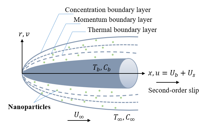
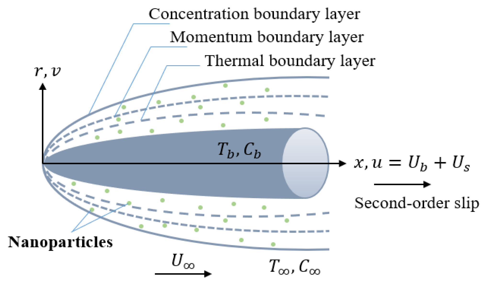
2.1. Governing Equations

In this work, the steady forced convection flow of a nanofluid passing through a moving thin needle with uniform velocity $U_b$ in the same or opposite direction to the free stream $U_{\infty }$ is examined. $U=U_b+U_{\infty }$ is assumed as the composite velocity between the needle and free stream. The system is presumed to be affected by slip. The schematic view of the flow is given in Figure 1 where components u and v are the flow velocities in the direction of x- and r-axis, respectively. Let the needle radius be denoted by $R\left(x\right)$ such that $R\left(x\right)=r={(\nu ax/U)}^{1/2}$. Besides, the surface of the needle is maintained at uniform temperature and concentration, $T_b$ and $C_b$, respectively, and these values are assumed to be greater than the ambient temperature and concentration, $T_{\infty }$ and $C_{\infty }$. The equations that describe the motion, thermal energy and nanoparticle concentration may be written in usual notation as [5,24]:

$$\frac{\partial }{\partial x}\left(ru\right)+\frac{\partial }{\partial r}\left(rv\right)=0,$$

(1)

$$u\frac{\partial u}{\partial x}+v\frac{\partial u}{\partial r}=\frac{\nu }{r}\frac{\partial }{\partial r}\left(r\frac{\partial u}{\partial r}\right),$$

(2)

$$u\frac{\partial T}{\partial x}+v\frac{\partial T}{\partial r}=\frac{\alpha }{r}\frac{\partial }{\partial r}\left(r\frac{\partial T}{\partial r}\right)+\kappa \left[D_B\frac{\partial T}{\partial r}\frac{\partial C}{\partial r}+\frac{D_T}{T_{\infty }}{\left(\frac{\partial T}{\partial r}\right)}^2\right],$$

(3)

$$u\frac{\partial C}{\partial x}+v\frac{\partial C}{\partial r}=\frac{D_B}{r}\frac{\partial }{\partial r}\left(r\frac{\partial C}{\partial r}\right)+\frac{D_T}{T_{\infty }}\frac{1}{r}\frac{\partial }{\partial r}\left(r\frac{\partial T}{\partial r}\right).$$

(4)

The relevant boundary conditions for the above equations are:

$$u=U_b+U_s,v=0,T=T_b,D_B\frac{\partial C}{\partial r}+\frac{D_T}{T_{\infty }}\frac{\partial T}{\partial r}=0\mathrm{at}r=R\left(x\right),$$

$$u\to U_{\infty },T\to T_{\infty },C\to C_{\infty }\mathrm{as}r\to \infty ,$$

(5)

where $\nu$ is the kinematic viscosity, $\alpha$ is the thermal diffusivity, $\kappa ={\left(\rho C_p\right)}_s/{\left(\rho C_p\right)}_f$ is the ratio of nanofluid effective heat capacity where terms ‘s’ and ‘f’ denoted solid nanomaterial and base fluid, T and C are the temperature and concentration of nanofluid, respectively, $D_B$ is the Brownian diffusion coefficient, $D_T$ is the thermophoretic diffusion coefficient and $U_s$ is the slip velocity at the needle. Following Wu’s model, the slip velocity is given as:

$$U_s=\frac{2}{3}\left(\frac{3-\omega h^3}{\omega }-\frac{3}{2}\frac{1-h^2}{K_n}\right)\zeta \frac{\partial u}{\partial r}-\frac{1}{4}\left[h^4+\frac{2}{K_n^2}(1-h^2)\right]{\zeta }^2\frac{{\partial }^{2}u}{\partial r^2}=A_1\frac{\partial u}{\partial r}+A_2\frac{{\partial }^{2}u}{\partial r^2},$$

(6)

where $h=\min (1/K_n,1)$, $K_n$ is the Knudsen number, $\omega$ is the momentum accommodation coefficient such that $0\le \omega \le 1$, $\zeta$ is the molecular mean free path, $A_1=L_{1}x/r$ and $A_2=L_{2}x$ are first and second-order slip coefficients, and $L_1$ and $L_2$ denoted their respective slip lengths. Follow the definition of h, one may observed that for any given value of $K_n$, the value of h is limited to a certain range of $0\le h\le 1$. Since $\zeta$ is always positive, hence, the constant parameter $A_2$ will take the negative value.

Next, the following similarity transformations are introduced to convert the PDEs (2)–(5) into dimensionless form [5,7,8]:

$$\psi (x,r)=\nu xf\left(\eta \right),\eta =\frac{U{r}^2}{\nu x},\theta \left(\eta \right)=\frac{T-T_{\infty }}{T_b-T_{\infty }},\varphi \left(\eta \right)=\frac{C-C_{\infty }}{C_{\infty }}.$$

(7)

Here $\psi (x,r)$ is the stream function such that $u=r^{-1}\partial \psi /\partial r$ and $v=-r^{-1}\partial \psi /\partial x$. In Equation (7), $\theta \left(\eta \right)$ and $\varphi \left(\eta \right)$ are the dimensionless temperature and concentration and $\eta$ is the similarity variable.

Using the similarity transformations (7), Equations (2)–(4) along with (5) can be written as:

$$2\left(\eta f^{‴}+f^{″}\right)+f{f}^{″}=0,$$

(8)

$$\frac{2}{\mathrm{Pr}}(\eta {\theta }^{″}+{\theta }^{\prime })+2\eta \left(Nt{{\theta }^{\prime }}^2+Nb{\theta }^{\prime }{\varphi }^{\prime }\right)+f{\theta }^{\prime }=0,$$

(9)

$$2(\eta {\varphi }^{″}+{\varphi }^{\prime })+2\frac{Nt}{Nb}(\eta {\theta }^{″}+{\theta }^{\prime })+\mathrm{Le}f{\varphi }^{\prime }=0,$$

(10)

where Equation (1) is satisfied identically and the transformed boundary conditions are:

$$f\left(a\right)=\frac{\epsilon }{2}a+(\sigma +\delta )a{f}^{″}\left(a\right)+2\delta a^2{f}^{‴}\left(a\right),f^{\prime }\left(a\right)=\frac{\epsilon }{2}+(\sigma +\delta )f^{″}\left(a\right)+2\delta a{f}^{‴}\left(a\right),\theta \left(a\right)=1,$$

$$Nb{\varphi }^{\prime }\left(a\right)+Nt{\theta }^{\prime }\left(a\right)=0,$$

$$f^{\prime }\left(\eta \right)\to \frac{1-\epsilon }{2},\theta \left(\eta \right)\to 0,\varphi \left(\eta \right)\to 0\mathrm{as}\eta \to \infty .$$

(11)

Here prime indicated the differentiation with respect to $\eta$, $\mathrm{Pr}=\nu /\alpha$ is the Prandtl number, $Nt=D_T\kappa (T_b-T_{\infty })/\nu T_{\infty }$ is the thermophoresis parameter, $Nb=D_B\kappa (C_b-C_{\infty })/\nu$ is the Brownian movement parameter, $\mathrm{Le}=\nu /D_B$ is the Lewis number and $\epsilon =U_b/U$ is the velocity ratio parameter with $\epsilon <0$ represented the needle against the free stream, whilst $\epsilon >0$ represented the needle is in the same direction as the free stream. In boundary conditions (11), a is the needle thickness by assuming $\eta =a$, $\sigma =2U{L}_1/\nu$ is the first-order slip parameter with $\sigma >0$ and $\delta =2U{L}_2/\nu$ denoted the second-order slip parameter with $\delta <0$.

The expressions of the skin friction coefficients $C_f$, local Nusselt number $N{u}_x$ and local Sherwood number $S{h}_x$, respectively, are:

$$C_f=\frac{\mu }{\rho U^2}{\left(\frac{\partial u}{\partial r}\right)}_{r=a}=4R{e}_x^{-1/2}{a}^{1/2}{f}^{″}\left(a\right),$$

(12)

$$N{u}_x=\frac{x}{(T_b-T_{\infty })}{\left(\frac{\partial T}{\partial r}\right)}_{r=a}=-2R{e}_x^{1/2}{a}^{1/2}{\theta }^{\prime }\left(a\right),$$

(13)

$$S{h}_x=\frac{-x}{C_{\infty }}{\left(\frac{\partial C}{\partial r}\right)}_{r=a}=-2R{e}_x^{1/2}{a}^{1/2}{\varphi }^{\prime }\left(a\right),$$

(14)

in which $R{e}_x=Ux/\nu$ is the local Reynolds number.

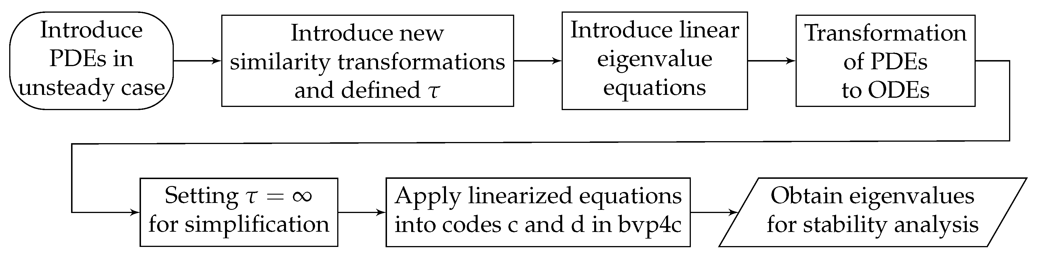
2.2. Stability Analysis

In the present study, it is noticed that there exist the solution branches against a single parameter. In this case, it is essential to find out the physical credibility of the solutions obtained. The outputs obtained from the stability analysis could be applied in engineering applications. Regarding this, the stability of solutions is conducted here. To perform this analysis, Equations (2)–(5) must be introduced in unsteady-state by initiating the dimensionless time variable $\tau =2Ut/x$, thus, obtain the followings (see Merkin [40] and Weidman et al. [41]):

$$\frac{\partial u}{\partial t}+u\frac{\partial u}{\partial x}+v\frac{\partial u}{\partial r}=\frac{\nu }{r}\frac{\partial }{\partial r}\left(r\frac{\partial u}{\partial r}\right),$$

(15)

$$\frac{\partial T}{\partial t}+u\frac{\partial T}{\partial x}+v\frac{\partial T}{\partial r}=\frac{\alpha }{r}\frac{\partial }{\partial r}\left(r\frac{\partial T}{\partial r}\right)+\kappa \left[D_B\frac{\partial T}{\partial r}\frac{\partial C}{\partial r}+\frac{D_T}{T_{\infty }}{\left(\frac{\partial T}{\partial r}\right)}^2\right],$$

(16)

$$\frac{\partial C}{\partial t}+u\frac{\partial C}{\partial x}+v\frac{\partial C}{\partial r}=\frac{D_B}{r}\frac{\partial }{\partial r}\left(r\frac{\partial C}{\partial r}\right)+\frac{D_T}{T_{\infty }}\frac{1}{r}\frac{\partial }{\partial r}\left(r\frac{\partial T}{\partial r}\right).$$

(17)

The new look of similarity transformations are as follows:

$$\psi =\nu xf(\eta ,\tau ),\eta =\frac{U{r}^2}{\nu x},\theta (\eta ,\tau )=\frac{T-T_{\infty }}{T_b-T_{\infty }},\varphi (\eta ,\tau )=\frac{C-C_{\infty }}{C_{\infty }},\tau =\frac{2Ut}{x}.$$

(18)

Due to Equation (18), Equations (15)–(17) can be expressed as:

$$2\left(\eta \frac{{\partial }^{3}f}{\partial {\eta }^3}+\frac{{\partial }^{2}f}{\partial {\eta }^2}\right)+f\frac{{\partial }^{2}f}{\partial {\eta }^2}+\tau \frac{\partial f}{\partial \eta }\frac{{\partial }^{2}f}{\partial \eta \partial \tau }-\tau \frac{{\partial }^{2}f}{\partial {\eta }^2}\frac{\partial f}{\partial \tau }-\frac{{\partial }^{2}f}{\partial \eta \partial \tau }=0,$$

(19)

$$\frac{2}{\mathrm{Pr}}\left(\eta \frac{{\partial }^2\theta }{\partial {\eta }^2}+\frac{\partial \theta }{\partial \eta }\right)+f\frac{\partial \theta }{\partial \eta }+2\eta \left(Nb\frac{\partial \theta }{\partial \eta }\frac{\partial \varphi }{\partial \eta }+Nt\frac{\partial \theta }{\partial \eta }\frac{\partial \theta }{\partial \eta }\right)-\frac{\partial \theta }{\partial \tau }+\tau \frac{\partial f}{\partial \eta }\frac{\partial \theta }{\partial \tau }-\tau \frac{\partial f}{\partial \tau }\frac{\partial \theta }{\partial \eta }=0,$$

(20)

$$2\left(\eta \frac{{\partial }^2\varphi }{\partial {\eta }^2}+\frac{\partial \varphi }{\partial \eta }\right)+2\frac{Nt}{Nb}\left(\eta \frac{{\partial }^2\theta }{\partial {\eta }^2}+\frac{\partial \theta }{\partial \eta }\right)+\mathrm{Le}f\frac{\partial \varphi }{\partial \eta }-\mathrm{Le}\frac{\partial \varphi }{\partial \tau }+\tau \mathrm{Le}\frac{\partial f}{\partial \eta }\frac{\partial \varphi }{\partial \tau }-\tau \mathrm{Le}\frac{\partial f}{\partial \tau }\frac{\partial \varphi }{\partial \eta }=0,$$

(21)

and boundary conditions are reframed as:

$$f(a,\tau )=\frac{\epsilon }{2}a+(\sigma +\delta )a\frac{{\partial }^{2}f}{\partial {\eta }^2}(a,\tau )+2\delta a^2\frac{{\partial }^{3}f}{\partial {\eta }^3}(a,\tau )+\tau \frac{\partial f}{\partial \tau }(a,\tau ),\theta (a,\tau )=1,$$

$$\frac{\partial f}{\partial \eta }(a,\tau )=\frac{\epsilon }{2}+(\sigma +\delta )\frac{{\partial }^{2}f}{\partial {\eta }^2}(a,\tau )+2\delta a\frac{{\partial }^{3}f}{\partial {\eta }^3}(a,\tau ),Nb\frac{\partial \varphi }{\partial \eta }(a,\tau )+Nt\frac{\partial \theta }{\partial \eta }(a,\tau )=0,$$

$$\frac{\partial f}{\partial \eta }(\eta ,\tau )\to \frac{1}{2}(1-\epsilon ),\theta (\eta ,\tau )\to 0,\varphi (\eta ,\tau )\to 0\mathrm{as}\eta \to \infty .$$

(22)

Now linear eigenvalue equations are introduced as follows [41]:

$$f(\eta ,\tau )=f_0\left(\eta \right)+e^{-\xi \tau }F(\eta ,\tau ),\theta (\eta ,\tau )={\theta }_0\left(\eta \right)+e^{-\xi \tau }G(\eta ,\tau ),\varphi (\eta ,\tau )={\varphi }_0\left(\eta \right)+e^{-\xi \tau }H(\eta ,\tau ),$$

(23)

to examine the stability of solutions $f=f_0\left(\eta \right)$, $\theta ={\theta }_0\left(\eta \right)$ and $\varphi ={\varphi }_0\left(\eta \right)$ which satisfied the boundary value problem in Equations (19)–(22). The small relative to $f_0\left(\eta \right)$, ${\theta }_0\left(\eta \right)$ and ${\varphi }_0\left(\eta \right)$, respectively are given as $F(\eta ,\tau )$, $G(\eta ,\tau )$ and $H(\eta ,\tau )$ and $\xi$ denoted the eigenvalue.

After using Equation (23), Equations (19)–(22) are changed to:

$$2\left(\eta F_0^{‴}+F_0^{″}\right)+f_0{F}_0^{″}+f_0^{\prime \prime }{F}_0+\xi F_0^{\prime }=0,$$

(24)

$$\frac{2}{\mathrm{Pr}}\left(\eta G_0^{″}+G_0^{\prime }\right)+f_0{G}_0^{\prime }+F_0{\theta }_0^{\prime }+2\eta Nb\left({\theta }_0^{\prime }{H}_0^{\prime }+{\varphi }_0^{\prime }{G}_0^{\prime }\right)+4\eta Nt{\theta }_0^{\prime }{G}_0^{\prime }+\xi G_0=0,$$

(25)

$$2\left(\eta H_0^{″}+H_0^{\prime }\right)+2\frac{Nt}{Nb}\left(\eta G_0^{″}+G_0^{\prime }\right)+\mathrm{Le}{f}_0{H}_0^{\prime }+Le{F}_0{\varphi }_0^{\prime }+\xi \mathrm{Le}{H}_0=0,$$

(26)

and the boundary conditions are:

$$F_0\left(a\right)=(\sigma +\delta )a{F}_0^{″}\left(a\right)+2\delta a^2{F}_0^{‴}\left(a\right),F_0^{\prime }\left(a\right)=(\sigma +\delta )F_0^{″}\left(a\right)+2\delta a{F}_0^{‴}\left(a\right),$$

$$G_0\left(a\right)=0,Nb{H}_0^{\prime }\left(a\right)+Nt{G}_0^{\prime }\left(a\right)=0,$$

$$F_0^{\prime }\left(\eta \right)\to 0,G_0\left(\eta \right)\to 0,H_0\left(\eta \right)\to 0\mathrm{as}\eta \to \infty .$$

(27)

To find the eigenvalue, $\tau$ must be assumed as zero indicating an initial decay or growth of the solution (23). Hence, functions $F(\eta ,\tau )$, $G(\eta ,\tau )$ and $H(\eta ,\tau )$ can be written as $F_0\left(\eta \right)$, $G_0\left(\eta \right)$ and $H_0\left(\eta \right)$, respectively. Based on the previous published paper by Harris et al. [42], the boundary conditions can be relaxed either on $F_0^{\prime }\left(\eta \right)$, $G_0\left(\eta \right)$ or $H_0\left(\eta \right)$ to determine the possible minimum eigenvalue. In this work, the condition $F_0^{\prime }\left(\eta \right)\to 0$ as $\eta \to \infty$ is selected to be relaxed, thus, Equations (24)–(27) are computed along with the new condition $F_0^{″}\left(a\right)=1$.

2.3. Numerical Approach

The nonlinear differential Equations (8)–(10) subject to the conditions (11) are executed through bvp4c solver in MATLAB software. In this solver, the initial guess at the starting mesh point is identified and the step size is changed to obtain the appropriate precisions. Despite that, it is compulsory to convert the differential equations into the first-order system of equation. Thus, the suitable variables used to reduce the equations have been introduced as follows:

$$f\left(\eta \right)=y_1,f^{\prime }\left(\eta \right)=y_2,f^{″}\left(\eta \right)=y_3,\theta \left(\eta \right)=y_4,{\theta }^{\prime }\left(\eta \right)=y_5,\varphi \left(\eta \right)=y_6,{\varphi }^{\prime }\left(\eta \right)=y_7.$$

(28)

Therefore, Equations (8)–(10) are reframed as:

$$f^{‴}\to y_3^{\prime }=-\frac{1}{\eta }\left(y_3+\frac{1}{2}{y}_1{y}_3\right),$$

(29)

$${\theta }^{″}\to y_5^{\prime }=-\frac{1}{\eta }\left(y_5+\frac{\mathrm{Pr}}{2}{y}_1{y}_5+\mathrm{Pr}\eta Nb{y}_5{y}_7+\mathrm{Pr}\eta Nt{y}_5{y}_5\right),$$

(30)

$${\varphi }^{″}\to y_7^{\prime }=-\frac{1}{\eta }\left(y_7+\eta \frac{Nt}{Nb}{y}_5^{\prime }+\frac{Nt}{Nb}{y}_5+\frac{\mathrm{Le}}{2}{y}_1{y}_7\right),$$

(31)

with the boundary conditions:

$$y_1\left(c\right)=\frac{\epsilon }{2}a+(\sigma +\delta )a{y}_3\left(c\right)+2\delta a^2{y}_3^{\prime }\left(c\right),y_2\left(c\right)=\frac{\epsilon }{2}+(\sigma +\delta )y_3\left(c\right)+2\delta a{y}_3^{\prime }\left(c\right),$$

$$y_4\left(c\right)=1,Nb{y}_7\left(c\right)+Nt{y}_5\left(c\right)=0,$$

$$y_2\left(d\right)\to \frac{1}{2}(1-\epsilon ),y_4\left(d\right)\to 0,y_6\left(d\right)\to 0\mathrm{as}\eta \to \infty ,$$

(32)

where c and d are the situations at the needle wall ($\eta =a$) and free stream ($\eta ={\eta }_{\infty }$), respectively. In this work, all the physical parameters are varied throughout the entire paper. The numerical results are obtained by estimating the inputs of unfixed parameters which satisfied the condition $f^{\prime }\left(\eta \right)\to (1-\epsilon )/2$, $\theta \left(\eta \right)\to 0$ and $\varphi \left(\eta \right)\to 0$ as $\eta \to \infty$. The procedure must be reiterated until the converged output meets a tolerance limit of ${10}^{-6}$.

Considering the same procedures as discussed above, the solution for the stability analysis can also be computed using Equations (24)–(26) along with the conditions (27). The obtained results indicated the solutions are stable if eigenvalue took the positive value, whilst the solutions are unstable if there exists a negative sign at the eigenvalue. Throughout this study, the suitable values of $\eta$ are taken from 10 up to ${\eta }_{\infty }=60$, in which ${\eta }_{\infty }$ situated outside the boundary layer thicknesses.

It is worth mentioning that there are four major codes involved in the bvp4c solver. The first code, also known as the initial guess code (code a), is used to find the initial guess for the upper and lower branch solutions. In this regard, two sets of initial guesses are required to estimate the initial solutions for both upper and lower branch solutions. Second is the continuation code (code b) where the same ODEs and boundary conditions as in the first code are applied to compute the numerical solution of the problem. The function of this code is to find the other solutions which are near to the initial guess in the first code. Meanwhile, the third code (upper solution code or code c) and the fourth code (lower solution code or code d) are used to determine the minimum eigenvalues $\xi$ for upper and lower branch solutions, respectively.

The summary of the steps for solving this problem is shown in Figure 2 and Figure 3 for both numerical solutions and eigenvalues.

2.4. Code of Verification

In order to validate the accuracy of the developed numerical scheme, the obtained results of reduced skin friction $f^{″}\left(a\right)$ have been verified with those discussed by Ahmad et al. [24]. In this comparison, the multiple values of needle thickness a are considered and are found to be in an excellent agreement with the previous study as depicted in

Table 1. Comparison values of $f^{″}\left(a\right)$ when $\sigma =\delta =\epsilon =0$ and $\mathrm{Pr}=1$ for several values of a.

Needle Thickness a	Ahmad et al. [24]	Present Study
0.1	1.2888171	1.2888299
0.01	8.4924360	8.4924452
0.001	62.163672	62.163606

.

3. Results and Discussion

The important features of all physical parameters such as first-order slip parameter $\sigma$, second-order slip parameter $\delta$, needle thickness a, ratio of velocity or moving parameter $\epsilon$, thermophoresis parameter $Nt$ and Brownian motion parameter $Nb$ are highlighted and discussed in this section. The numerical outcomes which consists of wall shear stress $f^{″}\left(a\right)$, reduced heat transfer $-{\theta }^{\prime }\left(a\right)$, reduced mass transfer $-{\varphi }^{\prime }\left(a\right)$, velocity $f^{\prime }\left(\eta \right)$, temperature $\theta \left(\eta \right)$ and concentration $\varphi \left(\eta \right)$ fields, as well as heat transfer rate (or local Nusselt number) ${\left(R{e}_x\right)}^{-1/2}N{u}_x$ and mass transfer rate (or local Sherwood number) ${\left(R{e}_x\right)}^{-1/2}S{h}_x$ are demonstrated in Figure 4, Figure 5, Figure 6 and Figure 7 and

Table 2. Heat and mass transfer rate for some values of $Nt$, $\sigma$, $\delta$ and a when $Nb=0.3$, $\epsilon =-2.4$ and $\mathrm{Pr}=\mathrm{Le}=1$.

$\mathit{N}\mathit{t}$	$\mathbf{\sigma }$	$\mathbf{\delta }$	${\left({\mathit{R}\mathit{e}}_{\mathit{x}}\right)}^{-1/2}{\mathit{N}\mathit{u}}_{\mathit{x}}$		${\left({\mathit{R}\mathit{e}}_{\mathit{x}}\right)}^{-1/2}{\mathit{S}\mathit{h}}_{\mathit{x}}$
			$\mathit{a}=0.1$	$\mathit{a}=0.2$	$\mathit{a}=0.1$	$\mathit{a}=0.2$
0.1	0	0	1.401166	0.866509	0.467055	0.288836
	0.01	−0.02	1.552031	0.975379	0.517344	0.325126
0.2			1.558873	0.987418	1.039248	0.658279
0.3			1.565787	0.999750	1.565787	0.999750
0.4			1.572775	1.012387	2.097033	1.349849
0.1	0.02	−0.03	1.646401	1.046715	0.548800	0.348904
	0.03	−0.04	1.733750	1.115544	0.577916	0.371847
	0.04	−0.05	1.814040	1.182290	0.604680	0.394096

,

Table 3. Mass transfer rate for some values of $Nb$ and $Nt$ when $\sigma =0.02$, $\delta =-0.03$, $\epsilon =-2.4$, $a=0.1$ and $\mathrm{Pr}=\mathrm{Le}=2$.

$\mathit{N}\mathit{b}$	${\left({\mathit{R}\mathit{e}}_{\mathit{x}}\right)}^{-1/2}{\mathit{S}\mathit{h}}_{\mathit{x}}$
	$\mathit{N}\mathit{t}=0.1$	$\mathit{N}\mathit{t}=0.2$	$\mathit{N}\mathit{t}=0.3$	$\mathit{N}\mathit{t}=0.4$	$\mathit{N}\mathit{t}=0.5$
0.1	1.643715	3.333979	5.073028	6.863222	8.707038
0.3	0.547905	1.111326	1.691009	2.287740	2.902346
0.5	0.328743	0.666795	1.014605	1.372644	1.741407

and

Table 4. Minimum eigenvalues for multiple values of $\sigma$, $\delta$ and $\epsilon$.

Slip Parameters	$\mathbf{\epsilon }$	Upper Branch Solutions	Lower Branch Solutions
$\sigma =0.02,\delta =-0.01$	−5.2248	0.0482	−0.0463
	−5.224	0.0503	−0.0483
	−5.22	0.0597	−0.0568
$\sigma =0.03,\delta =-0.02$	−6.0862	0.0256	−0.0251
	−6.086	0.0266	−0.0261
	−6.08	0.0483	−0.0467
$\sigma =0.04,\delta =-0.03$	−7.1624	0.0169	−0.0167
	−7.162	0.0200	−0.0197
	−7.16	0.0312	−0.0306

.

Figure 4a–c are illustrated to present the influence of $\sigma$ on the variation of $f^{″}\left(a\right)$, $-{\theta }^{\prime }\left(a\right)$ and $-{\varphi }^{\prime }\left(a\right)$ with $\epsilon$ when the second-order slip effect is absent ($\delta =0$). It can be seen in Figure 4a,b that when there is no second-order slip, the wall shear stress and thermal energy flux enhance with the increase in the first-order slip parameter. Meanwhile, in Figure 4c the reduction of mass flux is noted for higher values of $\sigma$. In this proposed model, the occurrence of slip decreases the momentum and thermal layer thicknesses and thus, increasing both drag force and thermal energy flux on the needle wall. The fact that the presence of slip in the system slows down the separation of the boundary layer and this phenomenon is proven through turning points ${\epsilon }_c$ that unifies both upper and lower branch solutions. Further, it is seen that as the values of $\sigma$ magnify from $\sigma =0.02$ to $\sigma =0.04$, turning points are observed to diminish from ${\epsilon }_c=-4.9154$ to ${\epsilon }_c=-5.8289$. This implies that the slip parameter gives a significant impact on the emergence of dual solutions. Besides, it is observed from Figure 4b,c that the graph for $-{\varphi }^{\prime }\left(a\right)$ is a reflection of the graph $-{\theta }^{\prime }\left(a\right)$ because of the value of $Nb$ and $Nt$ considered is the same.

Figure 5a–c are plotted to observe the effect of $\sigma$ and $\delta$ on the variation of $f^{″}\left(a\right)$, $-{\theta }^{\prime }\left(a\right)$, and $-{\varphi }^{\prime }\left(a\right)$ with $\epsilon$. It is observed from the plot that by enhancing the values of $\sigma$ and |$\delta$| will accelerate the needle shear stress and thermal energy flux, whilst the opposite behavior is noticed for the mass flux. Different from Figure 4a–c, the region of the solutions obtained is seen to be increased when the second-order slip is imposed. This can be proven by looking at $\sigma =0.04$ in Figure 4a and $\sigma =0.04$ and $\delta =-0.03$ in Figure 5a where the solutions obtained expand from $-5.8289$ to $-7.1634$. Other than that, it is revealed that the turning points ${\epsilon }_c$ decrease as the combined slip parameters ascend. Moreover, the existence of dual solutions are noticed when the needle opposes the free stream direction or when the moving parameter takes the negative value ($\epsilon <0$). Visibly, the dual solutions appear in a specific domain of ${\epsilon }_c<\epsilon \le -1$ and there are unique solutions when $\epsilon >-1$. Remark that this variation is much better compared to the variation that contains only the first-order slip parameter where its magnitude of $f^{″}\left(a\right)$, $-{\theta }^{\prime }\left(a\right)$, and $-{\varphi }^{\prime }\left(a\right)$ is quite higher than the previous one.

The effect of parameters $Nt$, $\sigma$, $\delta$ and a on heat and mass transfer rates are displayed in Table 2. Since parameter $Nt$ does not alter Equation (8), thus numerical solutions are only computed for Equations (9) and (10). As can be seen, the rate of heat and mass transfer from the surface to the fluid increase with the increasing value of $Nt$. Physically, as the values of $Nt$ intensify the force of a temperature gradient known as the thermophoretic force increases as well. This situation will produce larger kinetic energy for suspended molecules and the presence of higher thermophoretic force will push the molecules away from the needle. As a consequence, accelerating heat and mass transfer in the system. Besides, in the case of a thin surface of the needle ($a=0.1$), it is observed that heat and mass transfer rate enhance by $10.77\%$ when the slip effect ($\sigma =0.01$ and $\delta =-0.02$) is considered. Meanwhile, in the case of a thick surface of the needle ($a=0.2$), the percentage of increment in the heat and mass transfer rates is about $12.56\%$. It is also revealed that the higher value of slip parameters leads to a better performance of thermal energy and mass transfer on the surface. This happens due to the reduction in the thermal and concentration boundary layer thicknesses. The reason for this is based on the fact that the slippery surface of the needle complicates the formation of the boundary layer near the surface. Hence, speed up the rate of heat and mass transfer. As expected, the heat and mass transfer rates for a thin surface ($a=0.1$) is higher compared to a thick surface ($a=0.2$). The fact that the thermal energy and mass are easily penetrated into a thin surface rather than a thick one. This is because, inside the thin surface, fewer molecules are in contact with each other.

The mass transfer rates for several values of $Nb$ and $Nt$ are presented in Table 3. It is seen that the greater rate of the Brownian motion decelerates the transportation of mass from the needle to the fluid phase. In the presence of more suspended particles (base fluid particles and nanoparticles) in the flow, the Brownian motion and its kinetic energy cause the liquid to become more viscous and consequently slow down the transmission of mass. This led to a reduction in the mass transfer rate at the surface. Since Equation (9) does not have the term $Nb$ after replacing the condition $Nb{\varphi }^{\prime }\left(a\right)+Nt{\theta }^{\prime }\left(a\right)=0$ inside, hence, the parameter $Nb$ does not give any impact on the temperature gradient and heat transfer rate. Apart from that, the increase in the parameter $Nt$ offers a larger magnitude of mass transfer rate. The explanation of this trend is similar to the previous paragraph.

The variation of $f^{\prime }\left(\eta \right)$, $\theta \left(\eta \right)$ and $\varphi \left(\eta \right)$ for several values of first-order slip parameter, second-order slip parameter and thermophoresis parameter are given in Figure 6a–c and Figure 7a,b. These figures revealed that the obtained profiles have achieved the prerequisites of far field boundary conditions (11) asymptotically. Therefore, it can be confidently said that the numerical results gained from the present work are precise. It is essential to stress that the dual nature of solutions in Figure 4 and Figure 5 has been supported by the existence of dual velocity, temperature and concentration in these figures. As predicted, the boundary layer thickness for the lower branch solution is thicker than the upper branch solution.

The variation of minimum eigenvalue $\xi$ for multiple values of slip parameters ($\sigma$ and $\delta$) and moving parameter $\epsilon$ when $Nb=Nt=0.3$, $\mathrm{Pr}=2$, $\mathrm{Le}=1$ and $a=0.1$ are presented in Table 4. These computational outputs have been executed from the linear eigenvalue Equations (24)–(27) for stability analysis. As can be observed, the upper branch solution has positive minimum eigenvalue which indicated the initial disturbances decay slowly with time. Meanwhile, the opposite trend is noted for the lower branch solution. Thus, it is worth to mention that the solution for the upper branch is numerically stable in all cases.

4. Conclusions

In this paper, the problem of steady laminar forced convection flow past a continuously moving thin needle with slip effect has been investigated. The numerical solutions for momentum, energy and concentration equations were computed by the bvp4c solver in MATLAB software. The summaries of the current analysis are listed as follows.

• The presence of slip increases the surface shear stress, heat and mass transfer rates at the needle surface. It also widens the range of the existing solution.
• The reduction of needle thickness causes more friction to take place on the surface and increases heat and mass transfer rates inside the flow.
• The heat and mass transfer rates enhance with the increasing values of the thermophoresis parameter.
• The mass transfer rate diminishes with higher Brownian motion parameter.
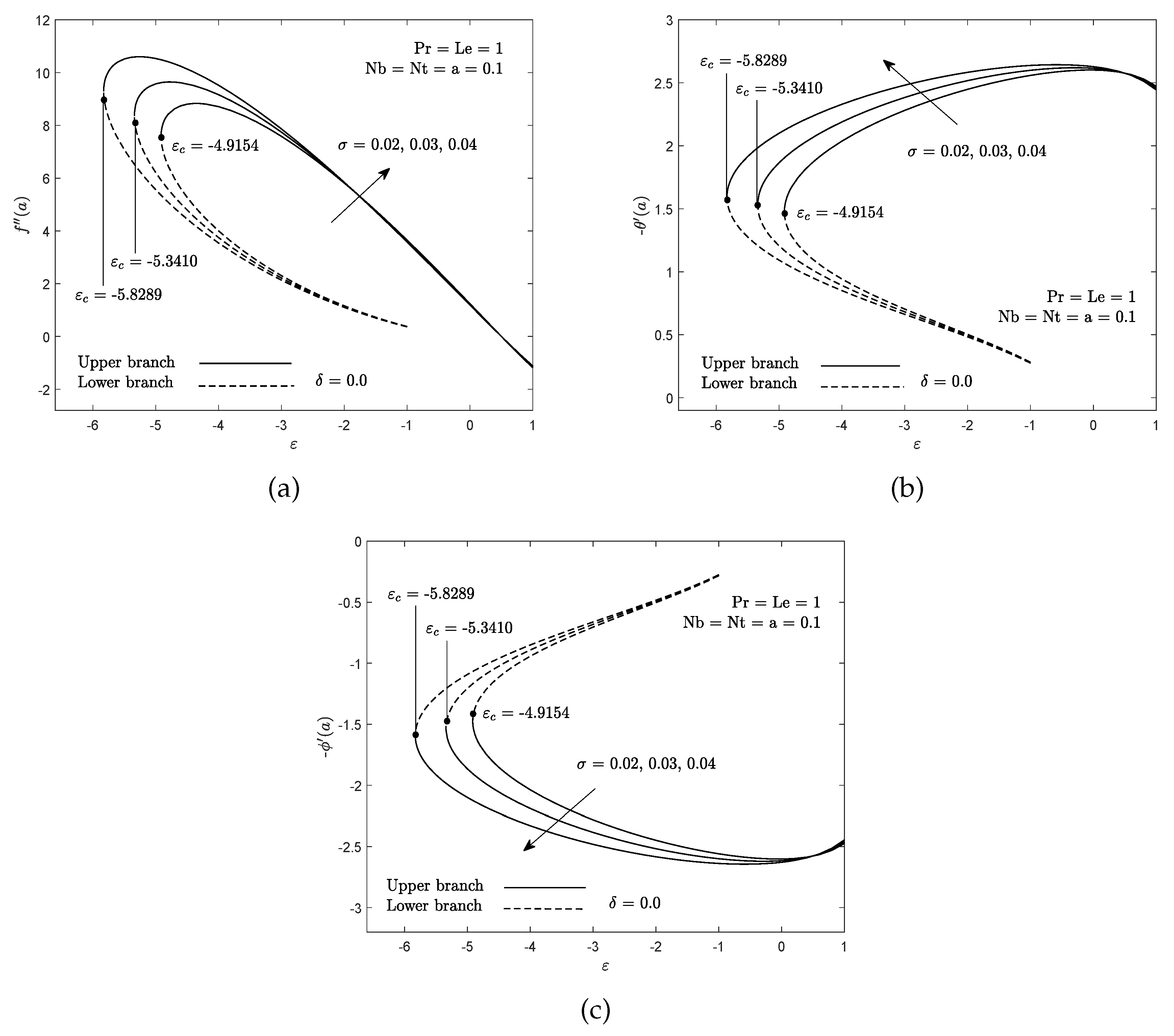
• Multiple solutions arise when the free stream and needle move in the opposite direction.
• The credibility of the upper branch solution has been confirmed using a stability analysis.

5. Future Works

Researchers have not been so concerned with consideration of a thin needle in the boundary layer flow of a two-phase nanofluid. Hence, more studies regarding this matter need to be carried out. The topic of the thin needle is interesting due to the motion of the needle that distracts the free stream direction. By investigating the current problem, it is believed that the proposed work can assist engineers to create certain applications that require high heat and mass transfer rates.

References

1. Choi, S.U.S. Enhancing thermal conductivity of fluids with nanoparticles. Am. Soc. Mech. Eng. Fluids Eng. Div. 1995, 231, 99–105. [Google Scholar]
2. Saidur, R.; Leong, K.Y.; Mohammad, H.A. A review on applications and challenges of nanofluids. Renew. Sustain. Energy Rev. 2011, 15, 1646–1668. [Google Scholar] [CrossRef]
3. Huminic, G.; Huminic, A. Application of nanofluids in heat exchangers: A review. Renew. Sustain. Energy Rev. 2012, 16, 5625–5638. [Google Scholar] [CrossRef]
4. Sajid, M.U.; Ali, H.M. Recent advances in application of nanofluids in heat transfer devices: A critical review. Renew. Sustain. Energy Rev. 2019, 103, 556–592. [Google Scholar] [CrossRef]
5. Buongiorno, J. Convective transport in nanofluids. J. Heat Trans. 2006, 128, 240–250. [Google Scholar] [CrossRef]
6. Tiwari, R.K.; Das, M.K. Heat transfer augmentation in a two-sided lid-driven differentially heated square cavity utilizing nanofluids. Int. J. Heat Mass Trans. 2007, 50, 2002–2018. [Google Scholar] [CrossRef]
7. Nield, D.A.; Kuznetsov, A.V. The Cheng–Minkowycz problem for natural convective boundary-layer flow in a porous medium saturated by a nanofluid. Int. J. Heat Mass Trans. 2009, 52, 5792–5795. [Google Scholar] [CrossRef]
8. Kuznetsov, A.V.; Nield, D.A. The Cheng-Minkowycz problem for natural convective boundary layer flow in a porous medium saturated by a nanofluid: A revised model. Int. J. Heat Mass Trans. 2013, 65, 682–685. [Google Scholar] [CrossRef]
9. Zaimi, K.; Ishak, A.; Pop, I. Flow past a permeable stretching/shrinking sheet in a nanofluid using two-phase model. PLoS ONE 2014, 9, e111743. [Google Scholar] [CrossRef]
10. Khan, W.A.; Pop, I. Boundary-layer flow of a nanofluid past a stretching sheet. Int. J. Heat Mass Trans. 2010, 53, 2477–2483. [Google Scholar] [CrossRef]
11. Bachok, N.; Ishak, A.; Pop, I. The boundary layers of an unsteady stagnation-point flow in a nanofluid. Int. J. Heat Mass Trans. 2012, 55, 6499–6505. [Google Scholar] [CrossRef]
12. Rohni, A.M.; Ahmad, S.; Ismail, A.I.M.; Pop, I. Flow and heat transfer over an unsteady shrinking sheet with suction in a nanofluids using Buongiorno’s model. Int. Commun. Heat Mass Trans. 2013, 43, 75–80. [Google Scholar] [CrossRef]
13. Safaei, M.R.; Togun, H.; Vafai, K.; Kazi, S.N.; Badarudin, A. Investigation of heat transfer enhancement in a forward-facing contracting channel using fmwcnt nanofluids. Numeric. Heat Trans. Part A 2014, 66, 1321–1340. [Google Scholar] [CrossRef]
14. Goodarzi, M.; Safaei, M.R.; Vafai, K.; Ahmadi, G.; Dahari, M.; Kazi, S.N.; Jomhari, N. Investigation of nanofluid mixed convection in a shallow cavity using a two-phase mixture model. Int. J. Therm. Sci. 2014, 75, 204–220. [Google Scholar] [CrossRef]
15. Naramgari, S.; Sulochana, C. MHD flow over a permeable stretching/shrinking sheet of a nanofluid with suction/injection. Alex. Eng. J. 2016, 55, 819–827. [Google Scholar] [CrossRef] [Green Version]
16. Daniel, Y.S.; Aziz, Z.A.; Ismail, Z.; Salah, F. Entropy analysis in electrical magnetohydrodynamic (MHD) flow of nanofluid with effects of thermal radiation, viscous dissipation, and chemical reaction. Theor. Appl. Mech. Lett. 2017, 7, 235–242. [Google Scholar] [CrossRef]
17. Bilal, M.; Sagheer, M.; Hussain, S. Numerical study of magnetohydrodynamics and thermal radiation on Williamson nanofluid flow over a stretching cylinder with variable thermal conductivity. Alex. Eng. J. 2018, 57, 3281–3289. [Google Scholar] [CrossRef]
18. Afridi, M.I.; Tlili, I.; Goodarzi, M.; Osman, M.; Khan, N.A. Irreversibility analysis of hybrid nanofluid flow over a thin needle with effects of energy dissipation. Symmetry 2019, 11, 663. [Google Scholar] [CrossRef] [Green Version]
19. Nasir, N.A.A.M.; Ishak, A.; Pop, I. MHD stagnation-point flow of a nanofluid past a stretching sheet with a convective boundary condition and radiation effects. Appl. Mech. Mater. 2019, 892, 168–176. [Google Scholar] [CrossRef]
20. Salleh, S.N.A.; Bachok, N.; Arifin, N.M. Stability analysis of a rotating flow toward a shrinking permeable surface in nanofluid. Malays. J. Sci. 2019, 38, 19–32. [Google Scholar] [CrossRef] [Green Version]
21. Lee, L.L. Boundary layer over a thin needle. Phys. Fluids 1967, 10, 1820–1822. [Google Scholar] [CrossRef]
22. Grosan, T.; Pop, I. Forced Convection Boundary Layer Flow Past Nonisothermal Thin Needles in Nanofluids. J. Heat Trans. 2011, 133. [Google Scholar] [CrossRef]
23. Hayat, T.; Khan, M.I.; Farooq, M.; Yasmeen, T.; Alsaedi, A. Water-carbon nanofluid flow with variable heat flux by a thin needle. J. Mol. Liq. 2016, 224, 786–791. [Google Scholar] [CrossRef]
24. Ahmad, R.; Mustafa, M.; Hina, S. Buongiorno’s model for fluid flow around a moving thin needle in a flowing nanofluid: A numerical study. Chin. J. Phys. 2017, 55, 1264–1274. [Google Scholar] [CrossRef]
25. Waini, I.; Ishak, A.; Pop, I. On the stability of the flow and heat transfer over a moving thin needle with prescribed surface heat flux. Chin. J. Phys. 2019, 60, 651–658. [Google Scholar] [CrossRef]
26. Salleh, S.N.A.; Bachok, N.; Arifin, N.M.; Ali, F.M. Numerical analysis of boundary layer flow adjacent to a thin needle in nanofluid with the presence of heat source and chemical reaction. Symmetry 2019, 11, 543. [Google Scholar] [CrossRef] [Green Version]
27. Salleh, S.N.A.; Bachok, N.; Arifin, N.M.; Ali, F.M. A stability analysis of solutions on boundary layer flow past a moving thin needle in a nanofluid with slip effect. ASM Sci. J. 2019, 12, 60–70. [Google Scholar]
28. Andersson, H.I. Slip flow past a stretching surface. Acta Mech. 2002, 158, 121–125. [Google Scholar] [CrossRef]
29. Maxwell, J.C. On stresses in rarefied gases arising from inequalities of temperature. Philos. Trans. R. Soc. 1879, 170, 231–256. [Google Scholar] [CrossRef]
30. Beskok, A.; Karniadakis, G.E. A model for flows in channels, pipes, and ducts at micro and nano scales. Microscale Thermophy. Eng. 1999, 3, 43–77. [Google Scholar] [CrossRef]
31. Wu, L. A slip model for rarefied gas flows at arbitrary Knudsen number. Appl. Phys. Lett. 2008, 93, 253103. [Google Scholar] [CrossRef] [Green Version]
32. Fang, T.; Yao, S.; Zhang, J.; Aziz, A. Viscous flow over a shrinking sheet with a second-order slip flow model. Commun. Nonlinear Sci. Numer. Simul. 2010, 15, 1831–1842. [Google Scholar] [CrossRef]
33. Nandeppanavar, M.M.; Vajravelu, K.; Abel, M.S.; Siddalingappa, M.N. Second order slip flow and heat transfer over a stretching sheet with non-linear Navier boundary condition. Int. J. Therm. Sci. 2012, 58, 143–150. [Google Scholar] [CrossRef]
34. Hakeem, A.K.A.; Ganesh, N.V.; Ganga, B. Magnetic field effect on second order slip flow of nanofluid over a stretching/shrinking sheet with thermal radiation effect. J. Magnet. Magnet. Mater. 2015, 381, 243–257. [Google Scholar] [CrossRef]
35. Zhu, J.; Yang, D.; Zheng, L.; Zhang, X. Effects of second order velocity slip and nanoparticles migration on flow of Buongiorno nanofluid. Appl. Math. Lett. 2016, 52, 183–191. [Google Scholar] [CrossRef]
36. Mabood, F.; Shafiq, A.; Hayat, T.; Abelman, S. Radiation effects on stagnation point flow with melting heat transfer and second order slip. Results Phys. 2017, 7, 31–42. [Google Scholar] [CrossRef]
37. Najib, N.; Bachok, N.; Arifin, N.M.; Ali, F.M. Stability analysis of stagnation-point flow in a nanofluid over a stretching/shrinking sheet with second-order slip, soret and dufour effects: A revised model. Appl. Sci. 2018, 8, 642. [Google Scholar] [CrossRef] [Green Version]
38. Nayak, M.N.; Zeeshan, A.; Pervaiz, Z.; Makinde, O.D. Impact of second order slip and non-uniform suction on non-linear stagnation point flow of alumina-water nanofluid over electromagnetic sheet. Model. Meas. Control B 2019, 88, 33–41. [Google Scholar] [CrossRef]
39. Abbas, S.Z.; Khan, M.I.; Kadry, S.; Khan, W.A.; Ur-Rehman, M.I.; Waqas, M. Fully developed entropy optimized second order velocity slip MHD nanofluid flow with activation energy. Comput. Methods Programs Biomed. 2020, 190, 105362. [Google Scholar] [CrossRef] [PubMed]
40. Merkin, J.H. On dual solutions occurring in mixed convection in a porous medium. J. Eng. Math. 1986, 20, 171–179. [Google Scholar] [CrossRef]
41. Weidman, P.D.; Kubitschek, D.G.; Davis, A.M.J. The effect of transpiration on self-similar boundary layer flow over moving surfaces. Int. J. Eng. Sci. 2006, 44, 730–737. [Google Scholar] [CrossRef]
42. Harris, S.D.; Ingham, D.B.; Pop, I. Mixed convection boundary-layer flow near the stagnation point on a vertical surface in a porous medium: Brinkman model with slip. Transp. Porous Media 2009, 77, 267–285. [Google Scholar] [CrossRef]
Figure 1. Geometry of the present study.
Symmetry 12 01176 g001
Figure 2. A flow chart for numerical solutions.
Symmetry 12 01176 g002
Figure 3. A flow chart for eigenvalues.
Symmetry 12 01176 g003
Figure 4. Influence of σ on (a) wall shear stress, (b) reduced heat transfer and (c) reduced mass transfer.
Symmetry 12 01176 g004
Figure 5. Influence of σ and δ on (a) wall shear stress, (b) reduced heat transfer and (c) reduced mass transfer.
Symmetry 12 01176 g005
Figure 6. Influence of σ and δ on (a) velocity, (b) temperature and (c) concentration fields.
Symmetry 12 01176 g006
Figure 7. Influence of N t on (a) temperature and (b) concentration fields.
Symmetry 12 01176 g007