The Linguistic Picture Fuzzy Set and Its Application in Multi-Criteria Decision-Making: An Illustration to the TOPSIS and TODIM Methods Based on Entropy Weight

Abstract

The paper considers the multi-criteria decision-making problem based on linguistic picture fuzzy information. Firstly, we propose the concept of linguistic picture fuzzy set(LPFS), where the positive-membership, the neutral-membership and the negative-membership are represented by linguistic variables, and its operation rules are also discussed. The linguistic picture fuzzy weighted averaging (LPFWA) operator and linguistic picture fuzzy weighted geometric (LPFWG) operator are developed based on the proposed operation rules. Secondly, we propose the generalized weighted distance measure, the generalized weighted Hausdorff distance measure, and the generalized hybrid weighted distance measure between LPFSs and discuss their properties. Thirdly, we extend the technique for order of preference by similarity to the ideal solution (TOPSIS) method and the TODIM (an acronym in Portuguese of interactive and multi-criteria decision-making) method to the proposed distance measure, and the linguistic picture fuzzy entropy method is proposed to calculate the weights of the criteria. Finally, an illustrative example is given to verify the feasibility and effectiveness of the proposed methods, the comparative analysis with other existing methods and sensitivity analysis of the proposed methods are also discussed.

1. Introduction

In 1965, Zadeh [1] proposed the fuzzy set (FS) $F=\left\{(x,{\mu }_F\left(x\right))\right|x\in X\}$, where ${\mu }_F\left(x\right)$ represents the membership degree of $x\in X$ to the set F. Since it was put forward, it was extended in many aspects. One of the generalizations of FS is intuitionistic fuzzy set (IFS), which was introduced by Atanassov [2] by adding the non-membership degree to the FS. The IFS was defined as $E=\left\{(x,{\mu }_E\left(x\right),v_E\left(x\right))\right|x\in X\}$, where ${\mu }_E\left(x\right)$ and $v_E\left(x\right)$ represent the the membership degree and the non-membership degree of $x\in X$ to the set E. Although the IFS has been successfully applied in many fields, they cannot represent all decision information. For example, the voters are divided into four groups of those who: vote for, abstain, vote against, and refusal of the voting, which cannot be expressed by the FS and the IFS. In order to express such information, Cuong [3] proposed the concept of picture fuzzy set (PFS) $P=\left\{(x,{\mu }_P\left(x\right),{\eta }_P\left(x\right),v_P\left(x\right))\right|x\in X\}$, where ${\mu }_P\left(x\right)$, ${\eta }_P\left(x\right)$ and $v_P\left(x\right)$ represent the positive membership degree, the neutral membership degree, and the negative membership degree of $x\in X$ to the set P, respectively. The PFS is suitable to represent the decision information involving more answers: yes, abstain, no, refusal. Comparing with IFS, the hesitancy degree of PFS is dividend into two parts: neutral degree and refusal degree.

In traditional multi-criteria decision-making problems, the decision makers use numerical values to evaluate the alternatives. However, in many practical decision-making problems, due to the complexity of the decision-making environment, the decision makers may prefer to use linguistic variables [4,5,6] to represent evaluation information, which is more aligned to human being’s cognition. Since the introduction of linguistic variable, the linguistic term set (LTS) and its extension have been studied and applied to many fields [7,8,9,10,11,12,13,14,15,16,17]. For example, Chen et al. [12] proposed the concept of linguistic intuitionistic fuzzy set (LIFS) where the membership degree and the non-membership degree are represented by linguistic terms. However, the LIFS has some limitations in representing the decision maker’s opinions in qualitative evaluation involving more answers: yes, abstain, no, refusal. Although some scholars have studied the picture linguistic term set [13,14,15], but its positive membership, neutral membership, and negative membership represent the element of X to a certain linguistic term, they are expressed by numerical values. In some situations, the evaluation is suitable to be represented by linguistic terms.

The linguistic picture fuzzy set has effective reliability to demonstrate the questionable and probable datum which emerge in real decision-making problems. The motivations and goals of the paper are given as follows: (1) Introduce the concept of linguistic picture fuzzy set; (2) Put forward some new operational laws for linguistic picture fuzzy set and discuss their properties; (3) Propose the linguistic picture fuzzy weighted average operator and the linguistic picture fuzzy weighted geometric average operator; and (4) Establish the multi-criteria decision-making method on the basis of the TODIM method and TOPSIS method under linguistic picture fuzzy environment, which can deal with uncertainty information effectively.

2. Literature Review

2.1. Application of Picture Fuzzy Set in Decision-Making Methods

PFS has more degrees of freedom to express the uncertain information in practical decision-making problems, which is more realistic and computational driven. Recently, many scholars applied the PFS to multi-criteria decision-making problems. Wei [18] proposed the picture fuzzy cross entropy and utilized it to rank the alternatives in real decision-making problems. Furthermore, Wei [19] introduced the operations of PFSs and proposed picture 2-tuple Bonferroni mean operator according to the proposed operations. Considering the sum of degrees of PFSs in [19] exceeds 1, Wang [20] proposed some new operations of PFSs and applied them into multi-criteria decision-making problems. Wang [21] constructed a multi-criteria decision-making framework for risk evaluation of construction project with picture fuzzy information. For many other applications of PFS in decision-making methods, we can refer to [22,23,24,25,26].

On the other hand, we know that the distance measure can describe the difference between FSs, which is an important aspect in multi-criteria decision-making problems. Many distance measures between FSs have been proposed in the past few years. The common distance measures are the Hamming distance measure, the the Euclidean distance measure, generalized distance measure, and the Hausdorff distance measure [27,28,29,30,31]. These distance measures are widely used with TOPSIS method, TODIM method, et al.

2.2. An Overview of the TOPSIS Method with the Recent Development

As we know, the TOPSIS method is an important multi-criteria decision-making method proposed by Hwang and Yoon [32], which select the best alternative based on its closest distance to the positive ideal solution and the farthest distance to the negative ideal solution. In recent years, many scholars have carried out extensive research on it. For example, Sajjad et al. [33] developed the TOPSIS method to interval-valued Pythagorean fuzzy set. Liu et al. [34] introduced the concept of Fermatean fuzzy linguistic term sets based on linguistic scale function and extended the TOPSIS method to the proposed Fermatean fuzzy linguistic term sets. Furthermore, Chen et al. [35] proposed the proportional interval type-2 hesitant fuzzy set based on Hamacher aggregation operators and extended the TOPSIS method to its fuzzy decision environment. The TOPSIS is a ranking method based on the concept of compromised solution. In realistic decision-making problems with a TOPSIS method, an important step is how to balance the separations of an alternative from the positive ideal solution and the negative ideal solution.

The TOPSIS method is not only reasonable but also implicitly considered the relative importance of the alternative to positive ideal solution and negative ideal solution.

2.3. An Overview of the TODIM Method with the Recent Development

The TODIM method was proposed by Gomes and Lima [36] based on the prospect theory, which considered the behavior of decision makers. Many scholars have studied the TODIM decision-making methods. For example, Gomes and Rangel [37] defined a reference value for the rents by the TODIM method of multi-criteria decision aiding. Zhang and Xu [38] developed the TODIM method to hesitant fuzzy environment based on the decision maker’s psychological behavior. Furthermore, Ji et al. [39] introduced a projection-based TODIM method under neurotrophic environments and applied it to personnel selection. Liu et al. [40] extended the TODIM method to the distance measure under Fermatean fuzzy linguistic environment. According to the existing studies about the TODIM methods, we know that the TODIM method is an acronym in Portuguese of interactive and multi-criteria decision-making, which considers the behavior of decision makers. The advantage of TODIM method is the potential value of gains and losses can be used to reflect risk preferences.

In general, this paper developed the TOPSIS method and TODIM method to the proposed LPFSs. There are several contributions of the paper, which are given as follows:

(1)

We give the concept of LPFS and define the operation rules between LPFSs, which have more advantages to deal with the uncertainty in multi-criteria decision-making problems.

(2)

We propose the linguistic picture fuzzy weighted averaging operator, the linguistic picture fuzzy weighted geometric operator, and the hybrid distance measures between LPFSs.

(3)

We define the linguistic picture fuzzy entropy to calculate the objective weights of the criteria in multi-criteria decision-making problems, then we develop the TOPSIS method and TODIM method with linguistic picture fuzzy entropy to the proposed distance measures.

The rest of the paper is organized as follows: In Section 2, we briefly review some basic concepts and operation laws about IFS, PFS, and LTS. In Section 3, we first give the definition of LPFS and define its basic operation rules, then the LPFWA operator and the LPFWG operator are developed. In Section 4, we propose the generalized weighted distance measure, the generalized weighted Hausdorff distance measure and the generalized hybrid weighted distance measure between LPFSs and discuss their properties. In Section 5, we extend the TOPSIS and TODIM method to the proposed distance measure, and the corresponding decision-making methods are established based on entropy weight to deal with the multi-criteria decision-making problems. In Section 6, an illustrative example is given to verify the feasibility and effectiveness of the proposed methods, the comparative analysis with other existing methods and sensitivity analysis of the proposed methods are also discussed. Finally, the conclusions and future studies are given in Section 7.

3. Preliminaries

In this section, we review some basic concepts and operations related to IFS, PFS, and LTS. Throughout the paper, let $X=\{x_1,x_2,\dots ,x_n\}$ be a finite and discrete set.

3.1. Intuitionistic Fuzzy Set

Definition 1.

[2] Let X be a fixed set, and an IFS E is defined as follows:

$$\begin{array}{c}\hfill E=\left\{(x,{\mu }_E\left(x\right),v_E\left(x\right))\right|x\in X\},\end{array}$$

where ${\mu }_E\left(x\right)(0\le {\mu }_E\left(x\right)\le 1)$ and $v_E\left(x\right)(0\le v_E\left(x\right)\le 1)$ represent the membership degree and the non-membership degree of $x\in X$ to the set E, respectively, and they satisfy the condition: $0\le {\mu }_E\left(x\right)+v_E\left(x\right)\le 1$ for any $x\in X$. ${\pi }_E\left(x\right)=1-{\mu }_E\left(x\right)-v_E\left(x\right)$ is the hesitant degree of $x\in X$ to the set E.

3.2. Picture Fuzzy Set

Definition 2.

[3] Let X be a fixed set, and a PFS P is defined as follows:

$$\begin{array}{c}\hfill P=\left\{(x,{\mu }_p\left(x\right),{\eta }_p\left(x\right),v_p\left(x\right))\right|x\in X\},\end{array}$$

where ${\mu }_P\left(x\right)(0\le {\mu }_P\left(x\right)\le 1)$, ${\eta }_P\left(x\right)(0\le {\eta }_P\left(x\right)\le 1)$ and $v_P\left(x\right)(0\le v_P\left(x\right)\le 1)$ represent the positive membership degree, the neutral membership degree, and the negative membership degree of $x\in X$ to the set P, respectively, and they satisfy with the follow condition: $0\le {\mu }_P\left(x\right)+{\eta }_P\left(x\right)+v_P\left(x\right)\le 1$ for any $x\in X$. The refusal membership degree ${\xi }_P\left(x\right)=1-{\mu }_P\left(x\right)-{\eta }_P\left(x\right)-v_P\left(x\right)$.

The PFS is a generalization of FS and IFS. If the set X has only one element, the PFS is reduced to $P=({\mu }_P,{\eta }_P,v_P)$, we call it a picture fuzzy number (PFN).

Definition 3.

[3] Letting $P_1=\left\{(x,{\mu }_{P_1}\left(x\right),{\eta }_{P_1}\left(x\right),v_{P_1}\left(x\right))\right|x\in X\}$ and $P_2=\left\{(x,{\mu }_{P_2}\left(x\right),{\eta }_{P_2}\left(x\right),v_{P_2}\left(x\right))\right|x\in X\}$ be any two PFSs on X, the consequent operations of PFSs are given as follows:

(1) 

$P_1\subseteq P_2$ iff $\forall x\in X,{\mu }_{P_1}\left(x\right)\le {\mu }_{P_2}\left(x\right),{\eta }_{P_1}\left(x\right)\le {\eta }_{P_2}\left(x\right)$ and $v_{P_1}\left(x\right)\ge v_{P_2}\left(x\right)$;

(2) 

$P_1=P_2$ iff $P_1\subseteq P_2$ and $P_2\subseteq P_1$;

(3) 

$P_1\cup P_2=\left\{(x,max({\mu }_{P_1}\left(x\right),{\mu }_{P_2}\left(x\right)),min({\eta }_{P_1}\left(x\right),{\eta }_{P_2}\left(x\right)),min(v_{P_1}\left(x\right),v_{P_2}\left(x\right)))\right|x\in X\}$;

(4) 

$P_1\cap P_2=\left\{(x,min({\mu }_{P_1}\left(x\right),{\mu }_{P_2}\left(x\right)),max({\eta }_{P_1}\left(x\right),{\eta }_{P_2}\left(x\right)),max(v_{P_1}\left(x\right),v_{P_2}\left(x\right)))\right|x\in X\}$;

(5) 

$\overline{P_1}=\left\{(x,v_{P_1}\left(x\right),{\eta }_{P_1}\left(x\right),{\mu }_{P_1}\left(x\right))\right|x\in X\}$.

Definition 4.

[23] Letting $P_1=\left\{(x,{\mu }_{P_1}\left(x\right),{\eta }_{P_1}\left(x\right),v_{P_1}\left(x\right))\right|x\in X\}$ and $P_2=\left\{(x,{\mu }_{P_2}\left(x\right),{\eta }_{P_2}\left(x\right),v_{P_2}\left(x\right))\right|x\in X\}$ be any two PFSs on X, $\lambda >0,$ the operations of PFSs are defined as follows:

(1) 

$P_1\oplus P_2=({\mu }_{P_1}\left(x\right)+{\mu }_{P_2}\left(x\right)-{\mu }_{P_1}\left(x\right){\mu }_{P_2}\left(x\right),{\eta }_{P_1}\left(x\right){\eta }_{P_2}\left(x\right),v_{P_1}\left(x\right)v_{P_2}\left(x\right))$;

(2) 

$P_1\otimes P_2=({\mu }_{P_1}\left(x\right){\mu }_{P_2}\left(x\right),{\eta }_{P_1}\left(x\right)+{\eta }_{P_2}\left(x\right)-{\eta }_{P_1}\left(x\right){\eta }_{P_2}\left(x\right),v_{P_1}\left(x\right)+v_{P_2}\left(x\right)-v_{P_1}\left(x\right)v_{P_2}\left(x\right))$;

(3) 

$\lambda P_1=(1-{(1-{\mu }_{P_1}\left(x\right))}^{\lambda },{\left({\eta }_{P_1}\left(x\right)\right)}^{\lambda },{\left(v_{P_1}\left(x\right)\right)}^{\lambda })$;

(4) 

$P_1^{\lambda }=({\left({\mu }_{P_1\left(x\right)}\right)}^{\lambda },1-{(1-{\eta }_{P_1}\left(x\right))}^{\lambda },1-{(1-v_{P_1}\left(x\right))}^{\lambda })$.

Definition 5.

[26] Letting $P=({\mu }_P,{\eta }_P,v_P)$ be a PFN, the score function $S\left(P\right)$ and the accuracy function $H\left(P\right)$ can be defined as follows:

$$\begin{array}{c}\hfill S\left(P\right)={\mu }_P-v_P,S\left(P\right)\in [-1,1],\\ \hfill H\left(P\right)={\mu }_P+{\eta }_P+v_P,H\left(P\right)\in [0,1].\end{array}$$

Definition 6.

[26] For any two PFNs $P_1=({\mu }_{P_1},{\eta }_{P_1},v_{P_1})$ and $P_2=({\mu }_{P_2},{\eta }_{P_2},v_{P_2})$, $S\left(P_1\right)$ and $S\left(P_2\right)$ are the score functions of $P_1$ and $P_2$, $H\left(P_1\right)$ and $H\left(P_2\right)$ are the accuracy functions of $P_1$ and $P_2$, the comparison rules of $P_1$ and $P_2$ are given as follows:

(1) 

If $S\left(P_1\right)<S\left(P_2\right)$, then $P_1\prec P_2$;

(2) 

If $S\left(P_1\right)>S\left(P_2\right)$, then $P_1\succ P_2$;

(3) 

If $S\left(P_1\right)=S\left(P_2\right)$, then

(a) 

if $H\left(P_1\right)<H\left(P_2\right)$, then $P_1\prec P_2$;

(b) 

if $H\left(P_1\right)=H\left(P_2\right)$, then $P_1\sim P_2$.

3.3. Linguistic Term Set

Definition 7.

[4] Let $S=\left\{s_i\right|i=0,1,\cdots ,2\tau \}$ be a finite discrete linguistic term set, which satisfies the following properties:

(1) 

The set S is ordered: $s_i\ge s_j$ if $i\ge j$;

(2) 

Negation operator: $neg\left(s_i\right)=s_j$ where $j=2\tau -i$;

(3) 

Maximization operator: $Max(s_i,s_j)=s_i$ if $s_i\ge s_j$;

(4) 

Minimization operator: $Min(s_i,s_j)=s_j$ if $s_i\ge s_j$.

In order to describe the linguistic evaluation information accurately in multi-attribute decision-making problems, Xu [41] extended the discrete linguistic term set S to the continuous linguistic term set ${\overline{S}}_{[0,2\tau ]}=\left\{s_i\right|i\in [0,2\tau ]\}$.

4. Linguistic Picture Fuzzy Set

In this section, we first propose the LPFS and its operational rules. The score function and accuracy function of LPFS are described, which play an important role in comparing linguistic picture fuzzy numbers. Then, we propose the LPFWA operator and the LPFWG operator, and their properties are also given. Furthermore, we propose the hybrid distance measure for LPFSs and discuss its properties.

4.1. Linguistic Picture Fuzzy Set and Its Operations

Definition 8.

Letting $X=\{x_1,x_2,\dots ,x_n\}$ be a fixed set, the LPFS κ is defined as

$$\begin{array}{c}\hfill \kappa =\left\{(x_i,s_{\alpha }\left(x_i\right),s_{\beta }\left(x_i\right),s_{\theta }\left(x_i\right))\right|x_i\in X\},\end{array}$$

where $s_{\alpha }\left(x_i\right),s_{\beta }\left(x_i\right),s_{\theta }\left(x_i\right)$ represent the linguistic positive membership degree, the linguistic neutral membership degree, and the linguistic negative membership degree of $x_i\in X$ to the set κ, respectively. For any $x_i\in X$, the conditions $s_{\alpha }\left(x_i\right),s_{\beta }\left(x_i\right),s_{\theta }\left(x_i\right)\in S_{[0,2\tau ]}$ and $0\le \alpha +\beta +\theta \le 2\tau$ are always established. The linguistic refusal membership degree is $s_{2\tau -\alpha -\beta -\theta }\left(x_i\right)$. If the set X has only one element, we call $\kappa =(s_{\alpha },s_{\beta },s_{\theta })$ as a linguistic picture fuzzy number (LPFN).

Definition 9.

Let $\kappa =(s_{\alpha },s_{\beta },s_{\theta })$ be a LPFN, and the score function $LS\left(\kappa \right)$ is defined as follows:

$$LS\left(\kappa \right)=\alpha -\theta ,$$

(1)

and the accuracy function $LH\left(\kappa \right)$ can be given as:

$$LH\left(\kappa \right)=\alpha +\beta +\theta .$$

(2)

Based on the proposed score function and accuracy function, the comparison rule between two LPFNs ${\kappa }_1$ and ${\kappa }_2$ is given as follows:

(1)

If $LS\left({\kappa }_1\right)>LS\left({\kappa }_2\right)$, then ${\kappa }_1\succ {\kappa }_2$;

(2)

If $LS\left({\kappa }_1\right)=LS\left({\kappa }_2\right)$, then

(a)

if $LH\left({\kappa }_1\right)>LH\left({\kappa }_2\right)$, then ${\kappa }_1\succ {\kappa }_2$;

(b)

if $LH\left({\kappa }_1\right)=LH\left({\kappa }_2\right)$, then ${\kappa }_1\sim {\kappa }_2$.

Example 1.

Letting ${\kappa }_1=(s_2,s_1,s_3)$, ${\kappa }_2=(s_4,s_1,s_2)$ and ${\kappa }_3=(s_1,s_1,s_2)$ be three LPFNs defined on $S_{[0,2\tau ]}=S_{[0,8]}$, according to (1), we can get $LS\left({\kappa }_1\right)=-1$, $LS\left({\kappa }_2\right)=2$ and $LS\left({\kappa }_3\right)=-1$. In order to compare with these LPFNs, we should continue calculating the score function of ${\kappa }_1$ and ${\kappa }_3$. According to (2), we can get $LH\left({\kappa }_1\right)=6$ and $LH\left({\kappa }_3\right)=4$. Thus, ${\kappa }_2\succ {\kappa }_1\succ {\kappa }_3$ is obtained based on Definition 9.

4.2. Some Operation Rules and Properties of Linguistic Picture Fuzzy Numbers

Based on the operations of picture fuzzy numbers, we introduce the operation rules of LPFNs as follows.

Definition 10.

Let ${\kappa }_1=(s_{{\alpha }_1},s_{{\beta }_1},s_{{\theta }_1})$ and ${\kappa }_2=(s_{{\alpha }_2},s_{{\beta }_2},s_{{\theta }_2})$ be two LPFNs, the operation rules between ${\kappa }_1$ and ${\kappa }_2$ are defined as follows:

(1) 

${\kappa }_1\oplus {\kappa }_2=(s_{{\alpha }_1+{\alpha }_2-\frac{{\alpha }_1{\alpha }_2}{2\tau }},s_{\frac{{\beta }_1{\beta }_2}{2\tau }},s_{\frac{{\theta }_1{\theta }_2}{2\tau }})$;

(2) 

${\kappa }_1\otimes {\kappa }_2=(s_{\frac{{\alpha }_1{\alpha }_2}{2\tau }},s_{{\beta }_1+{\beta }_2-\frac{{\beta }_1{\beta }_2}{2\tau }},s_{{\theta }_1+{\theta }_2-\frac{{\theta }_1{\theta }_2}{2\tau }})$;

(3) 

$\lambda {\kappa }_1=(s_{2\tau -2\tau {(1-\frac{{\alpha }_1}{2\tau })}^{\lambda }},s_{2\tau {\left(\frac{{\beta }_1}{2\tau }\right)}^{\lambda }},s_{2\tau {\left(\frac{{\theta }_1}{2\tau }\right)}^{\lambda }})$;

(4) 

${\kappa }_1^{\lambda }=(s_{2\tau {\left(\frac{{\alpha }_1}{2\tau }\right)}^{\lambda }},s_{2\tau -2\tau {(1-\frac{{\beta }_1}{2\tau })}^{\lambda }},s_{2\tau -2\tau {(1-\frac{{\theta }_1}{2\tau })}^{\lambda }})$;

(5) 

${\kappa }_1\subseteq {\kappa }_2$ iff ${\alpha }_1\le {\alpha }_2$, ${\beta }_1\le {\beta }_2$ and ${\theta }_1\ge {\theta }_2$;

(6) 

${\overline{\kappa }}_1=(s_{{\theta }_1},s_{{\beta }_1},s_{{\alpha }_1})$.

Example 2.

Let $\lambda =2,$${\kappa }_1=(s_2,s_1,s_4)$ and ${\kappa }_2=(s_3,s_2,s_2)$ be two LPFNs defined on $S_{[0,2\tau ]}=S_{[0,8]}$, the operational rules can be shown as follows:

(1) 

${\kappa }_1\oplus {\kappa }_2=(s_{2+3-\frac{2\times 3}{8}},s_{\frac{1\times 2}{8}},s_{\frac{4\times 2}{8}})=(s_{4.25},s_{0.25},s_1)$;

(2) 

${\kappa }_1\otimes {\kappa }_2=(s_{\frac{2\times 3}{8}},s_{1+2-\frac{1\times 2}{8}},s_{4+2-\frac{4\times 2}{8}})=(s_{0.75},s_{2.75},s_5)$;

(3) 

$2{\kappa }_1=(s_{8-8{(1-\frac{2}{8})}^2},s_{8{\left(\frac{1}{8}\right)}^2},s_{8{\left(\frac{4}{8}\right)}^2})=(s_{3.5},s_{0.125},s_2)$;

(4) 

${\kappa }_1^2=(s_{8{\left(\frac{2}{8}\right)}^2},s_{8-8{(1-\frac{1}{8})}^2},s_{8-8{(1-\frac{4}{8})}^2})=(s_{0.5},s_{1.875},s_6)$;

(5) 

Because $2={\alpha }_1<{\alpha }_2=3,1={\beta }_1<{\beta }_2=2,4={\theta }_1>{\theta }_2=2$, it is easy to have ${\kappa }_1\subseteq {\kappa }_2$.

4.3. Linguistic Picture Fuzzy Aggregation Operators

In this subsection, we develop the LPFWA operator and the LPFWG operator based on the operation rules defined in Definition 10, their properties are also discussed.

Definition 11.

Letting ${\kappa }_j=(s_{{\alpha }_j},s_{{\beta }_j},s_{{\theta }_j})(j=1,2,\dots ,n)$ be a number of LPFNs defined on $S_{[0,2\tau ]}$ and $\omega =({\omega }_1,{\omega }_2,\dots ,{\omega }_n)$ be the weighted vector of ${\kappa }_j(j=1,2,\dots ,n)$, satisfying with ${\sum }_{j=1}^n{\omega }_j=1$($0\le {\omega }_j\le 1$), then the LPFWA operator is defined as follows:

$$LPFWA({\kappa }_1,{\kappa }_2,\dots ,{\kappa }_n)=\underset{j=1}{\overset{n}{⨁}}\left({\omega }_j{\kappa }_j\right).$$

(3)

Definition 12.

Letting ${\kappa }_j=(s_{{\alpha }_j},s_{{\beta }_j},s_{{\theta }_j})(j=1,2,\dots ,n)$ be a number of LPFNs defined on $S_{[0,2\tau ]}$ and $\omega =({\omega }_1,{\omega }_2,\dots ,{\omega }_n)$ be the weighted vector of ${\kappa }_j(j=1,2,\dots ,n)$, satisfying with ${\sum }_{j=1}^n{\omega }_j=1$($0\le {\omega }_j\le 1$), the LPFWG operator is defined as follows:

$$LPFWG({\kappa }_1,{\kappa }_2,\dots ,{\kappa }_n)=\underset{j=1}{\overset{n}{⨂}}\left({\kappa }_j^{{\omega }_j}\right).$$

5. The Distance Measures between Linguistic Picture Fuzzy Sets

In this section, we first develop the generalized weighted distance measure and the generalized weighted Hausdorff distance measure between LPFSs, respectively, then combing the proposed two distance measures, we define a generalized hybrid weighted distance measure between LPFSs.

Definition 13.

Letting $A=\left\{(s_{{\alpha }_A}\left(x_j\right),s_{{\beta }_A}\left(x_j\right),s_{{\theta }_A}\left(x_j\right))\right|x_j\in X\}$ and $B=\left\{(s_{{\alpha }_B}\left(x_j\right),s_{{\beta }_B}\left(x_j\right),s_{{\theta }_B}\left(x_j\right))\right|x_j\in X\}$ be two LPFSs defined on $X=\{x_1,x_2,\dots ,x_n\}$, where $s_{{\alpha }_i}\left(x_j\right),s_{{\beta }_i}\left(x_j\right)$ and $s_{{\theta }_i}\left(x_j\right)$$\in S_{[0,2\tau ]}(i=A,B)$, the generalized weighted distance measure between LPFSs is defined as follows:

$$\begin{array}{c}\hfill d_{1w}(A,B)={\left[\frac{1}{2}\sum _{j=1}^n{\omega }_j\left({\left|\frac{{\alpha }_A\left(x_j\right)-{\alpha }_B\left(x_j\right)}{2\tau }\right|}^{\lambda }+{\left|\frac{{\beta }_A\left(x_j\right)-{\beta }_B\left(x_j\right)}{2\tau }\right|}^{\lambda }+{\left|\frac{{\theta }_A\left(x_j\right)-{\theta }_B\left(x_j\right)}{2\tau }\right|}^{\lambda }\right)\right]}^{\frac{1}{\lambda }},\end{array}$$

where $\lambda >0$, $\omega =({\omega }_1,{\omega }_2,\cdots ,{\omega }_n)$ is the weight vector of $x_j(j=1,2,\cdots ,n)$ and satisfies with ${\sum }_{j=1}^n{\omega }_j=1$($0\le {\omega }_j\le 1$).

Definition 14.

Let$A=\left\{(s_{{\alpha }_A}\left(x_j\right),s_{{\beta }_A}\left(x_j\right),s_{{\theta }_A}\left(x_j\right))\right|x_j\in X\}$and$B=\left\{(s_{{\alpha }_B}\left(x_j\right),s_{{\beta }_B}\left(x_j\right),s_{{\theta }_B}\left(x_j\right))\right|x_j\in X\}$be two LPFSs defined on $X=\{x_1,x_2,\dots ,x_n\}$, where $s_{{\alpha }_i}\left(x_j\right),s_{{\beta }_i}\left(x_j\right)$ and $s_{{\theta }_i}\left(x_j\right)$$\in S_{[0,2\tau ]}(i=A,B)$, the generalized weighted Hausdorff distance measure between LPFSs is defined as follows:

$$\begin{array}{c}\hfill d_{1WH}(A,B)={\left[\sum _{j=1}^n{\omega }_{j}max\left({\left|\frac{{\alpha }_A\left(x_j\right)-{\alpha }_B\left(x_j\right)}{2\tau }\right|}^{\lambda },{\left|\frac{{\beta }_A\left(x_j\right)-{\beta }_B\left(x_j\right)}{2\tau }\right|}^{\lambda },{\left|\frac{{\theta }_A\left(x_j\right)-{\theta }_B\left(x_j\right)}{2\tau }\right|}^{\lambda }\right)\right]}^{\frac{1}{\lambda }},\end{array}$$

where $\lambda \ge 1$, $\omega =({\omega }_1,{\omega }_2,\dots ,{\omega }_n)$ is the weight vector of $x_j(j=1,2,\dots ,n)$ and satisfies with ${\sum }_{j=1}^n{\omega }_j=1(0\le {\omega }_j\le 1)$.

Definition 15.

Let $A=\left\{(s_{{\alpha }_A}\left(x_j\right),s_{{\beta }_A}\left(x_j\right),s_{{\theta }_A}\left(x_j\right))\right|x_j\in X\}$ and $B=\left\{(s_{{\alpha }_B}\left(x_j\right),s_{{\beta }_B}\left(x_j\right),s_{{\theta }_B}\left(x_j\right))\right|x_j\in X\}$ be two LPFSs defined on $X=\{x_1,x_2,\dots ,x_n\}$, where $s_{{\alpha }_i}\left(x_j\right),s_{{\beta }_i}\left(x_j\right)$ and $s_{{\theta }_i}\left(x_j\right)\in S_{[0,2\tau ]}(i=A,B)$, the generalized hybrid weighted distance measure between LPFSs is defined as follows:

$$\begin{array}{c}\hfill d_{1HWY}(A,B)=\left(\sum _{j=1}^n\frac{{\omega }_j}{2}\left(\left[max\left({\left|\frac{{\alpha }_A\left(x_j\right)-{\alpha }_B\left(x_j\right)}{2\tau }\right|}^{\lambda },{\left|\frac{{\beta }_A\left(x_j\right)-{\beta }_B\left(x_j\right)}{2\tau }\right|}^{\lambda },{\left|\frac{{\theta }_A\left(x_j\right)-{\theta }_B\left(x_j\right)}{2\tau }\right|}^{\lambda }\right)\right]\right.\right.\\ \hfill +{\left.\left.\frac{1}{2}\left({\left|\frac{{\alpha }_A\left(x_j\right)-{\alpha }_B\left(x_j\right)}{2\tau }\right|}^{\lambda }+{\left|\frac{{\beta }_A\left(x_j\right)-{\beta }_B\left(x_j\right)}{2\tau }\right|}^{\lambda }+{\left|\frac{{\theta }_A\left(x_j\right)-{\theta }_B\left(x_j\right)}{2\tau }\right|}^{\lambda }\right)\right)\right)}^{\frac{1}{\lambda }},\end{array}$$

(4)

where $\lambda \ge 1$, $\omega =({\omega }_1,{\omega }_2,\dots ,{\omega }_n)$ is the weight vector of $x_j(j=1,2,\dots ,n)$ and satisfies with ${\sum }_{j=1}^n{\omega }_j=1(0\le {\omega }_j\le 1)$.

6. Results

In this section, we develop the TOPSIS method and TODIM method based on the proposed distance measure to linguistic picture fuzzy decision-making environment and propose the corresponding linguistic picture fuzzy multi-criteria decision-making methodology using linguistic picture fuzzy entropy.

Assuming that a linguistic picture fuzzy multi-criteria decision-making problem has m alternatives $\{A_1,A_2,\dots ,A_m\}$, each alternative is evaluated based on the criterion $\{C_1,C_2,\dots ,C_n\}$, and $\omega =\{{\omega }_1,{\omega }_2,\dots ,{\omega }_j\}$ is the corresponding weight vector of criterion $C_j(j=1,2,\dots ,n)$ and satisfies with ${\sum }_{j=1}^n{\omega }_j=1(0\le {\omega }_j\le 1)$. The evaluation of alternatives given by the decision-maker is represented by LPFNs $A_{ij}=(s_{{\alpha }_{ij}},s_{{\beta }_{ij}},s_{{\theta }_{ij}})(i=1,2,\dots ,m;j=1,2,\dots ,n)$, and the linguistic picture fuzzy information matrix A is given as follows:

$$A={\left(A_{ij}\right)}_{m\times n}=\begin{array}{cc}& \begin{array}{cccc}{C}_1& \hspace{1em}\hspace{1em}\hspace{1em}\hspace{1em}{C}_2& \hspace{1em}\hspace{1em}\hspace{1em}\hspace{1em}\cdots & \hspace{1em}\hspace{1em}\hspace{1em}{C}_n\end{array}\\ \begin{array}{c}{A}_1\\ A_2\\ ⋮\\ A_m\end{array}& \left(\begin{array}{cccc}(s_{{\alpha }_{11}},s_{{\beta }_{11}},s_{{\theta }_{11}})& (s_{{\alpha }_{12}},s_{{\beta }_{12}},s_{{\theta }_{12}})& \cdots & (s_{{\alpha }_{1n}},s_{{\beta }_{1n}},s_{{\theta }_{1n}})\\ (s_{{\alpha }_{21}},s_{{\beta }_{21}},s_{{\theta }_{21}})& (s_{{\alpha }_{22}},s_{{\beta }_{22}},s_{{\theta }_{22}})& \cdots & (s_{{\alpha }_{2n}},s_{{\beta }_{2n}},s_{{\theta }_{2n}})\\ ⋮& ⋮& \ddots & ⋮\\ (s_{{\alpha }_{m1}},s_{{\beta }_{m1}},s_{{\theta }_{m1}})& (s_{{\alpha }_{m2}},s_{{\beta }_{m2}},s_{{\theta }_{m2}})& \cdots & (s_{{\alpha }_{mn}},s_{{\beta }_{mn}},s_{{\theta }_{mn}})\end{array}\right)\end{array}.$$

(5)

The purpose of the multi-criteria decision-making problem is to rank the alternatives and choose the appropriate one. In the following, we develop the TOPSIS and TODIM methods to LPFSs, respectively.

6.1. Multi-Criteria Decision Making with TOPSIS Method Based on Entropy Weight under the Linguistic Picture Fuzzy Decision Environment

In the following, the proposed distance measure with TOPSIS method and TODIM method under linguistic picture fuzzy decision environment is summarized by the following algorithmic steps.

Step 1: Normalize the evaluation decision matrix.

In the TOPSIS method, we should choose the alternative that has the shortest distance from the positive ideal solution and the longest distance from the negative ideal solution. The positive ideal solution is a solution that maximizes all the benefit criteria and minimizes all the cost criteria. Firstly, we determine the adjustment method based on the type of attribute criteria. For the benefit type criterion, we do not need to do anything, but, for the cost type criterion, we apply the negation operator defined in Definition 10 to adjust the corresponding element $A_{ij}=(s_{{\alpha }_{ij}},s_{{\beta }_{ij}},s_{{\theta }_{ij}})$ in decision matrix, which can be obtained as follows:

$${\tilde{A}}_{ij}=\left\{\begin{array}{c}(s_{{\alpha }_{ij}},s_{{\beta }_{ij}},s_{{\theta }_{ij}}),\mathrm{for\; benefit\; type\; criterion};\hfill \\ (s_{{\theta }_{ij}},s_{{\beta }_{ij}},s_{{\alpha }_{ij}}),\mathrm{for\; cost\; type\; criterion}.\hfill \end{array}\right.$$

(6)

Step 2: Calculate the weight vector of criteria based on linguistic picture fuzzy entropy.

In order to get the objective weights of the criteria, we first introduce the entropy weight method, and the corresponding definition of linguistic picture fuzzy entropy is defined as follows.

Definition 16.

Let $A=\left\{(s_{{\alpha }_A}\left(x\right),s_{{\beta }_A}\left(x\right),s_{{\theta }_A}\left(x\right))\right|x\in X\}$ and $B=\left\{(s_{{\alpha }_B}\left(x\right),s_{{\beta }_B}\left(x\right),s_{{\theta }_B}\left(x\right))\right|x\in X\}$ be two $LPFSs$ defined on $X=\{x_1,x_2,\cdots ,x_n\}$, where $s_{{\alpha }_i}\left(x\right),$$s_{{\beta }_i}\left(x\right)$ and $s_{{\theta }_i}\left(x\right)\in S_{[0,2\tau ]}(i=A,B)$ for any $x\in X$, if the function $E_s:LPFSs\left(X\right)\to [0,1]$ satisfies the following conditions:

(1) 

$E_s\left(A\right)=0$ if A is a crisp set;

(2) 

$E_s\left(A\right)=1$ if ${\alpha }_A={\beta }_A={\theta }_A$;

(3) 

$E_s\left(A\right)\le E_s\left(B\right)$ if $|{\alpha }_A-{\beta }_A|+|{\alpha }_A-{\theta }_A|+|{\beta }_A-{\theta }_A|\ge |{\alpha }_B-{\beta }_B|+|{\alpha }_B-{\theta }_B|+|{\beta }_B-{\theta }_B|$;

(4) 

$E_s\left(A\right)=E_s\left(\overline{A}\right)$, where $\overline{A}$ is the complement of A,

then $E_s$ is a linguistic picture fuzzy entropy.

Definition 17.

Let $A=(s_{{\alpha }_A},s_{{\beta }_A},s_{{\theta }_A})$ be a LPFN, where ${\alpha }_A,$${\beta }_A$ and ${\theta }_A\in [0,2\tau ]$, the linguistic picture fuzzy entropy measure is defined as follows:

$$E_s\left(A\right)=1-\frac{1}{2\tau \times 2}\left(|{\alpha }_A-{\beta }_A|+|{\alpha }_A-{\theta }_A|+|{\beta }_A-{\theta }_A|\right).$$

(7)

Example 3.

Letting ${\kappa }_1=(s_3,s_2,s_1)$ be a LPFN, where $s_3,$$s_2$ and $s_1\in S_{[0,2\tau ]}=S_{[0,8]}$, we can obtain

$$\begin{array}{c}\hfill \begin{array}{cc}\hfill E_s\left(A\right)& =1-\frac{1}{2\times 8\times 2}\left(|3-2|+|3-1|+|2-1|\right)=0.8438.\hfill \end{array}\end{array}$$

Now, we apply (7) to calculate the entropy value of ${\tilde{A}}_{ij}$, and the corresponding entropy value matrix $E={\left(E_{ij}\right)}_{m\times n}$ is obtained as follows:

$$E=\begin{array}{cc}& \begin{array}{cccc}{C}_1& \hspace{1em}{C}_2& \cdots & C_n\end{array}\\ \begin{array}{c}{A}_1\\ A_2\\ ⋮\\ A_m\end{array}& \left(\begin{array}{cccc}{E}_{11}& E_{12}& \cdots & E_{1n}\\ E_{21}& E_{22}& \cdots & E_{2n}\\ ⋮& ⋮& \ddots & ⋮\\ E_{m1}& E_{m2}& \cdots & E_{mn}\end{array}\right)\end{array}.$$

(8)

Aggregate and normalize the entropy value matrix E, which is given as follows:

$${\xi }_j=\frac{{\sum }_{i=1}^m{E}_{ij}}{{\sum }_{i=1}^m{\sum }_{j=1}^n{E}_{ij}},(i=1,2\dots m,j=1,2\dots n),$$

(9)

where $E_{ij}$ is the corresponding entropy value.

Calculate the objective weights of criteria, the weight of criterion $C_j$ is obtained by

$${\omega }_j=\frac{1-{\xi }_j}{{\sum }_{i=1}^n(1-{\xi }_j)},(j=1,2,\cdots ,n),$$

(10)

where ${\xi }_j$ is the normalized entropy value.

Step 3: Obtain the linguistic picture fuzzy positive-ideal solution and negative-ideal solution, respectively, which can be described as follows:

$$A^{+}=\{{\tilde{A}}_1^{+},{\tilde{A}}_2^{+},\cdots ,{\tilde{A}}_n^{+}\},A^{-}=\{{\tilde{A}}_1^{-},{\tilde{A}}_2^{-},\cdots ,{\tilde{A}}_n^{-}\},$$

(11)

where ${\tilde{A}}_j^{+}=max\{{\tilde{A}}_{1j},{\tilde{A}}_{2j},\cdots ,{\tilde{A}}_{mj}\}$ and ${\tilde{A}}_j^{-}=min\{{\tilde{A}}_{1j},{\tilde{A}}_{2j},\cdots ,{\tilde{A}}_{mj}\}$, which are determined by the score function and accuracy function of LPFNs defined in Definition 9.

Step 4: Utilize the proposed distance measure to calculate the separation distance measure $D_i^{+}(A_i,A^{+})$ and $D_i^{-}(A_i,A^{-})$, which are given by

$$D_i^{+}=D_i^{+}(A_i,A^{+})=\sum _{j=1}^n{\omega }_j{d}_{1HWY}(A_{ij},{\tilde{A}}_j^{+}),D_i^{-}=D_i^{-}(A_i,A^{-})=\sum _{j=1}^n{\omega }_j{d}_{1HWY}(A_{ij},{\tilde{A}}_j^{-}).$$

(12)

Step 5: Calculate the closeness coefficient ${\rho }_i$ of each alternative $A_i$, which is obtained by

$${\rho }_i=\frac{D_i^{-}}{D_i^{-}+D_i^{+}},$$

(13)

the bigger ${\rho }_i$ is, the better alternative $A_i$ will be.

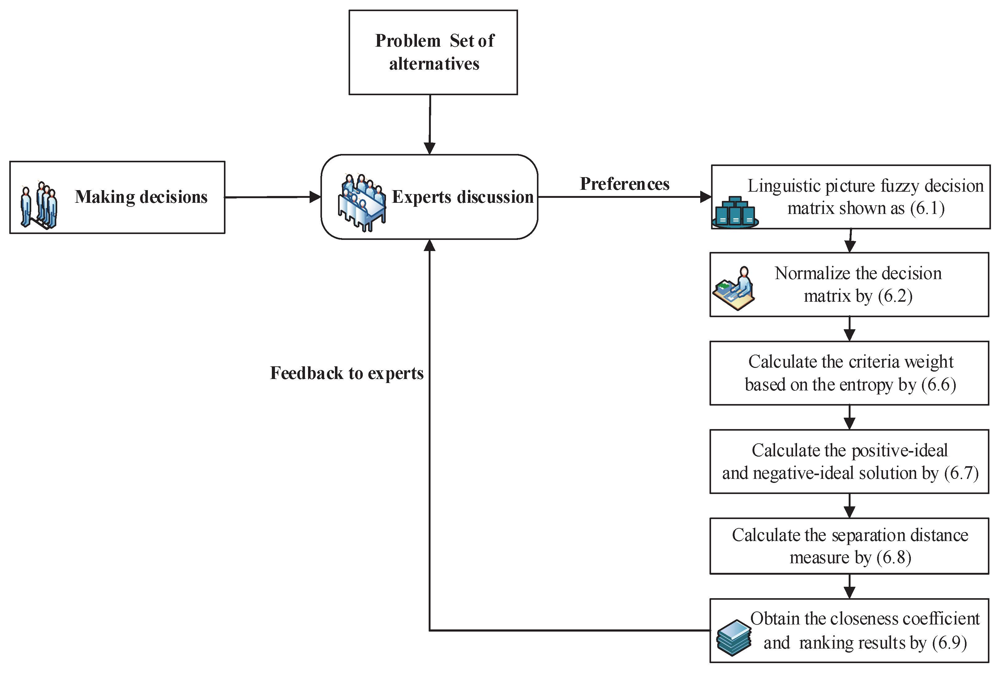
In general, the flow diagram of the proposed TOPSIS method is depicted in Figure 1.

Figure 1. The flow diagram of the proposed TOPSIS method.

In the following, we extend the TODIM method to the proposed distance measure under linguistic picture fuzzy decision environment, and the steps of the algorithm are given as follows.

Step 1 and Step 2 are the same as TOPSIS method, and here we do not give the specific steps.

Step 3: Calculate the relative weight of each criteria.

To compare the evaluation of the alternatives with different criteria, we consider the relative weight of the criterion. Assume that ${\omega }_{rj}$ is the weight of criterion $C_j$ relative to $C_r$, which can be calculated by the following formula:

$${\omega }_{rj}=\frac{{\omega }_j}{{\omega }_r},j=1,2,\dots ,n,$$

(14)

where ${\omega }_r=max\left\{{\omega }_j\right|j=1,2,\dots ,n\}$.

Step 4: Calculate the overall dominance degree of the alternative $A_i$ over alternative $A_k$ under criterion $C_j$, which is represented as follows:

$$\delta (A_i,A_k)=\sum _{j=1}^n{\varphi }_j(A_i,A_k),i,k=1,2,\dots ,m,$$

(15)

where ${\varphi }_j(A_i,A_k)$ is the dominance degree of the alternative $A_i$ over $A_k$ under criterion $C_j$, and

$${\varphi }_j(A_i,A_k)=\left\{\begin{array}{cc}\sqrt[q]{\frac{{\omega }_{rj}}{{\sum }_{j=1}^n{\omega }_{rj}}{\left(d_{1HNY}(A_{ij},A_{kj})\right)}^q},\hfill & A_{ij}>A_{kj};\hfill \\ 0,\hfill & A_{ij}=A_{kj};\hfill \\ -\frac{1}{\eta }\sqrt[q]{\frac{{\sum }_{j=1}^n{\omega }_{rj}}{{\omega }_{rj}}{\left(d_{1HNY}(A_{ij},A_{kj})\right)}^q},\hfill & A_{ij}<A_{kj}.\hfill \end{array}\right.$$

(16)

The hybrid linguistic picture distance $d_{1HNY}(A_{ij},A_{kj})$ denotes the distance measure between $A_{ij}$ and $A_{kj}$, and the comparison result between $A_{ij}$ and $A_{kj}$ is determined by Definition 9. The parameter $q(q\ge 1)$ is a regulating variable that can be determined by the decision maker’s preference, and the parameter $\eta$ represents the attenuation factor of the loss.

Step 5: Calculate the overall dominance degree of the alternatives $A_i$, which is obtained by

$$\mathsf{\Psi }\left(A_i\right)=\frac{{\sum }_{k=1}^m\delta (A_i,A_k)-{\displaystyle \underset{i}{min}}\left\{{\sum }_{k=1}^m\delta (A_i,A_k)\right\}}{{\displaystyle \underset{i}{max}}\left\{{\sum }_{k=1}^m\delta (A_i,A_k)\right\}-{\displaystyle \underset{i}{min}}\left\{{\sum }_{k=1}^m\delta (A_i,A_k)\right\}},$$

(17)

where $i=1,2,\cdots ,m$.

Step 6: Ranking the alternatives according to the value of $\mathsf{\Psi }\left(A_i\right)$, the bigger $\mathsf{\Psi }\left(A_i\right)$ is, the better alternative will be.

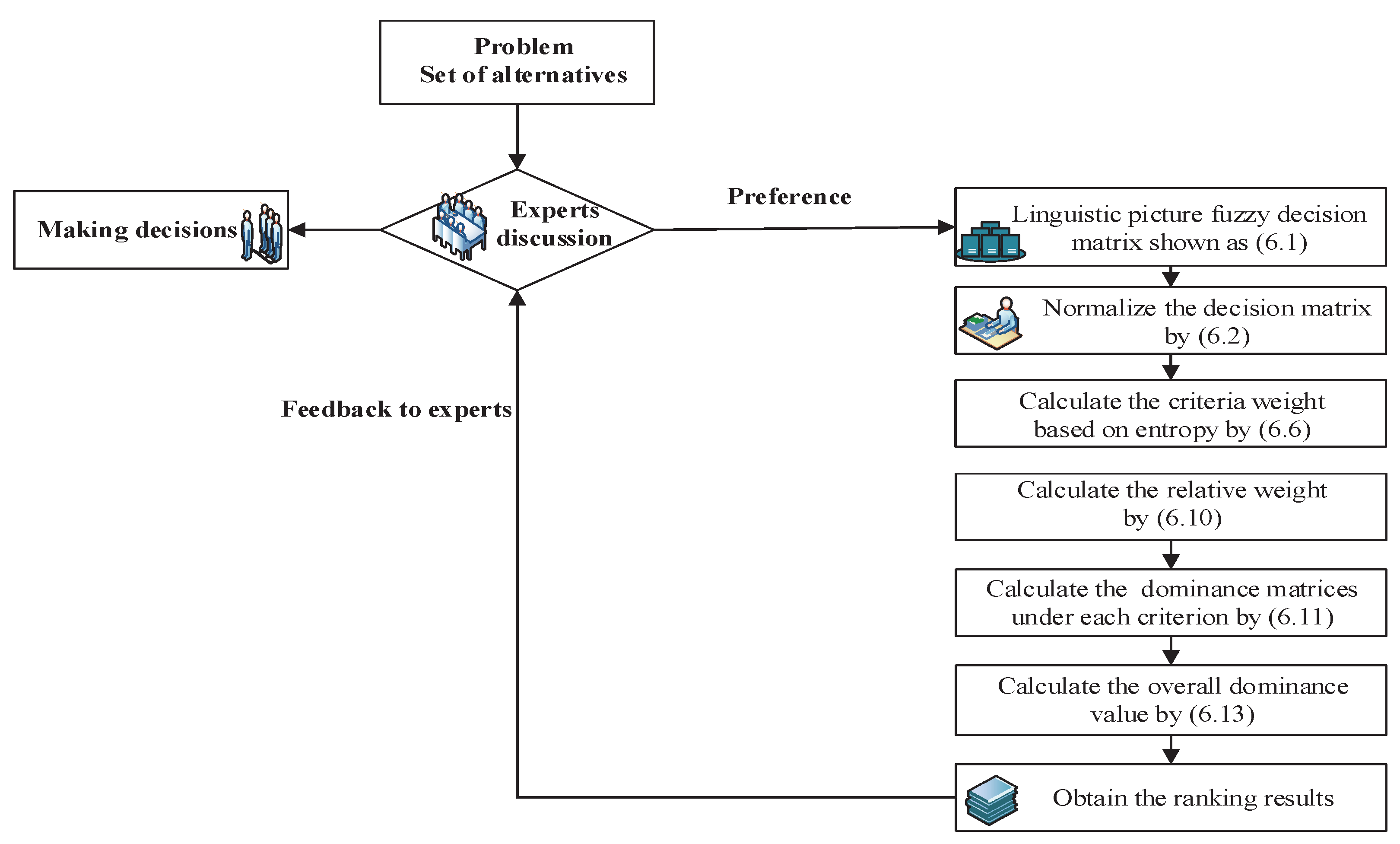
The flow diagram of the proposed TODIM method is depicted in Figure 2.

Figure 2. The flow diagram of the proposed TODIM method.

7. Numerical Example

In this section, we give a numerical example (adapted from Chan and Kumar [42]) to illustrate the feasibility and effectiveness of the proposed methods. The comparisons with other existing methods are also discussed to show their advantages.

7.1. Background

A manufacturer wants to choose the best global supplier for the most critical parts used in its production process. Four suppliers $A_i(i=1,2,3,4)$ are evaluated based on the criterion $C_j(j=1,2,\dots ,5)$, and the criterion $C_j(j=1,2,\dots ,5)$ stands for “overall cost of the product”, “quality of the product”, “service performance of supplier”, “supplier’s profile” and “risk factor”, respectively. The evaluation information of the suppliers $A_i(i=1,2,3,4)$ is represented by the LPFN $(s_{{\alpha }_i},s_{{\beta }_i},s_{{\theta }_i})\in S_{[0,2\tau ]}=S_{[0,8]}$, and the corresponding linguistic picture fuzzy decision matrix A is shown in Table 1, where the linguistic term S = {$s_0$ = extremely poor, $s_1$ = very poor, $s_2$ = poor, $s_3$ = slightly poor, $s_4$ = fair, $s_5$ = slightly good, $s_6$ = good, $s_7$ = very good, $s_8$ = extremely good}.

Table 1. The linguistic picture fuzzy decision matrix A.

	${\mathit{C}}_1$	${\mathit{C}}_2$	${\mathit{C}}_3$	${\mathit{C}}_4$	${\mathit{C}}_5$
$A_1$	$(s_6,s_1,s_1)$	$(s_4,s_3,s_1)$	$(s_4,s_3,s_1)$	$(s_5,s_2,s_1)$	$(s_4,s_3,s_1)$
$A_2$	$(s_4,s_3,s_1)$	$(s_4,s_2,s_2)$	$(s_4,s_2,s_1)$	$(s_5,s_1,s_1)$	$(s_6,s_1,s_1)$
$A_3$	$(s_4,s_2,s_1)$	$(s_5,s_2,s_1)$	$(s_6,s_1,s_1)$	$(s_4,s_2,s_1)$	$(s_4,s_1,s_2)$
$A_4$	$(s_4,s_1,s_2)$	$(s_5,s_1,s_1)$	$(s_3,s_2,s_1)$	$(s_4,s_3,s_1)$	$(s_3,s_2,s_2)$

In the following, we apply the proposed TOPSIS and TODIM methods in Section 6 to solve the above multi-criteria decision-making problem, respectively.

7.2. TOPSIS Method

In this subsection, the TOPSIS method based on linguistic picture fuzzy entropy proposed in Section 6.1 is used to select the most appropriate alternative.

Step 1: Normalize the linguistic picture fuzzy decision matrix A.

Because the criteria $C_1$ and $C_5$ are the cost-type, we transform the matrix A to normalized matrix $\tilde{A}$ by (6), the corresponding normalized decision matrix $\tilde{A}$ is obtained in Table 2.

Table 2. The normalized linguistic picture fuzzy decision matrix $\tilde{A}$.

	${\mathit{C}}_1$	${\mathit{C}}_2$	${\mathit{C}}_3$	${\mathit{C}}_4$	${\mathit{C}}_5$
$A_1$	$(s_1,s_1,s_6)$	$(s_4,s_3,s_1)$	$(s_4,s_3,s_1)$	$(s_5,s_2,s_1)$	$(s_1,s_3,s_4)$
$A_2$	$(s_1,s_3,s_4)$	$(s_4,s_2,s_2)$	$(s_4,s_2,s_1)$	$(s_5,s_1,s_1)$	$(s_1,s_1,s_6)$
$A_3$	$(s_1,s_2,s_4)$	$(s_5,s_2,s_1)$	$(s_6,s_1,s_1)$	$(s_4,s_2,s_1)$	$(s_2,s_1,s_4)$
$A_4$	$(s_2,s_1,s_4)$	$(s_5,s_1,s_1)$	$(s_3,s_2,s_1)$	$(s_4,s_3,s_1)$	$(s_2,s_2,s_3)$

Step 2: Calculate the objective weights of each criteria based on linguistic picture fuzzy entropy.

We apply the linguistic picture fuzzy entropy to calculate the weights of each criteria and the entropy value matrix is obtained in Table 3. The weight vector $\omega =({\omega }_1,{\omega }_2,{\omega }_3,{\omega }_4,{\omega }_5)=(0.2021,0.1995,0.1995,0.2021,0.1986)$ is obtained by using Equations (9) and (10).

Table 3. The entropy matrix of $\tilde{A}$.

	${\mathit{C}}_1$	${\mathit{C}}_2$	${\mathit{C}}_3$	${\mathit{C}}_4$	${\mathit{C}}_5$
$A_1$	0.375	0.625	0.625	0.5	0.625
$A_2$	0.625	0.75	0.675	0.5	0.375
$A_3$	0.625	0.5	0.375	0.625	0.625
$A_4$	0.625	0.5	0.75	0.625	0.875

Step 3: Determine the linguistic picture fuzzy positive-ideal solution $A^{+}$ and negative-ideal solution $A^{-}$, respectively, and the results are obtained as follows:

$$\begin{array}{c}\hfill A^{+}=\{(s_2,s_1,s_4),(s_5,s_2,s_1),(s_6,s_1,s_1),(s_5,s_2,s_1),(s_2,s_2,s_3)\},\\ \hfill A^{-}=\{(s_1,s_1,s_6),(s_4,s_2,s_2),(s_3,s_2,s_1),(s_4,s_2,s_1),(s_1,s_1,s_6)\}.\end{array}$$

Step 4: Based on the obtained weight of the criteria in Step 2, we utilize the hybrid linguistic picture fuzzy distance measure $d_{1HWY}(\lambda =3)$ defined in (4) to calculate the separation distance between $A_i$ and $A^{+}$, $A_i$ and $A^{-}$, respectively, the results are obtained in Table 4.

Table 4. The separation distance of each alternative.

	${\mathit{A}}_1$	${\mathit{A}}_2$	${\mathit{A}}_3$	${\mathit{A}}_4$
$D_i^{+}$	0.1862	0.2385	0.1024	0.2055
$D_i^{-}$	0.1607	0.1313	0.2366	0.2239

Step 5: Calculate the closeness coefficient of each alternative as follows:

$$\begin{array}{c}\hfill {\rho }_1=0.4633,{\rho }_2=0.3551,{\rho }_3=0.6979,{\rho }_4=0.5215,\end{array}$$

so the ranking order is $A_3\succ A_4\succ A_1\succ A_2$, that is to say, the best alternative is $A_3$.

7.3. TODIM Method

In the following, we apply the TODIM method to deal with the same numerical example, and the calculation steps are given as follows:

The results of Step 1 and Step 2 are the same as Section 7.2.

Step 3: Calculate the relative weight.

Since $\omega =(0.2021,0.1995,0.1995,0.2021,0.1968)$, then ${\omega }_r={\omega }_1={\omega }_3=0.2021.$ According to (14), we can obtain the relative weight as follows: ${\omega }_{11}=1$, ${\omega }_{12}=0.9868,$${\omega }_{13}=0.9868$, ${\omega }_{14}=1$ and ${\omega }_{15}=0.9738.$

Step 4: Calculate the overall dominance degree of the alternative $A_i$ over alternative $A_k$ under criteria $C_j$.

We assume $\eta =2$ and apply the hybrid generalized distance measure $d_{1HWY}(\lambda =3)$ defined in (4) to calculate the overall dominance degree of the alternative $A_i$ over alternative $A_k$ under criteria $C_j(j=1,2,3,4,5)$, which are obtained as follows:

$$\begin{array}{c}\hfill {\varphi }_1(A_i,A_k)=\left(\begin{array}{cccc}0& -0.2780& -0.2501& -0.2501\\ 0.1124& 0& 0.0511& -0.2561\\ 0.1035& -0.1263& 0& -0.1390\\ 0.1035& 0.1035& 0.0562& 0\end{array}\right),\end{array}$$

$$\begin{array}{c}\hfill {\varphi }_2(A_i,A_k)=\left(\begin{array}{cccc}0& 0.0558& -0.1399& -0.2578\\ -0.1399& 0& -0.1399& -0.1507\\ 0.0558& 0.0558& 0& 0.0507\\ 0.1028& 0.0601& -0.1271& 0\end{array}\right),\end{array}$$

$$\begin{array}{c}\hfill {\varphi }_3(A_i,A_k)=\left(\begin{array}{cccc}0& 0.0507& -0.2799& 0.0558\\ -0.1271& 0& -0.2578& 0.0507\\ 0.1117& 0.1028& 0& 0.1528\\ -0.1399& -0.1271& -0.3830& 0\end{array}\right),\end{array}$$

$$\begin{array}{c}\hfill {\varphi }_4(A_i,A_k)=\left(\begin{array}{cccc}0& 0.0511& 0.0511& 0.0562\\ -0.1263& 0& 0.0562& 0.1035\\ -0.1263& -0.1390& 0& -0.1263\\ -0.1391& -0.2561& 0.0511& 0\end{array}\right),\end{array}$$

$$\begin{array}{c}\hfill {\varphi }_5(A_i,A_k)=\left(\begin{array}{cccc}0& 0.1109& -0.2595& -0.1518\\ -0.2818& 0& -0.2595& -0.3871\\ 0.1021& 0.1021& 0& -0.1409\\ 0.0597& 0.1524& 0.0555& 0\end{array}\right),\end{array}$$

$$\begin{array}{c}\hfill \delta (A_i,A_k)=\left(\begin{array}{cccc}0& -0.0095& -0.8843& -0.5537\\ -0.5627& 0& -0.5499& -0.6397\\ 0.2468& -0.0046& 0& -0.2027\\ -0.0129& -0.0672& -0.3473& 0\end{array}\right).\end{array}$$

Step 5: Using (17) to calculate the overall dominance degree of the alternative $A_i$, we have $\mathsf{\Psi }\left(A_1\right)=0.1701,\mathsf{\Psi }\left(A_2\right)=0,\mathsf{\Psi }\left(A_3\right)=1,\mathsf{\Psi }\left(A_4\right)=0.7394$.

Step 6: Ranking the alternatives based on the overall dominance degree of the alternative, it is obvious that the ranking order of the alternatives is $A_3\succ A_4\succ A_1\succ A_2$, so $A_3$ is the best alternative.

7.4. Comparison Analysis with Other Existing Methods

In this subsection, in order to verify the effectiveness of the proposed methods for solving the multi-criteria decision-making problems, we utilize the aggregation operators, the different distance measures, and other existing methods to calculate the same numerical example, and the results are given in Table 5.

Table 5. Comparison results with other distance measures and existing methods.

Approach	Ranking   Results
Approach from Krohling et al. [43]	$A_3\succ A_4\succ A_1\succ A_2$
Approach from Boran et al. [44]	$A_3\succ A_4\succ A_1\succ A_2$
Approach based on $LPFWA$ operator	$A_3\succ A_4\succ A_1\succ A_2$
Approach based on $LPFWG$ operator	$A_4\succ A_3\succ A_1\succ A_2$
$TOPSIS$ method based on $d_{3\omega }$ (shown in Appendix A)	$A_3\succ A_4\succ A_1\succ A_2$
$TOPSIS$ method based on $d_{3wH}$ (shown in Appendix A)	$A_3\succ A_4\succ A_1\succ A_2$
$TODIM$ method based on $d_{3\omega }$	$A_3\succ A_4\succ A_1\succ A_2$
$TODIM$ method based on $d_{3wH}$	$A_3\succ A_4\succ A_1\succ A_2$

From Table 5, we can see that the ranking results of the proposed methods are the same as the method of Krohling et al. [43] and Boran et al. [44], which can demonstrate the feasibility of the proposed TOPSIS and TODIM methods based on the linguistic picture fuzzy entropy in this paper.

If we apply the LPFWA operator and LPFWG operator to aggregate the decision information, respectively, we can obtain $A_1^{{}^{\prime }}=LPFWA({\tilde{A}}_{11},{\tilde{A}}_{12},{\tilde{A}}_{13},{\tilde{A}}_{14},{\tilde{A}}_{15})=(s_{3.2820},s_{2.2136},s_{1.8869}),A_2^{{}^{\prime }}=(s_{3.2820},s_{1.6464},s_{2.1621}),A_3^{{}^{\prime }}=(s_{4.0111},s_{1.5196},s_{1.7384})$ and $A_4^{{}^{\prime }}=(s_{3.3579},s_{1.6433},s_{1.6428})$. Based on the score function of LPFS, we can obtain $A_3\ge A_4\ge A_1\ge A_2$. Similarly, we apply the LPFWG operator to obtain the aggregated decision values as follows: $A_1^{{}^{\prime }}=(s_{2.4070},s_{2.4472},s_{3.1324}),$$A_2^{{}^{\prime }}=(s_{2.4070},s_{1.8503},s_{3.2625})$, $A_3^{{}^{\prime }}=(s_{2.9895},s_{1.6220},s_{2.4005})$ and $A_4^{{}^{\prime }}=(s_{2,9949},s_{1.8477},s_{2.1491})$. Using the score function of LPFS, we have $A_4\ge A_3\ge A_1\ge A_2$. Obviously, the ranking result of the alternatives based on LPFWG operator is different from that obtained by the proposed method in this paper. The differences are the ranking orders between $A_3$ and $A_4$. The main reason is that the operation of geometric operator does not satisfy the closure of operation and may cause the loss of decision information.

Compared with other existing methods, the proposed decision-making methods have some advantages in solving multi-criteria decision-making problems. In the methods of Krohling [43] and Boran [44] et al., they consider the TODIM and TOPSIS methods in IFS, which cannot meet the needs of decision-making problems involving more answers of types. We can know it from the following aspects.

Firstly, the proposed LPFS is a generalized form of IFS by incorporating the neutral membership degree, which can deal with the decision information better under uncertain conditions. Secondly, the proposed LPFS overcomes the limitations of PFS that represents the decision information with numerical value, which express the evaluation information with LTS that is closer to human cognitive ability. Thirdly, considering the weight of criteria is an important component of multi-criteria decision-making problem, we propose the linguistic picture fuzzy entropy to calculate the objective weight of criteria and reduce the randomness in decision-making process, which can improve the rationality of decision-making results. The proposed hybrid distance measures between LPFSs are constructed based on the geometric interpretation of LPFSs in some extent, which is more suitable for comparing the alternatives.

7.5. Sensitivity Analysis

In this subsection, we make the sensitivity analysis of parameters in the proposed TOPSIS and TODIM methods.

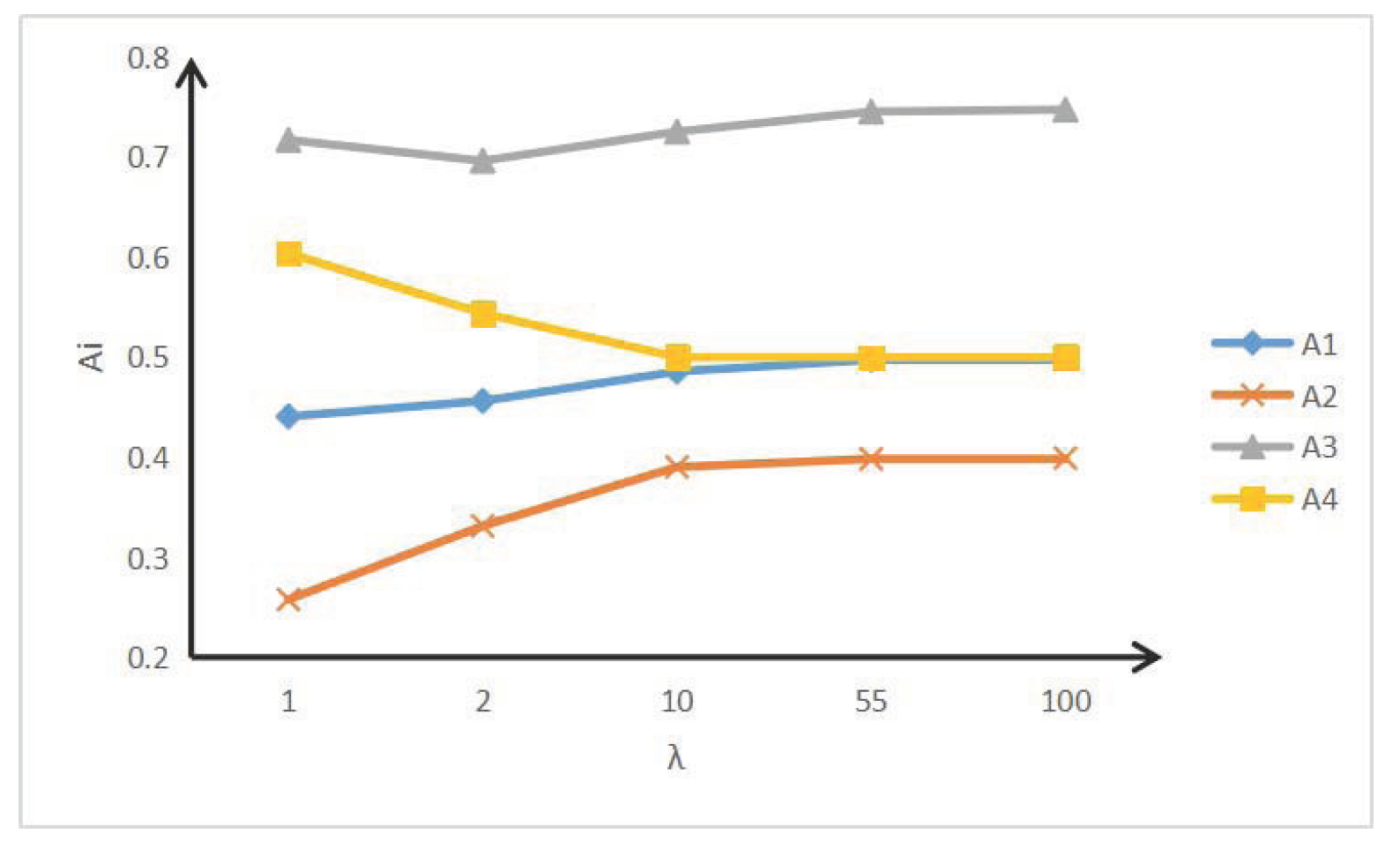
Firstly, in the TOPSIS method between LPFSs, we consider the influence of the parameter $\lambda$ in hybrid distance measure $d_{1WHY}$. Letting $\lambda =1,2,10,55,100$, we can obtain the ranking results with different $\lambda$, which are given in Table 6, and the corresponding change diagram is shown in Figure 3. According to Figure 3, we can see that the calculation values of $A_1,A_2$ and $A_3$ are increasing as $\lambda$ increases. However, the calculation values of $A_4$ are decreasing as the value of $\lambda$ increases, which shows that the change of $\lambda$ in the distance measure may affect the decision makers. We can also see that the ranking order of the alternatives is $A_3\succ A_4\succ A_2\succ A_1$ for different $\lambda$, which illustrates the stability of the proposed TOPSIS method between LPFSs for different distance measures.

Table 6. Ranking results obtained by $TOPSIS$ method with different $\lambda$.

$\mathit{\lambda }$	${\mathit{\rho }}_1$	${\mathit{\rho }}_2$	${\mathit{\rho }}_3$	${\mathit{\rho }}_4$	Ranking   Results
$\lambda =1$	0.4470	0.2577	0.7172	0.6037	$A_3\succ A_4\succ A_1\succ A_2$
$\lambda =2$	0.4562	0.3312	0.6963	0.5438	$A_3\succ A_4\succ A_1\succ A_2$
$\lambda =10$	0.4856	0.3902	0.7255	0.5001	$A_3\succ A_4\succ A_1\succ A_2$
$\lambda =55$	0.4974	0.3983	0.7455	0.4999	$A_3\succ A_4\succ A_1\succ A_2$
$\lambda =100$	0.4986	0.3991	0.7475	0.5000	$A_3\succ A_4\succ A_1\succ A_2$

Figure 3. The ranking results by $TOPSIS$ with different $\lambda$.

Secondly, we consider the influence of three parameters $\lambda ,\eta$ and q in the proposed TODIM method between LPFSs.

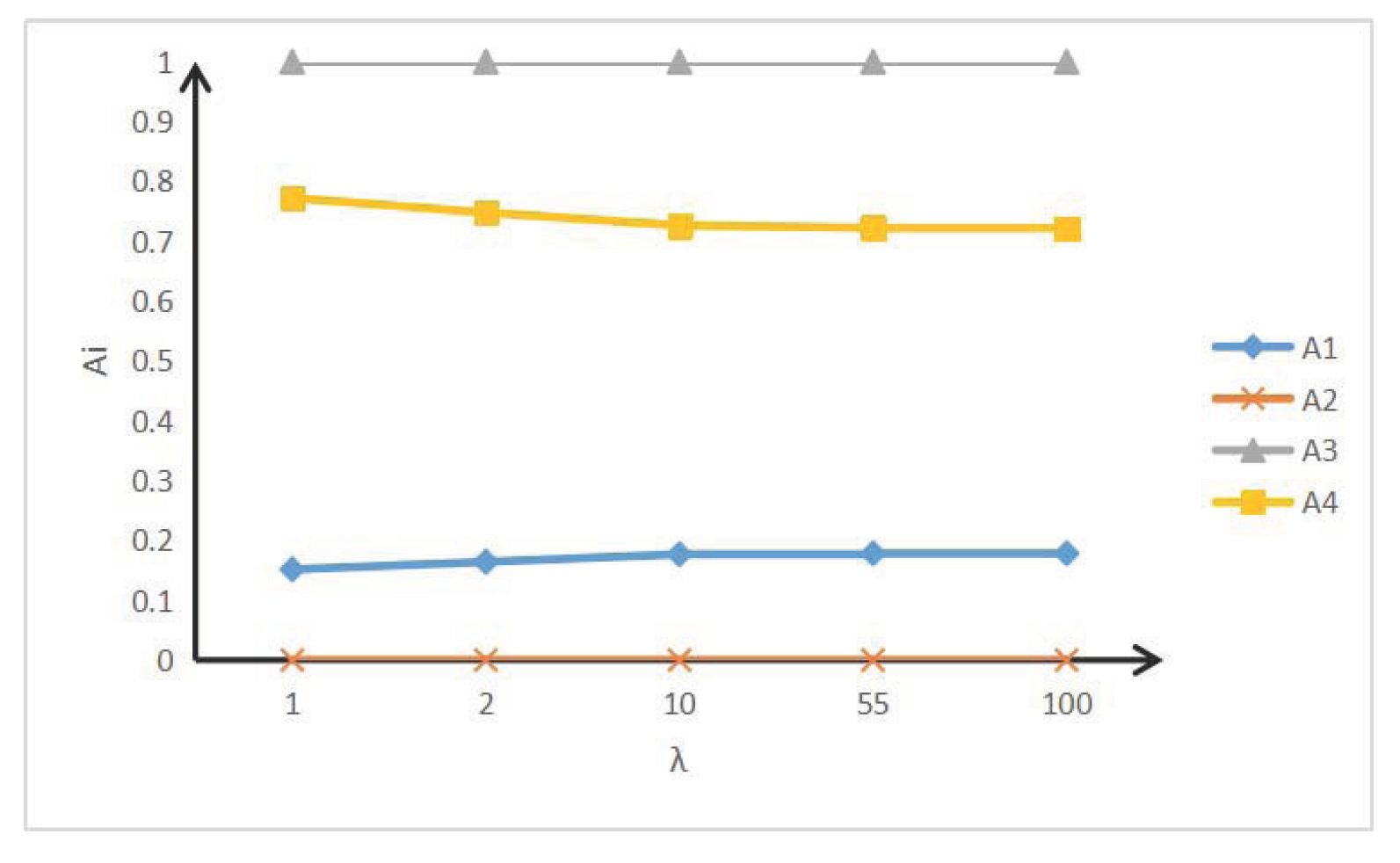
(1) We calculate the ranking results of the alternatives with different $\lambda$ in hybrid distance measure $d_{1WHY}$. Assuming $\eta =2$ and $q=2$, let $\lambda =1,2,10,55,100$, the calculation results of the alternatives with different $\lambda$ are obtained in Table 7, the corresponding graph with change of parameter $\lambda$ is shown in Figure 4. From Figure 4, we can see that the ranking results is always $A_3\succ A_4\succ A_1\succ A_2$, which also shows the stability of parameter $\lambda$ in the proposed TODIM method between LPFSs for different distance measures.

Table 7. Ranking results obtained by $TODIM$ method with $\eta =2$, $q=2$ and different $\lambda$.

$\mathit{\lambda }$	${\mathsf{\Psi }}_1$	${\mathsf{\Psi }}_2$	${\mathsf{\Psi }}_3$	${\mathsf{\Psi }}_4$	Ranking   Results
$\lambda =1$	0.1516	0	1	0.7723	$A_3\succ A_4\succ A_1\succ A_2$
$\lambda =2$	0.1641	0	1	0.7480	$A_3\succ A_4\succ A_1\succ A_2$
$\lambda =10$	0.1769	0	1	0.7267	$A_3\succ A_4\succ A_1\succ A_2$
$\lambda =55$	0.1783	0	1	0.7223	$A_3\succ A_4\succ A_1\succ A_2$
$\lambda =100$	0.1784	0	1	0.7218	$A_3\succ A_4\succ A_1\succ A_2$

Figure 4. The ranking results by $TODIM$ method with $\eta =2$, $q=2$ and different $\lambda$.

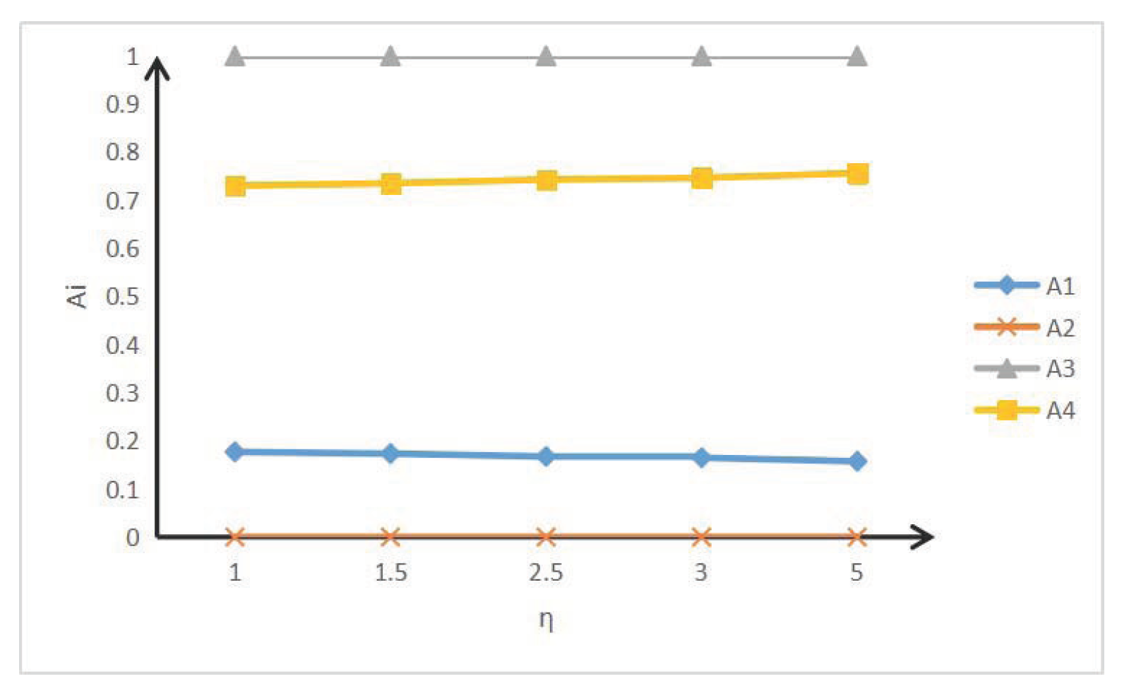
(2) We consider the influence of the parameter $\eta$ in the TODIM method, which represents the sensitive coefficient of risk aversion. Assuming $\lambda =3$ and $q=2$, let $\eta =1,1.5,2.5,3,5$, the ranking results with different $\eta$ are shown in Table 8, we know the ranking order of the alternatives is $A_3\succ A_4\succ A_1\succ A_2$. The corresponding graph with change of parameter $\eta$ is shown in Figure 5, and it is clear that the ranking results are stable for different $\eta$, which illustrates that the decision maker is not sensitive to risk aversion.

Table 8. Ranking results obtained by $TODIM$ method with $\lambda =3$, $q=2$ and different $\eta$.

$\mathit{\eta }$	${\mathsf{\Psi }}_1$	${\mathsf{\Psi }}_2$	${\mathsf{\Psi }}_3$	${\mathsf{\Psi }}_4$	Ranking   Results
$\eta =1$	0.1770	0	1	0.7303	$A_3\succ A_4\succ A_1\succ A_2$
$\eta =1.5$	0.1734	0	1	0.7351	$A_3\succ A_4\succ A_1\succ A_2$
$\eta =2.5$	0.1674	0	1	0.7430	$A_3\succ A_4\succ A_1\succ A_2$
$\eta =3$	0.1650	0	1	0.7463	$A_3\succ A_4\succ A_1\succ A_2$
$\eta =5$	0.1574	0	1	0.7564	$A_3\succ A_4\succ A_1\succ A_2$

Figure 5. The ranking results by $TODIM$ with $\lambda =3,q=2$ and different $\eta$.

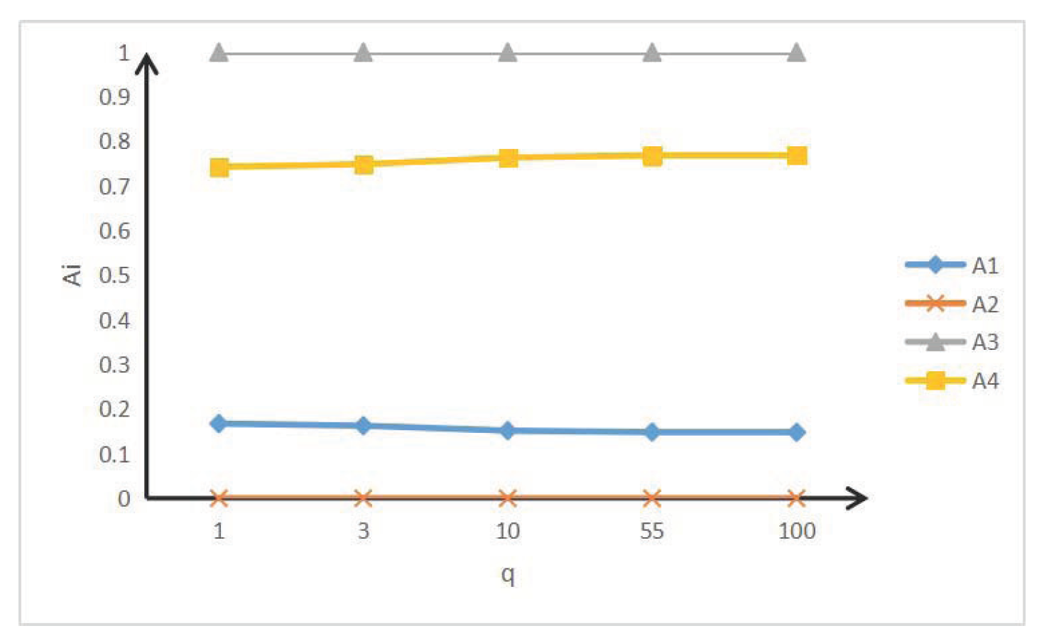
(3) The parameter q in TODIM method is a regulation variable, which represents the preference of decision makers. Now, we consider the influence of q on decision results. Assuming $\lambda =3$ and $\eta =2$, let $q=1,3,10,55,100$. The calculation results are obtained in Table 9 and the change graph corresponding to q is shown in Figure 6. According to Table 9, we can see that the ranking result of the alternatives is $A_3\succ A_4\succ A_1\succ A_2$, and the change of parameter q does not change the stability of the TODIM method, which can also be illustrated from Figure 6.

Table 9. Ranking results obtained by $TODIM$ method with $\eta =2$, $\lambda =3$ and different q.

q	${\mathsf{\Psi }}_1$	${\mathsf{\Psi }}_2$	${\mathsf{\Psi }}_3$	${\mathsf{\Psi }}_4$	Ranking   Results
$q=1$	0.1674	0	1	0.7430	$A_3\succ A_4\succ A_1\succ A_2$
$q=3$	0.1627	0	1	0.7486	$A_3\succ A_4\succ A_1\succ A_2$
$q=10$	0.1517	0	1	0.7635	$A_3\succ A_4\succ A_1\succ A_2$
$q=55$	0.1482	0	1	0.7686	$A_3\succ A_4\succ A_1\succ A_2$
$q=100$	0.1479	0	1	0.7691	$A_3\succ A_4\succ A_1\succ A_2$

Figure 6. The ranking results by $TODIM$ with $\lambda =3,\eta =2$ and different q.

8. Conclusions

In this paper, we proposed the LPFS based on PFS and LTS, where the positive-membership, the neutral-membership, and the negative-membership are represented by linguistic variables, and the LPFS can deal with the vague and imprecise information in qualitative environment. Furthermore, the operation rules of LPFSs, the LPFWA operator, and LPFWG operator are developed. Then, we define some distance measures between LPFSs, and the TOPSIS method and TODIM method are developed to the proposed distance measures based on the linguistic picture fuzzy entropy. Finally, an illustrative example is given to illustrate the effectiveness of the proposed methods, and the comparative analysis with other existing methods and sensitivity analysis of the proposed methods are also discussed.

Although the proposed linguistic picture fuzzy set can solve the multi-criteria decision-making problems, which still has the following limitations: (1) The linguistic term sets considered in this paper are calculated based on the subscript of linguistic terms and the subscript is integer, which may cause a loss of evaluation information. (2) The aggregated operators may not be a linguistic term set, which is unreasonable and counterintuitive. (3) The proposed hybrid distance measure only considered the Hausdorff distance measure based on the maximum value, which is susceptible to the extreme values and it may cause the inaccurate ranking result in the multi-criteria decision-making problems with extreme evaluation information.

In the future, in order to overcome the above limitations, we will take further studies from the following aspects: (1) The different semantic situations with linguistic scale function can be considered into the picture fuzzy sets, and it can be extended to the uncertain linguistic term set. (2) How to define a new aggregated operator that satisfies the closure of linguistic picture fuzzy set. (3) The proposed hybrid distance measure can take the mean and variance of linguistic picture fuzzy set into consideration and it can be extended to the continuous distance measure. Furthermore, the proposed method can be applied to practical decision-making problems such as pattern recognition, medical diagnosis et al.

References

1. Zadeh, L.A. Fuzzy sets. Inf. Control 1965, 8, 338–353. [Google Scholar] [CrossRef] [Green Version]
2. Atanassov, K.T. Intuitionistic fuzzy set. Fuzzy Sets Syst. 1986, 20, 87–96. [Google Scholar] [CrossRef]
3. Cuong, B.C. Picture fuzzy sets. J. Comput. Sci. Cybern. 2014, 30, 409–420. [Google Scholar]
4. Zadeh, L.A. The concept of a linguistic variable and its application to approximate reasoning-I. Inf. Sci. 1975, 8, 199–249. [Google Scholar] [CrossRef]
5. Zadeh, L.A. The concept of a linguistic variable and its application to approximate reasoning-II. Inf. Sci. 1975, 8, 301–357. [Google Scholar] [CrossRef]
6. Zadeh, L.A. The concept of a linguistic variable and its application to approximate reasoning-III. Inf. Sci. 1975, 9, 43–80. [Google Scholar] [CrossRef]
7. Herrera, F.; Herrera-Viedma, E. Linguistic decision analysis: Steps for solving decision problems under linguistic information. Fuzzy Sets Syst. 2000, 115, 67–82. [Google Scholar] [CrossRef]
8. Herrera, F.; Herrera-Viedma, E.; Martinez, L. A Fuzzy Linguistic Methodology to Deal With Unbalanced Linguistic Term Sets. IEEE Trans. Fuzzy Syst. 2008, 16, 354–370. [Google Scholar] [CrossRef]
9. Martinezlopez, L.; Ruan, D.; Herrera, F.; Herreraviedma, E.; Wang, P.P. Linguistic decision-making: Tools and applications. Inf. Sci. 2009, 179, 2297–2298. [Google Scholar] [CrossRef]
10. Rodríguez, R.M.; MartıNez, L.; Herrera, F. A group decision-making model dealing with comparative linguistic expressions based on hesitant fuzzy linguistic term sets. Inf. Sci. 2013, 241, 28–42. [Google Scholar] [CrossRef]
11. Liao, H.; Xu, Z.; Zeng, X.J.; Merigó, J.M. Qualitative decision-making with correlation coefficients of hesitant fuzzy linguistic term sets. Knowl. Based Syst. 2015, 76, 127–138. [Google Scholar] [CrossRef]
12. Chen, Z.; Liu, P.; Pei, Z. An approach to multiple attribute group decision-making based on linguistic intuitionistic fuzzy numbers. Int. J. Comput. Intell. Syst. 2015, 8, 747–760. [Google Scholar] [CrossRef] [Green Version]
13. Ashraf, S.; Mehmood, T.; Abdullah, S.; Khan, Q. Picture fuzzy linguistic sets and their applications for multi-attribute group. Nucleus 2018, 55, 66–73. [Google Scholar]
14. Zhang, X.; Wang, J.; Hu, J. On novel operational laws and aggregation operators of picture 2-tuple linguistic information for MCDM problems. Int. J. Fuzzy Syst. 2018, 20, 958–969. [Google Scholar] [CrossRef]
15. Liu, P.; Zhang, X. A novel picture fuzzy linguistic aggregation operator and its application to group decision-making. Cogn. Comput. 2018, 10, 242–259. [Google Scholar] [CrossRef]
16. Wei, G.; Alsaadi, F.E.; Hayat, T.; Alsaedi, A. Picture 2-tuple linguistic aggregation operators in multiple attribute decision-making. Soft Comput. 2018, 22, 989–1002. [Google Scholar] [CrossRef]
17. Wu, X.; Liao, H. An approach to quality function deployment based on probabilistic linguistic term sets and ORESTE method for multi-expert multi-criteria decision-making. Inf. Fusion 2018, 43, 13–26. [Google Scholar] [CrossRef]
18. Wei, G. Picture fuzzy cross-entropy for multiple attribute decision-making problems. J. Bus. Econ. Manag. 2016, 17, 491–502. [Google Scholar] [CrossRef] [Green Version]
19. Wei, G. Picture 2-Tuple Linguistic Bonferroni Mean Operators and Their Application to Multiple Attribute Decision Making. Int. J. Fuzzy Syst. 2017, 19, 997–1010. [Google Scholar] [CrossRef]
20. Wang, C.; Zhou, X.; Tu, H.; Tao, S. Some geometric aggregation operators based on picture fuzzy sets and their application in multiple attribute decision-making. Ital. J. Pure Appl. Math. 2017, 37, 477–492. [Google Scholar]
21. Wang, L.; Zhang, H.; Wang, J.; Li, L. Picture fuzzy normalized projection-based VIKOR method for the risk evaluation of construction project. Appl. Soft Comput. 2018, 64, 216–226. [Google Scholar] [CrossRef]
22. Singh, P. Correlation coefficients for picture fuzzy sets. J. Intell. Fuzzy Syst. 2015, 28, 591–604. [Google Scholar] [CrossRef]
23. Wei, G. Picture fuzzy aggregation operators and their application to multiple attribute decision-making. J. Intell. Fuzzy Syst. 2017, 33, 713–724. [Google Scholar] [CrossRef]
24. Son, L.H. Generalized picture distance measure and applications to picture fuzzy clustering. Appl. Soft Comput. 2016, 46, 284–295. [Google Scholar] [CrossRef]
25. Son, L.H. Measuring analogousness in picture fuzzy sets: From picture distance measures to picture association measures. Fuzzy Optim. Decis. Mak. 2017, 16, 359–378. [Google Scholar] [CrossRef]
26. Jana, C.; Senapati, T.; Pal, M.; Yager, R.R. Picture fuzzy Dombi aggregation operators: Application to MADM process. Appl. Soft Comput. 2019, 74, 99–109. [Google Scholar] [CrossRef]
27. Xu, Z.; Xia, M. Distance and similarity measures for hesitant fuzzy sets. Inf. Sci. 2011, 181, 2128–2138. [Google Scholar] [CrossRef]
28. Wang, W.; Xin, X. Distance measure between intuitionistic fuzzy sets. Pattern Recognit. Lett. 2005, 26, 2063–2069. [Google Scholar] [CrossRef]
29. Liu, D.; Chen, X.; Peng, D. Some cosine similarity measures and distance measures between q-rung orthopair fuzzy sets. Int. J. Intell. Syst. 2019, 34, 1572–1587. [Google Scholar] [CrossRef]
30. Li, D.; Zeng, W. Distance measure of Pythagorean fuzzy sets. Int. J. Intell. Syst. 2018, 33, 348–361. [Google Scholar] [CrossRef]
31. Xiao, F.; Ding, W. Divergence measure of Pythagorean fuzzy sets and its application in medical diagnosis. Appl. Soft Comput. 2019, 79, 254–267. [Google Scholar] [CrossRef]
32. Yoon, K.; Hwang, C.L. TOPSIS (Technique for Order Preference by Similarity to Ideal Solution) Ca Multiple Attribute Decision Making; Springer: Berlin, Germany, 1981. [Google Scholar]
33. Sajjad Ali Khan, M.; Abdullah, S.; Yousaf Ali, M.; Hussain, I.; Farooq, M. Extension of TOPSIS method base on Choquet integral under interval-valued Pythagorean fuzzy environment. J. Intell. Fuzzy Syst. 2018, 34, 267–282. [Google Scholar] [CrossRef]
34. Liu, D.; Liu, Y.; Chen, X. Fermatean fuzzy linguistic set and its application in multicriteria decision-making. Int. J. Intell. Syst. 2018, 34, 878–894. [Google Scholar] [CrossRef]
35. Chen, Z.-S.; Yang, Y.; Wang, X.-J.; Chin, K.-S.; Tsui, K.-L. Fostering linguistic decision-making under uncertainty: A proportional interval type-2 hesitant fuzzy TOPSIS approach based on Hamacher aggregation operators and andness optimization models. Inf. Sci. 2019, 500, 229–258. [Google Scholar] [CrossRef]
36. Gomes, L.F.; Lima, M. TODIM: Basics and apllication to multicriteria ranking of projects with environmental impacts. Found. Control Eng. 1991, 16, 113–127. [Google Scholar]
37. Gomes, L.F.; Rangel, L.S. An application of the TODIM method to the multicriteria rental evaluation of residential properties. Eur. J. Oper. Res. 2009, 193, 204–211. [Google Scholar] [CrossRef]
38. Zhang, X.; Xu, Z. The TODIM analysis approach based on novel measured functions under hesitant fuzzy environment. Knowl. Based Syst. 2014, 61, 48–58. [Google Scholar] [CrossRef]
39. Ji, P.; Zhang, H.Y.; Wang, J.Q. A projection-based TODIM method under multi-valued neutrosophic environments and its application in personnel selection. Neural Comput. Appl. 2018, 29, 221–234. [Google Scholar] [CrossRef] [Green Version]
40. Liu, D.; Liu, Y.; Wang, L. Distance measure for Fermatean fuzzy linguistic term sets based on linguistic scale function: An illustration of the TODIM and TOPSIS methods. Int. J. Intell. Syst. 2019, 34, 2807–2834. [Google Scholar] [CrossRef]
41. Xu, Z. A method based on linguistic aggregation operators for group decision-making with linguistic preference relations. Inf. Sci. 2004, 166, 19–30. [Google Scholar] [CrossRef]
42. Chan, F.T.S.; Kumar, N. Global supplier development considering risk factors using fuzzy extended AHP-based approach. Omega 2007, 35, 417–431. [Google Scholar] [CrossRef]
43. Krohling, R.A.; Pacheco, A.G.C.; Siviero, A.L.T. IF-TODIM: An intuitionistic fuzzy TODIM to multi-criteria decision-making. Knowl. Based Syst. 2013, 53, 142–146. [Google Scholar] [CrossRef]
44. Boran, F.E.; Genc, S.; Kurt, M.; Akay, D. A multi-criteria intuitionistic fuzzy group decision-making for supplier selection with TOPSIS method. Expert Syst. Appl. 2009, 36, 11363–11368. [Google Scholar] [CrossRef]