Overshoot Elimination for Control Systems with Parametric Uncertainty via a PID Controller

Abstract

One of the key performance requirements for different control systems is non-overshooting step response, so that the controllable value should not overcome the reference value within a transient process. The problem of providing a non-overshooting step response was examined in this paper. Despite much scientific research being dedicated to the overshoot elimination problem, there are little to no results regarding parametric uncertainty for the discussed problem. Consideration of parametric uncertainty, particularly in the form of interval-given parameters, is essential, since in many physical processes, electronic devices and control systems parameter values can be obtained with acceptable error, and they can vary under different conditions. The main result of our research is the development of a proportional-integral-derivative (PID)-controller tuning approach for systems with interval-given parameters that provides a non-overshooting step response for such classes of control systems. This paper investigates analytical conditions and constraints for linear time invariant (LTI) systems in order to have no overshoot, enhances them with respect to parametric uncertainty, and formulates rules for tuning choices of parameters.

1. Introduction

Regarding industrial process control, it is essential for control systems to meet the technological requirements. One of the key performance indices is overshoot. Particularly, it is essential for positioning control systems, machinery, and several thermal and chemistry processes to show no overshoot. Considering linear time invariant (LTI) systems, there has been much research worldwide that has been dedicated to the problem of overshoot. Papers [1,2] present approaches for achieving acceptable overshoot percentages on the poles domination theory basis. Several research papers, such as [3,4,5,6], have been focused on full overshoot elimination using Vandermonde-like matrices for error function representation. Other ways were proposed in [7], where the problem was considered with respect to impulse response behavior, and in [8], where minimizing of integrated absolute error (IAE) was performed. In the context of industrial process control, it is worth noting different approaches based on canonical proportional-integral-derivative (PID)-controller design methods. In particular, several results in [9,10,11,12,13] were obtained using the Ziegler–Nichols tuning method. More theoretical techniques take place as well, such as [14,15] that state and prove theorems for necessary and sufficient pole-zero configuration of the transfer function, providing a non-overshooting step response. As opposed to several analytical approaches, numeric optimization for the purpose of PID-controller tuning was regarded as well in [16,17]. Another option for controller design and tuning is the initial choice of a desired stability degree for each pole of a closed-loop control system.

Considering real-world practical applications, it is worth mentioning that systems parameters tend to be uncertain, due to measurement errors and varying conditions of functioning. Even slight parameters variations can lead to significant changes in system dynamics. Parametric uncertainty makes controller design significantly more difficult, since the controller has to meet the requirements for varying states. In addition, a robust controller tuning procedure is challenging, since many existing well-known methods become inapplicable under parametric uncertainty. Despite the high level of complexity for a robust controller design, there have been several results presented, such as [18,19] that are based on minimization of oscillatory degree for systems with interval-given parameters. Regarding systems with interval-given parameters, one of the key techniques for analysis and control design is the Kharitonov theorem. For example, the authors of [20,21,22] address vertex polynomial properties for a robust PID-control design, but in many cases, vertex polynomials do not indicate all behavior aspects of the system with interval-given parameters. Another example of a robust PID-controller design was presented in [23,24] in the context of DC converters on the mixed approach that involves Kharitonov polynomials and phase portraits.

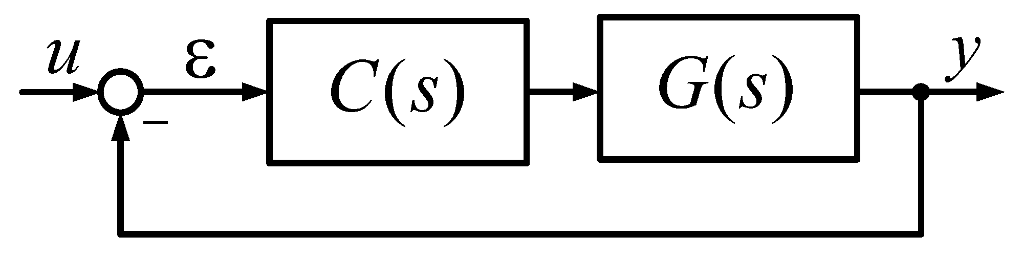
2. Materials and Methods

The presented research is conducted on the basis of the canonical closed-loop control scheme, depicted in Figure 1.

In Figure 1, $C(s)$ is the controller, $G(s)$ is the plant, and $u$, $\mathsf{\epsilon }$, and $y$ are the reference signal, error signal, and output signal respectively.

The controller, $C(s)$ in this case, is a classic PID controller, which is one of the most distributed control solutions. The PID-controller transfer function is

$$C(s)=\frac{D{s}^2+Ks+I}{s},$$

where $D$, $K$ and $I$ are the coefficients of the PID controller. The plant $G(s)$ is represented with the second-order transfer function

$$G(s)=\frac{K_P}{s^2+2\alpha s+{\alpha }^2+{\omega }^2},$$

(1)

with poles $s=\alpha \pm j\omega$ and gain $K_P$. In cases of plants with initially real poles, parameter $\omega$ is supposed to be complex with a null real part.

At the first stage of the research, a stationary LTI system was examined. The task was to figure out the rule for PID-controller coefficients, providing a non-overshoot step response. In previous research [14], one of the necessary conditions for this was that the poles of the transfer function are strictly real.

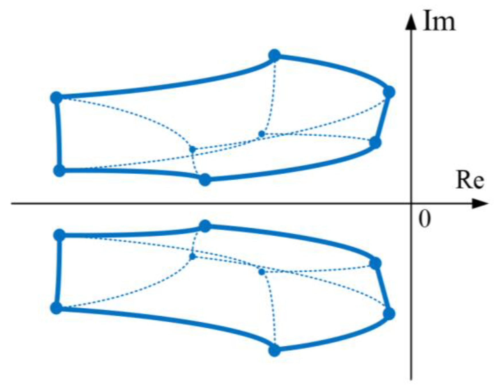
2.1. Providing Real Closed-Loop Pole Configuration

Regarding control systems structure, plant and controller transfer functions, the closed loop transfer function is

$$W(s)=\frac{K_P\left(D{s}^2+Ks+I\right)}{s^3+\left(2\alpha +D{K}_P\right)s^2+\left({\alpha }^2+{\omega }^2+K{K}_P\right)s+I{K}_P}$$

(2)

Conducting changing $D{K}_P=K^{\prime }$, $K{K}_P=K^{\prime }$, and $I{K}_P=I^{\prime }$, a characteristic equation of (2) can be represented as:

$$s^3+\left(2\alpha +D^{\prime }\right)s^2+\left({\alpha }^2+{\omega }^2+K^{\prime }\right)s+I^{\prime }$$

(3)

According to the theorem in [14], it is necessary for transfer function poles to be exclusively real. Since the roots type is defined with a discriminant sign, let us write a discriminant for (3) in the following form [25]

$$\begin{array}{l}{\mathsf{\Delta }}_{CE}\left(\alpha ,\omega ,K^{\prime },I^{\prime },D^{\prime }\right)={\left(2\alpha +D^{\prime }\right)}^2{\left({\alpha }^2+{\omega }^2+K^{\prime }\right)}^2-27{I^{\prime }}^2-\\ -4I^{\prime }{\left(2\alpha +D^{\prime }\right)}^3-4{\left({\alpha }^2+{\omega }^2+K^{\prime }\right)}^3+18I^{\prime }\left(2\alpha +D^{\prime }\right)\left({\alpha }^2+{\omega }^2+K^{\prime }\right)\end{array}$$

(4)

Substituting arbitrary real positive values of $\alpha$, $\omega$, and $K^{\prime }$ in (4), one can plot the surface of ${\mathsf{\Delta }}_{CE}\left(D^{\prime },I^{\prime }\right)$. Since only positive values of ${\mathsf{\Delta }}_{CE}$ are of interest, in the same coordinates, let us plot plane ${\mathsf{\Delta }}_{CE}=0$ to visualize constraints of the region of interest.

Figure 2 illustrates that region where ${\mathsf{\Delta }}_{CE}>0$, denoted as $\mathsf{\Omega }$, is bounded with two curves (white dashed lines). Expressing $I^{\prime }$ from (4) yields two functions describing bounding curves for $\mathsf{\Omega }$:

$$\{\begin{array}{l}{I^{\prime }}_1(\alpha ,\omega ,K^{\prime },D^{\prime })=\frac{18\alpha K^{\prime }+9D^{\prime }{K}^{\prime }+18{\omega }^2\alpha +9{\omega }^2{D}^{\prime }-12\alpha {D^{\prime }}^2-15{\alpha }^2{D}^{\prime }+2{\alpha }^3-2D^{\prime }+2\sqrt{{\left({\alpha }^2-3{\omega }^2+4\alpha D^{\prime }+{D^{\prime }}^2-3K^{\prime }\right)}^3}}{27};\\ {I^{\prime }}_2(\alpha ,\omega ,K^{\prime },D^{\prime })=\frac{18\alpha K^{\prime }+9D^{\prime }{K}^{\prime }+18{\omega }^2\alpha +9{\omega }^2{D}^{\prime }-12\alpha {D^{\prime }}^2-15{\alpha }^2{D}^{\prime }+2{\alpha }^3-2D^{\prime }-2\sqrt{{\left({\alpha }^2-3{\omega }^2+4\alpha D^{\prime }+{D^{\prime }}^2-3K^{\prime }\right)}^3}}{27}.\end{array}$$

(5)

For further investigation, let us plot region $\mathsf{\Omega }$ in the $D^{\prime }-I^{\prime }$ plane as it is shown in Figure 3.

Lines of constraints for region $\mathsf{\Omega }$ have an intersection point $\xi \left({D_{\xi }}^{\prime },{I_{\xi }}^{\prime }\right)$. Point $\xi \left({D_{\xi }}^{\prime },{I_{\xi }}^{\prime }\right)$ defines peak values for parameters $I^{\prime }$ and $D^{\prime }$.

For generalization purposes, let us get analytical expressions for ${I_{\xi }}^{\prime }$ and ${D_{\xi }}^{\prime }$ using (5)

$${D_{\xi }}^{\prime }=-2\alpha +\sqrt{3\left({\alpha }^2+{\omega }^2+K^{\prime }\right)}$$

(6)

In the same way, substitution of (6) in (5) gives the expression [25]

$${I_{\xi }}^{\prime }=\frac{\sqrt{3{\left({\alpha }^2+{\omega }^2+K^{\prime }\right)}^3}}{9}.$$

(7)

Let us investigate region $\mathsf{\Omega }$ in more detail. It is known that for the third-order polynomial, its roots can be analytically calculated with the Cardano formula. Regarding the form of (2), the dominating pole can be calculated as follows

$$S_{DOM}=\sqrt[3]{u+v}+\sqrt[3]{u-v}-a,$$

(8)

where:

$$u=\frac{9\left(2\alpha +D^{\prime }\right)\left({\alpha }^2+{\omega }^2+K^{\prime }\right)-27I^{\prime }-2{\left(2\alpha +D^{\prime }\right)}^3}{54},$$

$$v=\frac{\sqrt{27\left(27I^{\prime }-9\left(2\alpha +D^{\prime }\right)\left({\alpha }^2+{\omega }^2+K^{\prime }\right)+2{\left(2\alpha +D^{\prime }\right)}^3\right)+4{\left(3\left({\alpha }^2+{\omega }^2+K^{\prime }\right)-{\left(2\alpha +D^{\prime }\right)}^2\right)}^3}}{54},$$

$$a=\frac{\left(2\alpha +D^{\prime }\right)}{3}.$$

Investigating derivatives $\frac{\partial S_{DOM}}{\partial I^{\prime }}$ and $\frac{\partial S_{DOM}}{\partial D^{\prime }}$ in the field of real values states that (8) is a monotone, non-increasing function and thus, the stability degree $\eta \left(\alpha ,\omega ,K^{\prime },I^{\prime },D^{\prime }\right)=\left|\mathrm{Re}\left(S_{DOM}\left(\alpha ,\omega ,K^{\prime },D^{\prime },D^{\prime }\right)\right)\right|$ will increase according to $I^{\prime }$. Regarding the $I^{\prime }$ range of values, one can assume that the maximum stability degree can be reached in $\xi$ point. Substituting (5) and (7) in (8) gives the following expression

$${\eta }_{\xi MAX}\left(\alpha ,\omega ,K^{\prime }\right)=\frac{\sqrt{3\left({\alpha }^2+{\omega }^2+K^{\prime }\right)}}{3}.$$

(9)

Function (9) defines the maximum stability degree that can be reached for a given plant, with the chosen PID-controller proportional coefficient with strictly real poles for a closed-loop transfer function. In addition, it should be noticed that in $\xi$ point, there is a triple pole $T_1=T_2=T_3=T$.

2.2. Non-Overshoot Step Response Condition

Regarding special point $\xi$, let us check non-overshooting conditions that were formulated in [15]. According to [15], it is necessary and sufficient that if at least one of the following conditions holds, then system step response has no overshoot.

$$\{\begin{array}{l}{T}^2\left(\frac{K^{\prime }}{I^{\prime }}-T\right)-T\frac{D^{\prime }}{I^{\prime }}\le 0,\\ T\left(\frac{D^{\prime }}{I^{\prime }}-T^2\right)\le 0;\end{array}$$

(10)

$$\{\begin{array}{l}{T}^2\left(\frac{K^{\prime }}{I^{\prime }}-T\right)-T\frac{D^{\prime }}{I^{\prime }}\le 0\\ T^3\left(2T^2\left(\frac{K^{\prime }}{I^{\prime }}-\frac{5}{2}T\right)\right)+{\left(T\left(\frac{D^{\prime }}{I^{\prime }}-2T^2\right)\right)}^2\le 0\end{array}$$

(11)

For a more convenient robust controller synthesis procedure, let us find such a $K^{\prime }$ value that guarantees a non-overshoot step response for any $p\left({D^{\prime }}^{*},{I^{\prime }}^{*}\right)\in \mathsf{\Omega }$. Investigating (10) and (11), it is clear that expression

$$\phi \left(T_i,D^{\prime },K^{\prime },I^{\prime }\right)=T_i^2\left(\frac{K^{\prime }}{I^{\prime }}-T_i\right)-T_i\frac{D^{\prime }}{I^{\prime }},$$

(12)

where $T_i,i\in \mathbb{N},i\in \overline{1,3}$, is a part of each of the conditions (10) and (11). For generalization purposes, let us solve (12) with respect to $T_i$. The solution is an expression that can be written as follows

$$T_i=\frac{-K^{\prime }\pm \sqrt{{K^{\prime }}^2-4D^{\prime }{I}^{\prime }}}{2I^{\prime }}.$$

(13)

Regarding the highest coefficient sign and (13), one can infer that

$$\{\begin{array}{l}\phi \left(T_i,D^{\prime },K^{\prime },I^{\prime }\right)\ge 0,T_i\in \left[\frac{-K^{\prime }-\sqrt{{K^{\prime }}^2-4D^{\prime }{I}^{\prime }}}{2I^{\prime }},\frac{-K^{\prime }+\sqrt{{K^{\prime }}^2-4D^{\prime }{I}^{\prime }}}{2I^{\prime }}\right]\\ \phi \left(T_i,D^{\prime },K^{\prime },I^{\prime }\right)<0,T_i\in \left(-\infty ,\frac{-K^{\prime }-\sqrt{{K^{\prime }}^2-4D^{\prime }{I}^{\prime }}}{2I^{\prime }}\right),\left(\frac{-K^{\prime }+\sqrt{{K^{\prime }}^2-4D^{\prime }{I}^{\prime }}}{2I^{\prime }},+\infty \right).\end{array}$$

(14)

Since $K^{\prime }$, $D^{\prime }$, and $I^{\prime }$ are strictly positive, regarding (14), one can assume that the condition $\phi \left(T_i,D^{\prime },K^{\prime },I^{\prime }\right)<0$ will always hold, and it is a monotonic decreasing function of $T_i$. Next, substitution of (6, 7, 9) into (11) yields that

$$K^{\prime }\le 2{\alpha }^2+6\alpha \omega +2{\omega }^2$$

(15)

Regarding the case of real poles of plant transfer function and, thus, complex value of $\omega$ with a null real part, the aforementioned substitution and expressing $K^{\prime }$ gives:

$$K^{\prime }\le -\frac{16}{7}{\alpha }^2+\frac{30}{7}\alpha \left(\frac{5}{7}\alpha +\frac{1}{7}\sqrt{4{\alpha }^2-7{\omega }^2}\right)$$

(16)

In other words, a proper choice of $K^{\prime }$ provides a non-overshooting step response for a closed-loop system within every point $p\left({D^{\prime }}^{*},{I^{\prime }}^{*}\right)\in \mathsf{\Omega }$.

2.3. Plant with Interval-Given Parameters

Regarding practical applications, the exact parameters values are unknown and, basically, can be represented as a confidence limit. Moreover, parameters tend to vary due to temperature, humidity, pressure, and mechanical deterioration. In addition, in the field of outdoor mobile robotics, conditions of functioning are highly heterogeneous and demand special approaches regarding varying parameters [26,27,28]. Thus, transfer function parameters basically have to be represented as an interval value. Since further mathematical representation of the plant contains interval-given values, the controller synthesis should be conducted accordingly.

Let us consider second-order transfer function with parametric uncertainty as a plant model

$$W(s)=\frac{K_P}{a{s}^2+bs+c},$$

(17)

where $a\in \left[\underset{\_}{a},\overline{a}\right]$, $b\in \left[\underset{\_}{b},\overline{b}\right]$, $c\in \left[\underset{\_}{c},\overline{c}\right]$, and $K_P\in \left[\underset{\_}{K_P},\overline{K_P}\right]$ are given intervals.

According to [14,15], a system with interval-given parameters is basically a set of stationary LTI systems, and its poles’ location can be represented as a region with borders defined by ranges of interval parameters. For the purpose of analysis and control design for systems with interval-given parameters, it is sufficient only to consider external borders of poles localization region (see Figure 4). A typical well-known representation of the poles localization region is multiparametric interval root locus (MIRL). Since possible plant pole configurations are real poles or a complex–conjugate pair, MIRL is always symmetric with respect to the x-axis. The symmetry property of MIRL allows us to simplify further research, i.e., for the second-order transfer function, it is sufficient to investigate only one half of the MIRL. In other words, each symmetrical pair of points that belongs to MIRL is a poles pair for the same LTI system. In addition, since only half of MIRL is sufficient, computational load is reduced.

Since every point that belongs to MIRL is a single LTI system that has its own region $\mathsf{\Omega }$ with $\xi$ point, the region of poles localization forms a corresponding region of $\xi$ points on $D^{\prime }-I^{\prime }$ plane. With accordance to (6) and (7), ${I_{\xi }}^{\prime }$ and ${D_{\xi }}^{\prime }$ values are defined by $K^{\prime }=K{K}_P$, and due to the interval nature of $K_P$, for every $K_P\in \left[\underset{\_}{K_P},\overline{K_P}\right]$ mapping, $\mathrm{M}\left({K_P}^{*}\right),{K_P}^{*}\in \left[\underset{\_}{K_P},\overline{K_P}\right]$ can be obtained (see Figure 5). According to (5), regions of positive discriminant values $\mathsf{\Omega }$ can be obtained for $\forall \xi \in \mathrm{M}\left({K_P}^{*}\right),{K_P}^{*}\in \left[\underset{\_}{K_P},\overline{K_P}\right]$. The main aim of the research is to obtain PID-controller coefficient values such that a closed-loop system has a non-overshooting step response for any plant parameter value variations within given ranges. Since every point with coordinates $\left(D^{\prime },I^{\prime }\right)\in \mathsf{\Omega }$ provides strictly real closed-loop poles for (2) for corresponding point $\xi$, then some pair of controller coefficient values $\left({D^{\prime }}^{*},{I^{\prime }}^{*}\right)$ gives $\left\{s\in ℝ,s<0|\forall {{\xi }^i}_{K_p}\in \mathrm{M}\left({K_P}^{*}\right),{K_P}^{*}\in \left[\underset{\_}{K_P},\overline{K_P}\right]\right\}$ in case $\left({D^{\prime }}^{*},{I^{\prime }}^{*}\right)\in {\mathsf{\Omega }}^{*}$, such that ${\mathsf{\Omega }}^{*}={{\displaystyle \cap {\mathsf{\Omega }}^i}}_{K_p}$ for every ${{\xi }^i}_{K_{pi}}$.

Similarly to each $\mathsf{\Omega }$ region, for resultant region ${\mathsf{\Omega }}^{*}$, constraints are defined with (5) for particular values of $\xi$. Thus, in order to choose $\left({D^{\prime }}^{*},{I^{\prime }}^{*}\right)$ properly, it is sufficient to define points ${\xi }_1$ and ${\xi }_2$, for which (5) forms constraints for the desired set ${\mathsf{\Omega }}^{*}$, which contains $I^{\prime }$ and $D^{\prime }$ values that provide a non-overshooting step response under parameter variation.

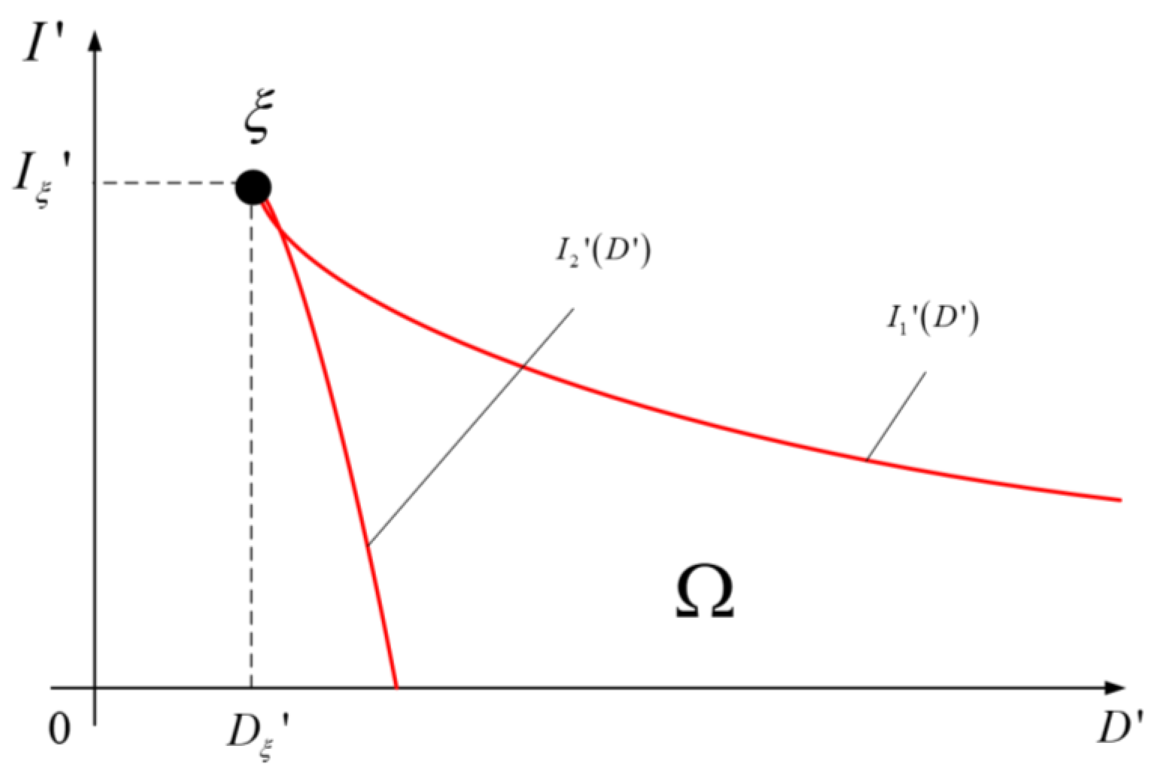
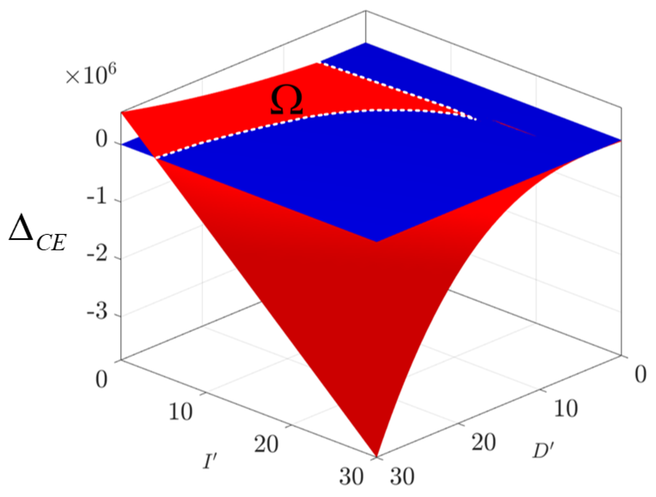
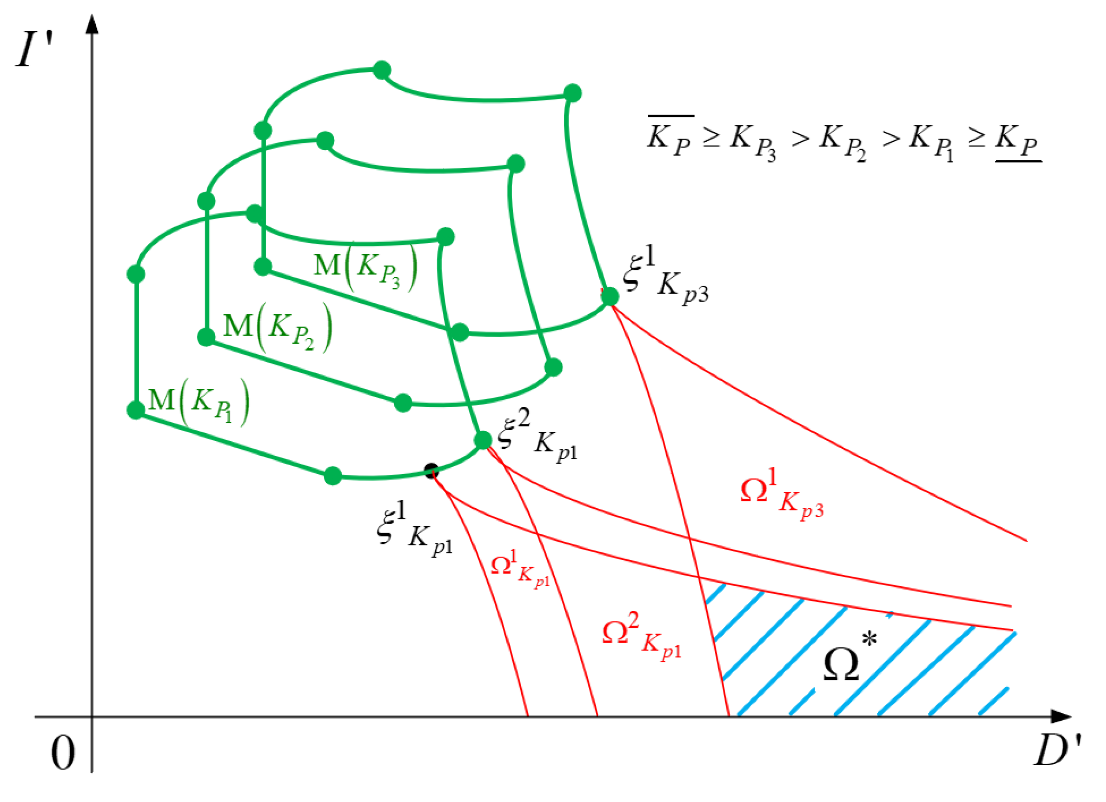
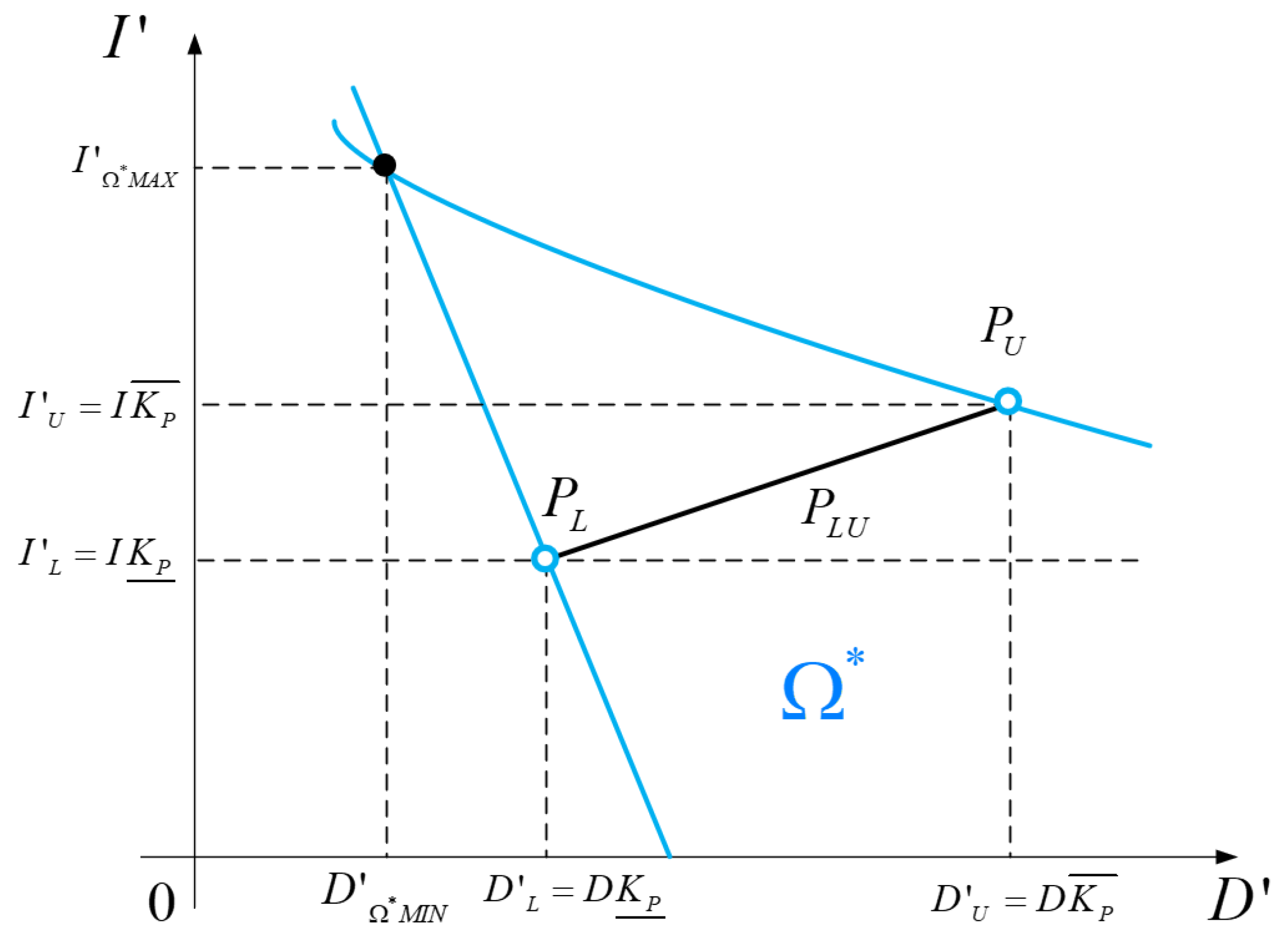
2.4. Constraints Clarification for ${\mathsf{\Omega }}^{*}$

The next problem in the research is to generalize constraints for ${\mathsf{\Omega }}^{*}$. It can be suggested that ${\mathsf{\Omega }}^{*}$ is constrained with (5) for arguments providing the ${I^{\prime }}_{\xi }$ value to be minimum according to (6) maximum ${D^{\prime }}_{I_0}$—the value of $D^{\prime }$ that turns ${I^{\prime }}_2(\alpha ,\omega ,k^{\prime },D^{\prime })$ into zero. The value of ${D^{\prime }}_{I_0}$ is defined as follows:

$${D^{\prime }}_{I_0}\left(\alpha ,\omega ,K^{\prime }\right)=-2\alpha +2\sqrt{\left({\alpha }^2+{\omega }^2+K^{\prime }\right)}.$$

(18)

It should be noted that desired points ${\xi }_1$ and ${\xi }_2$ can either belong to vertices or edges mapping of MIRL. For further convenience, (7) and (18) can be rewritten as functions of plant model parameters. Since (1) and (17) are equivalent representations of the plant transfer function, (7) and (18) can be represented as follows:

$${I^{\prime }}_{\xi }(a,b,c,K^{\prime })=\frac{\frac{1}{a^3}\sqrt{3{\left(4a^4+4K^{\prime }{a}^2+4ca-b^2\right)}^3}}{72},$$

(19)

$${D^{\prime }}_{I_0}\left(a,b,c,K^{\prime }\right)=2\sqrt{\frac{c}{a}+K^{\prime }}-\frac{b}{a}.$$

(20)

Regarding the assumption that desired points ${\xi }_1$ and ${\xi }_2$ belong to edges of MIRL mapping $M\left(K_{P_i}\right)$, it should be noted that the only possible way of edge location for ${\xi }_1$ and ${\xi }_2$ is a nonmonotonic behavior of (19) or (20). It is known that each edge of MIRL and, consequently, its mapping $\mathrm{M}\left(K_P\right)$ are formed by the varying of single interval parameters with others fixed in their limit values, and it turns (19) and (20) into one-variable functions forming each edge.

In order to define whether (19) and (20) are monotonic or not along each interval parameter, one can find partial derivatives for (19) and (20) with respect to $a$, $b$, $c$, and $K^{\prime }$ for checking their monotonicity property. Partial derivation for (19) yields:

$$\frac{\partial {I^{\prime }}_{\xi }(a,b,c,K^{\prime })}{\partial a}=\frac{\sqrt{3}\left(4a^4-2ca+b^2\right){\left(4a^4+4K^{\prime }{a}^2+4ca-b^2\right)}^2}{24a^4\sqrt{{\left(4a^4+4K^{\prime }{a}^2+4ca-b^2\right)}^3}}$$

(21)

$$\frac{\partial {I^{\prime }}_{\xi }(a,b,c,K^{\prime })}{\partial b}=-\frac{\sqrt{3}b{\left(4a^4+4K^{\prime }{a}^2+4ca-b^2\right)}^2}{24a^3\sqrt{{\left(4a^4+4K^{\prime }{a}^2+4ca-b^2\right)}^3}}$$

(22)

$$\frac{\partial {I^{\prime }}_{\xi }(a,b,c,K^{\prime })}{\partial c}=\frac{\sqrt{3}{\left(4a^4+4K^{\prime }{a}^2+4ca-b^2\right)}^2}{12a^2\sqrt{{\left(4a^4+4K\prime a^2+4ca-b^2\right)}^3}}$$

(23)

$$\frac{\partial {I^{\prime }}_{\xi }(a,b,c,K\prime )}{\partial c}=\frac{\sqrt{3}{\left(4a^4+4K^{\prime }{a}^2+4ca-b^2\right)}^2}{12a\sqrt{{\left(4a^4+4K^{\prime }{a}^2+4ca-b^2\right)}^3}}$$

(24)

Investigating (21)–(24), it can be concluded that if $4a^4+4K^{\prime }{a}^2+4ca-b^2$ and $4a^4-2ca+b^2$ possess a non-zero value at any $a\in \left[\underset{\_}{a},\overline{a}\right]$, $b\in \left[\underset{\_}{b},\overline{b}\right]$, $c\in \left[\underset{\_}{c},\overline{c}\right]$, and $K^{\prime }\in \left[\underset{\_}{K^{\prime }},\overline{K^{\prime }}\right]$, then (19) has a monotonic behavior. Alternatively, for solutions for one of (21), (22), (23), or (24) with respect to changing variables, one can get the exact investigated parameter value that gives ${\xi }_1$.

Similarly, partial derivation for (20) gives:

$$\frac{\partial {D^{\prime }}_{I_0}\left(a,b,c,K^{\prime }\right)}{\partial a}=\frac{b-\frac{c}{\sqrt{\frac{c}{a}+{K^{\prime }}^2}}}{a^2},$$

(25)

$$\frac{\partial {D^{\prime }}_{I_0}\left(a,b,c,K^{\prime }\right)}{\partial b}=-\frac{1}{a},$$

(26)

$$\frac{\partial {D^{\prime }}_{I_0}\left(a,b,c,K^{\prime }\right)}{\partial c}=\frac{1}{a\sqrt{\frac{c}{a}+{K^{\prime }}^2}},$$

(27)

$$\frac{\partial {D^{\prime }}_{I_0}\left(a,b,c,K^{\prime }\right)}{\partial K^{\prime }}=\frac{1}{\sqrt{\frac{c}{a}+K^{\prime }}}.$$

(28)

Functions (26)–(28) are always non-zero, so that it is sufficient to check the behavior of (25). In addition, one has to check (25) only in the case of parameter $a$ variation.

Regarding the aforementioned results, if (21)–(28) are monotonic functions within interval parameters bounds, in special points ${\xi }_1\left({\alpha }_L,{\omega }_L\right)$ and ${\xi }_2\left({\alpha }_U,{\omega }_U\right)$ that define regions in which intersection gives ${\mathsf{\Omega }}^{*}$, only two members of interval family form the set containing $I^{\prime }$ and $D^{\prime }$ values that satisfies non-overshoot conditions for all the interval family. The two special members of the family are defined as follows:

$$W_{\xi 1}\left(s\right)=\frac{\underset{\_}{K_P}}{\overline{a}{s}^2+\underset{\_}{b}s+\overline{c}},$$

(29)

$$W_{\xi 2}\left(s\right)=\frac{\overline{K_P}}{\underset{\_}{a}{s}^2+\underset{\_}{b}s+\overline{c}}.$$

(30)

In case some of (21)–(28) are non-monotonic, one has to find the exact solution with respect to varying parameters and substitute it to (29) or (30), instead of limiting the value of the parameter.

2.5. PID-Controller Coefficient Choice

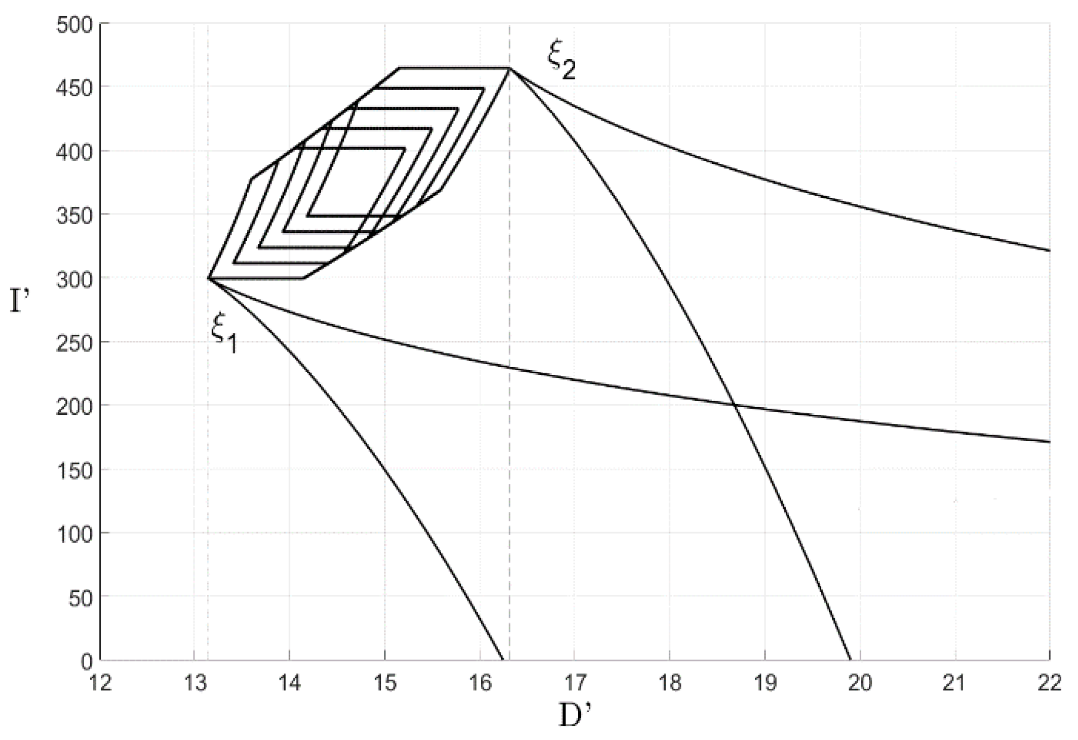
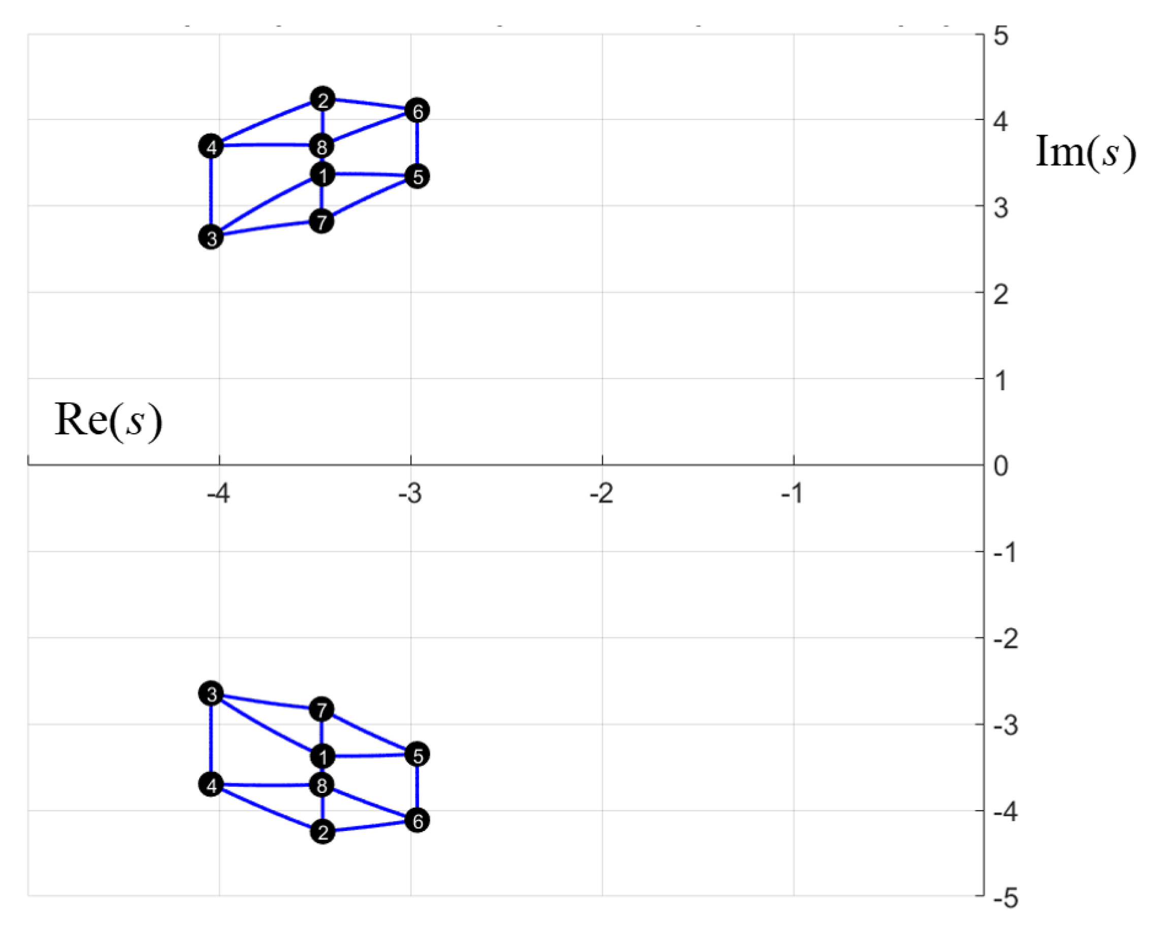
The final problem within the present research is to find the exact values for the PID-controller coefficients $D$ and $I$. One has to note that $D^{\prime }=K_{P}D$ and $I^{\prime }=K_{P}I$ are interval values, since $K_P$ is a given interval. Thus, it is essential to find $D$ and $I$ values such that:

$$\left\{D^{\prime }\in {\mathsf{\Omega }}^{*},I^{\prime }\in {\mathsf{\Omega }}^{*}|\forall K_P\in [\underset{\_}{K_P};\overline{K_P}]\right\}.$$

(31)

In order to satisfy (31), one can check two points denoted as $P_U\left(D\overline{K_P},I\overline{K_P}\right)$ and $P_L\left(D\underset{\_}{K_P},I\underset{\_}{K_P}\right)$, since any point $\left(D{K_P}^{*},I{K_P}^{*}\right),K_P\in [\underset{\_}{K_P};\overline{K_P}]$ belongs to the linear interval $P_{LU}$. Let us investigate the generalized condition for $P_{LU}$ to lay within the ${\mathsf{\Omega }}^{*}$ region. In other words, the following problem is to choose $D$ and $I$ in such a way that $P_{LU}\in {\mathsf{\Omega }}^{*}$ is as depicted in Figure 6.

According to Figure 6, one can observe that with a known range of gain $K_P$ and known expression for constraints (5), $D$ and $I$ values providing $P_{LU}\in {\mathsf{\Omega }}^{*}$ can be found from inequality of the form:

$$\frac{{I^{\prime }}_U\left({\alpha }_U,{\omega }_U,{K^{\prime }}_U,{D^{\prime }}_U\right)}{\overline{K_P}}\ge \frac{{I^{\prime }}_L\left({\alpha }_L,{\omega }_L,{K^{\prime }}_L,{D^{\prime }}_L\right)}{\underset{\_}{K_P}}$$

Regarding the limit case, i.e., $P_L\in {I_2}^{\prime }$ and $P_U\in {I_1}^{\prime }$, the aforementioned inequality can be represented as the following equality:

$$\frac{{I^{\prime }}_U\left({\alpha }_U,{\omega }_U,{K^{\prime }}_U,{D^{\prime }}_U\right)}{\overline{K_P}}=\frac{{I^{\prime }}_L\left({\alpha }_L,{\omega }_L,K_{\mathrm{L}}^{\prime },{D^{\prime }}_L\right)}{\underset{\_}{K_P}}.$$

(32)

3. Example

In order to verify the obtained results, let us consider arbitrary second-order transfer functions with interval-given parameters that are described with the expression:

$$W(s)=\frac{\left[16,18\right]}{\left[1.2,1.4\right]s^2+\left[8.3,9.7\right]s+\left[28,36\right]}$$

(33)

Using MATLAB, let us plot the MIRL of (33). The MIRL for (33) is shown in Figure 7.

Regarding the results obtained in [19], one can obtain the external border of the MIRL presented in Figure 7 by vertices numbered as $3,4,2,6,5,7$, and corresponding edges that connect external vertices. The candidate transfer functions according to (29) and (30) for the plant are:

$$W_{\xi 1}\left(s\right)=\frac{16}{1.4s^2+8.3s+36}$$

$$W_{\xi 1}\left(s\right)=\frac{18}{1.2s^2+8.3s+36}$$

The investigation according to (21)–(28) yields that candidate functions are satisfied in the aforementioned conditions and, thus, define ${\mathsf{\Omega }}^{*}$. $W_{\xi 1}$ and $W_{\xi 2}$ parameters are: ${\alpha }_L=3.4643$, ${\omega }_L=2.8282$, ${\alpha }_U=3.4526$, and ${\omega }_U=4.2461$. With respect to $W_{\xi 1}$ and $W_{\xi 2}$ as proportional coefficients for PID controllers, the lowest values should be chosen, and according to (14), one can obtain $K=6.5808$, and thus, $K^{\prime }=K{K}_P=\left[75.2091,98.712\right]$.

For the investigated plant, regarding the external border presented in Figure 7, mapping $M\left(K_P\right)$ for different $K_P$ values within its range was calculated and plotted (see Figure 8).

Substituting ${\alpha }_L=3.4643$, ${\omega }_L=2.8282$, ${\alpha }_U=3.4526$, and ${\omega }_U=4.2461$ into (5), one can obtain analytical expression for ${\mathsf{\Omega }}^{*}$ constraints and that gives:

$${I^{\prime }}_U\left(D^{\prime }\right)=32.2913D^{\prime }-\frac{2\sqrt{{\left({D^{\prime }}^2+13.8104D^{\prime }-338.3036\right)}^3}}{27}-1.54{D^{\prime }}^2-0.074{D^{\prime }}^3+271.756$$

$${I^{\prime }}_L\left(D^{\prime }\right)=21.0685D^{\prime }+\frac{2\sqrt{{\left({D^{\prime }}^2+13.8527D^{\prime }-237.6221\right)}^3}}{27}-1.53{D^{\prime }}^2-0.074{D^{\prime }}^3+195.251$$

Next, solving (32) with respect to variable $D^{\prime }$ yields $P_U\left(19.9695,90.8278\right)$ and $P_L\left(17.1167,77.8524\right)$, calculation of the PID-controller coefficients gives the following results: $D=1.331$, $K=6.5808$, and $I=6.055$. For the obtained values, the condition $P_{LU}\in {\mathsf{\Omega }}^{*}$ holds and provides a non-overshooting closed-loop step response for (2). The obtained closed-loop transfer function has the following form

$$W_{CL}(s)=\frac{\left[11.43;15\right]\left(1.331s^2+6.581s+6.055\right)}{s^3+\left[21.1379;28.049\right]s^2+\left[95.2234;128.712\right]s+[69.1985;90.8226]}$$

For confirmation results, let us obtain step responses for $W_{CL}(s)$ in different realizations, i.e., with different parameters value combinations. In Figure 9, fifty different members of the interval family are presented.

In Figure 9, there are a set of step responses for $W_{CL}(s)$ that are obtained with regular steps of each parameter combination, and the overshoot value is zero for each of the responses.

4. Conclusions

This paper presents the approach for PID-controller tuning providing a non-overshoot step response for a second-order transfer function with interval-given parameters. Designed for a stationary LTI-system approach based on necessary conditions of closed-loop poles, a real configuration with further application is necessary, and sufficient conditions within the region $\mathsf{\Omega }$ of PID-controller parameters guarantees strictly real closed-loop poles. Next, the rule for proportional coefficient calculation was introduced while holding necessary and sufficient conditions in every point that belong to region $\mathsf{\Omega }$. In addition, another key performance index in many control applications is the stability degree [29,30]. In this paper, (9) defines the maximum stability with respect to plant parameters and chosen proportional PID-controller coefficients and thus allows us to tune the PID controller according to desired stability degree.

Considering parametric uncertainty and its interval representation, the approach was enhanced and applied to this class of systems. Since in systems with interval-given parameters, poles move and form regions of localization, the approach has to regard a certain set of cases. Using (5) and (6), one can get mapping of poles’ localization regions into a PID-controller parameter plane. The next step was getting the region of PID-controller coefficients that allows maintaining the aforementioned conditions for each member of interval family. Finally, regarding all constraints and conditions, the equation whose solution gives the exact PID-controller coefficient was formulated.

One of the key disadvantages is difficulty of enhancing of the presented results for higher-order systems due to lack of analytical methods for a higher-order equation solution. Using the Ferrari method for a fourth-order equation, plant model objects can probably be third-order. On the other hand, a wide class of typical industrial plants can be described with second- or third-order transfer function [31] that makes the presented approach applicable for many problems.

One of the main advantages of the approach is a high degree of generality, since all basic functions and expression are presented in general form, and one can investigate how exactly the parameters of the controller or plant affect the design procedure and, thus, the final result. The generalization of design techniques allows us to eliminate so-called “loss of insight”, in which [32] corresponded to a numerical calculation. As a direction of further research, generalizing results for transfer functions of higher order with zeros should be examined. Another topic of further research can be PID-controller design with consideration of settling time, energy, and more complex kinds of uncertainties as well. Moreover, regarding future directions of research, one thought is to enhance it to linear time-varying (LTV) systems, since despite being in the class of LTV systems, its parameters are not just regular intervals, but functions of time. Due to fundamental physical constraints, ranges of definition for such kind of functions are constrained as well. The presented research forms the minimal necessary basis for providing a required performance index within the given interval, and the possible next step is to advance control quality with respect to law of parameters variation and other conditions [33].

References

1. Moore, K.L.; Bhattacharyya, S.P. A technique for choosing zero locations for minimal overshoot. IEEE Trans. Autom. Control 1990, 35, 577–580. [Google Scholar] [CrossRef]
2. Efimov, S.V.; Kurgankin, V.V.; Zamyatin, S.V. Designing transfer function with the required direct performance measures based on the Laplace transform. Optoelectron. Instrum. Data Process. 2014, 50, 348–353. [Google Scholar] [CrossRef]
3. Hauksdottir, A.S. A sufficient and necessary condition for extrema-free step responses of single-zero continuous-time systems with real poles. In Proceedings of the 38 Conference on Decision & Control, Phoenix, AZ, USA, 7–10 December 1999; pp. 499–500. [Google Scholar]
4. Hauksdottir, A.S. Analytic Expression of Transfer Function Reponses and Choice Numerator Coefficients (Zeros). IEEE Trans. Autom. Control 1996, 41, 1482–1488. [Google Scholar] [CrossRef]
5. Hauksdottir, A.S.; Hjaltadottir, H. Closed-form expressions of transfer function responses. In Proceedings of the American Control Conference, Denver, CO, USA, 4–6 June 2003; pp. 3234–3239. [Google Scholar]
6. Herjolfsson, G.; Hauksdottir, A.S. Direct computation of optimal PID controllers. In Proceedings of the 42nd IEEE Conference on Decision and Control, Maui, HI, USA, 9–12 December 2003; pp. 1120–1225. [Google Scholar]
7. Jayasuriya, S.; Dharne, A.G. Necessary and sufficient conditions for non-overshooting step responses for LTI systems. In Proceedings of the 2002 American Control Conference, Anchorage, AK, USA, 8–10 May 2002; pp. 500–510. [Google Scholar]
8. Nguyen, N.H.; Nguyen, P.D. Overshoot and settling time assignment with PID for first-order and second-order systems. IET Control Theory Appl. 2018, 12, 2407–2416. [Google Scholar] [CrossRef]
9. Prakash, R.; Anburaja, S.A.; Rishivanth, S.; Govinda Kumar, E. Non-overshoot time response of third order system using cascade PID-Lead compensator controller. In Proceedings of the 2017 Second International Conference on Electrical, Computer and Communication Technologies (ICECCT), Coimbatore, Tamil Nadu, India, 22–24 February 2017; pp. 1–6. [Google Scholar]
10. Visioli, A. Practical PID Control, 1st ed.; Springer: London, UK, 2006; p. 314. [Google Scholar]
11. Anbarasan, M.; Suji Prasad, S.J.; Meenakumari, R.; Balakrishnan, P.A. Modified PID controller for avoiding overshoot in temperature of barrel heating system. In Proceedings of the 2013 International Conference on Emerging Trends in VLSI, Embedded System, Nano Electronics and Telecommunication System (ICEVENT), Tiruvannamalai, Tamil Nadu, India, 7–9 January 2013; pp. 1–6. [Google Scholar]
12. Souza, M.R.S.B.; Murofushi, R.H.; Tavares, J.J.P.Z.; Ribeiro, J.F. PID Tuning for the Pitch Angle of a Two-Wheeled Vehicle. In Proceedings of the 2015 12th Latin American Robotics Symposium and 2015 3rd Brazilian Symposium on Robotics (LARS-SBR), Uberlândia, Brazil, 28 October–1 November 2015; pp. 371–375. [Google Scholar]
13. Wu, H.; Su, W.; Liu, Z. PID controllers: Design and tuning methods. In Proceedings of the 2014 9th IEEE Conference on Industrial Electronics and Applications (ICIEA), Hangzhou, China, 9–11 June 2014; pp. 808–813. [Google Scholar]
14. Kobayashi, H. Output overshoot and pole-zero configuration. In Proceedings of the 12th IFAC World Congress Automat. Contr., IFAC, Sydney, Australia, 18–23 July 1993; pp. 529–532. [Google Scholar]
15. Lin, S.K.; Fang, C.J. Nonovershooting and monotone nondecreasing step responses of a third-order SISO linear system. IEEE Trans. Autom. Control 1997, 42, 1299–1303. [Google Scholar]
16. Zhmud, V.; Yadrishnikov, O.; Poloshchuk, A.; Zavorin, A.A. Modern key technologies in automatics: Structures and numerical optimization of regulators. In Proceedings of the 2012 7th International Forum on Strategic Technology (IFOST), Tomsk, Russia, 18–21 September 2012. [Google Scholar]
17. Prokopiev, A.P.; Ivanchura, V.I.; Emelyanov, R.T. Synthesis PID Controller for Objects Second Order with Regard to the Location Poles. J. Sib. Fed. Univ. Eng. Technol. 2016, 1, 50–60. [Google Scholar] [CrossRef]
18. Nesenchuk, A.A. A method for synthesis of robust interval polynomials using the extended root locus. In Proceedings of the 2017 American Control Conference (ACC), Seattle, WA, USA, 24–26 May 2017; pp. 1715–1720. [Google Scholar]
19. Sukhodoev, M.S.; Gayvoronskiy, S.A.; Zamyatin, S.V. Parametric synthesis of linear regulator in interval system with guaranteed root quality indices. Bull. Tomsk Polytech. Univ. 2007, 311, 9–12. [Google Scholar]
20. Ouyang, H.; Yue, J.; Su, Y. Design and Application of PID Controllers Based on Interval Computing Theory. In Proceedings of the 2011 International Conference on Electrical and Control Engineering, Yichang, China, 16–18 September 2011; pp. 1505–1510. [Google Scholar]
21. Chapellat, H.; Bhattacharyya, S.P. A generalization of Kharitonov’s theorem; Robust stability of interval plants. IEEE Trans. Autom. Control 1989, 34, 306–311. [Google Scholar] [CrossRef]
22. Zhmud, V.; Zavorin, A. The design of the control system for object with delay and interval-given parameters. In Proceedings of the 2015 International Siberian Conference on Control and Communications (SIBCON), Omsk, Russia, 21–23 May 2015. [Google Scholar]
23. Marcillo, K.E.L.; Guingla, D.A.P.; Barra, W.; De Medeiros, R.L.P.; Rocha, E.M.; Benavides, D.A.V.; Nogueira, F.G. Interval robust controller to minimize oscillations effects caused by constant power load in a DC multi-converter buck-buck system. IEEE Access 2019, 7, 26324–26342. [Google Scholar] [CrossRef]
24. Marcillo, K.E.L.; Rocha, E.M.; Junior, W.B.; Benavides, D.A.V.; de Medeiros, R.L.P.; Alves, M.S.; Leão, M.P.V. Robust control for DC–DC buck converter under parametric uncertainties. In Proceedings of the 22nd Congresso Brasileiro de Automatica (CBA), Paraiba, Brazil, 9–12 September 2018; pp. 1–8. [Google Scholar]
25. Tsavnin, A.V.; Efimov, S.V.; Zamyatin, S.V. Providing real closed-loop transfer functions poles for plant with interval-given parameters for overshoot elimination. In Proceedings of the 11th International Congress on Ultra Modern Telecommunications and Control Systems and Workshops (ICUMT), Dublin, Ireland, 28–30 October 2019; pp. 1–7. [Google Scholar]
26. Andrakhanov, A.; Belyaev, A. Navigation learning system for mobile robot in heterogeneous environment: Inductive modeling approach. In Proceedings of the 12th International Scientific and Technical Conference on Computer Sciences and Information Technologies (CSIT 2017), Lviv, Ukraine, 5–8 September 2017; pp. 543–548. [Google Scholar]
27. Andrakhanov, A.; Belyaev, A. GMDH-Based Learning System for Mobile Robot Navigation in Heterogeneous Environment. In Advances in Intelligent Systems and Computing; Shakhovska, N., Stepashko, V., Eds.; Springer: Cham, Switzerland, 2018; Volume 689, pp. 1–20. [Google Scholar]
28. Fadeev, A.S.; Zarnitsyn, A.Y.; Tsavnin, A.V.; Belyaev, A.S. Cyber-physical system prototype development for control of mobile robots group for general mission accomplishment. In Proceedings of the Second International Conference on Material Science, Smart Structures and Applications: ICMSS-2019, Erode, India, 21–22 November 2019. [Google Scholar]
29. Pushkarev, M.I.; Gaivoronsky, S.A.; Efimov, S.V.; Zamyatin, S.V. Parametric synthesis of maximum stability degree and specified accuracy linear automatic control system PI-controller. In Proceedings of the 18th International Conference on Soft Computing, MENDEL 2012, Brno, Czech Republic, 27–29 June 2012; pp. 344–349. [Google Scholar]
30. Pushkarev, M.I.; Efimov, S.V.; Gayvoronsky, S.A.; Chenkova, O.A. A single-loop DC motor control system design with a desired aperiodic degree of stability. In Proceedings of the International Conference on Mechanical Engineering, Automation and Control Systems 2015 MEACS 2015, Tomsk Polytechnic University, Tomsk, Russian, 1–4 December 2015. [Google Scholar]
31. Astrom, K.J.; Hagllund, T. PID Controllers Theory, Design and Tuning, 2nd ed.; Instrument Society of America: Pittsburgh, PA, USA, 1994. [Google Scholar]
32. Barmish, B.R. New Tool for Robustness of Linear Systems; Macmillan Publishing Company: New York, NY, USA, 1994. [Google Scholar]
33. Xiang, W.; Xiao, J. Stabilization of switched continuous-time systems with all modes unstable via dwell time switching. Automatica 2014, 3, 940–945. [Google Scholar] [CrossRef]
Figure 1. Typical closed-loop structure.
Symmetry 12 01092 g001
Figure 2. Surface of discriminant values with zero plane.
Symmetry 12 01092 g002
Figure 3. Region Ω in a plane of controller coefficients D I .
Symmetry 12 01092 g003
Figure 4. Multiparametric interval root locus for second-order plant with parametric uncertainties.
Symmetry 12 01092 g004
Figure 5. Set of mappings M ( K P i ) of multiparametric interval root locus (MIRL) with respect to the K P range.
Symmetry 12 01092 g005
Figure 6. P L and P U localization within Ω * and corresponding D and I ranges.
Symmetry 12 01092 g006
Figure 7. Interval root locus for (33).
Symmetry 12 01092 g007
Figure 8. Set of experimental mappings M ( K P i ) of the MIRL external border for (33) and obtained ξ 1 and ξ 2 .
Symmetry 12 01092 g008
Figure 9. Experimental set of step responses for obtained closed-loop transfer function.
Symmetry 12 01092 g009