Abstract
As it is well acknowledged that the electoral system is one of the fundamental rocks of our modern society, the behavior of electors engaged in a voting system is of the utmost importance. In this context, the goal of the study is to model the behavior of voters in a first-past-the-post system and to analyze its consequences on a party system. Among the assumptions of this study is Duverger’s law, which states that first-past-the-post systems favor a two-party system as the voters engage in tactical voting, choosing to vote in favor of a less preferred candidate who has better odds of winning. In order to test this assumption and to better analyze the occurrence of the strategic behavior, a laboratory experiment was created. A total of 120 persons participated in the study. An asymmetrical payoff function was created to value the voters’ preference intensity. As a result, it was observed that as voters got used to the voting system, they engaged in more tactical voting behavior in order to either maximize the gain or minimize the loss of their choice. Moreover, the iterations where voters started displaying tactical behavior featured a clustering around two main choices. The obtained results are consistent with both the empirical results of real-life elections and Duverger’s law. A further discussion regarding the change in voters’ choice completes the analysis on the strategic behavior.
1. Introduction
The electoral system plays an important role in modern democratic society, with an impact on the future of the societies we live in. A proper voting system ensures the very democracy of our modern world, offering necessary and meaningful change and an effective system of “governance”.
Several studies have been written in the field, each of them addressing different aspects related to the electoral system, such as electoral disproportionality [], electoral system comparison [], influencing voters’ choice [], election planning and election scenarios [,], e-voting and voting accounts [,,,], voting behavior [], youth participation [] and examination of the accuracy of forecasting methods [].
In the present paper the focus is on first-past-the-post electoral systems, as these systems are widely used worldwide for various types of elections, such as presidential elections and legislative elections. For parliamentary elections under a first-past-the-post system, elections are comprised of multiple local elections, each deciding the local representative for a seat in parliament.
This system is used in many countries, including countries with large populations, around the world. First-past-the-post systems are used in two of the most populous democratic states (the United States of America and India) and in states with long and entrenched democratic traditions.
Because of the importance of these systems, it is necessary to understand the way they work. Under the assumption of multiple parties which nominate candidates, legislative elections under a first-past-the-post system may lead to nationwide results which are not proportional with the number of votes received by each party.
First-past-the-post elections result in the election of one person from a pool of one or more candidates. This can happen over one or more rounds, the winner being the person who gets the most votes in the last round of the process.
Regarding the scientific literature, several papers have discussed issues related to the effects of different electoral rules on the electoral system, as tested by Lijphart [], Cox [] and Norris []. Endersby and Shaw [] undertook experiments and simulations in order to evaluate the effect of first-past-the-post electoral systems. As for Duverger’s Law, Rich [] considered how institutional factors shape district competition in mixed legislative systems, whereas Clark and Golder [] unpacked the competing mechanisms that Duverger proposed. Other researchers such as Chhibber and Kollman [] sought to understand how the effectiveness of Duverger’s law is dependent on the powers the government has. Fujiwara [] used other causal identification approaches for evaluating the law’s effect. A series of substantial works discussing tactical voting under first-past-the-post systems can be found [,,,,,,]. Considering the scientific literature, it can be seen that most of the studies have focused on analyzing how the first-past-the-post election mechanism has affected the results of elections, and on identifying the underlying causes that led to such results [,,,,,], whereas only few studies have focused on laboratory experiments [,]. While considering the studies featuring laboratory experiments, it can be observed that in most of the studies, two voting parties were taken into account [,,], and the provided information was either complete or incomplete. In most of the cases, each participant in the experiment possessed knowledge related to his/her own preferences and costs related to the voting options, without knowing any additional information related to other participants’ preferences and voting costs [,,]. As a result, during the voting process, the participants received symmetrical information, although all the participants had, in fact, asymmetrical information about the voting process as a whole.
This study will only discuss first-past-the-post elections with one round and more than one candidate. The scope of this analysis is to see whether this voting system can be considered suitable and sustainable from a democratic point of view, or whether it can be biased by the fact that voters can gather additional information. The source of the additional information can vary, from statistics made available before voting on different communication media (such as television or social media) to the knowledge accumulated by the voters’ participation in past voting processes. Nevertheless, as in most of the cases in which the first-past-the-post system is used, a lack of proportionality has been observed. The paper aims to understand the underlying micro-processes which contribute to the macro-result. As previously stated in the literature [], in the first-past-the-post system the voter should first determine the odds that his/her preferred party will win the elections and, based on this prediction, he/she can engage in tactical voting. Nevertheless, as Blais et al. [] showed, there are cases in which the tactical behavior is hard to be seen at equilibrium, as some of the voters can engage in mixed strategies based on access to new information.
The main working hypothesis of the study is Duverger’s Law, which states that first-past-the-post systems with one round of voting favor the biggest two parties, thus leading to a two-party system []. Through the analysis of first-past-the-post systems in different countries, it will be demonstrated that the system leads to an overrepresentation of the largest two parties. Even more, it will be shown that this overrepresentation is the result of the system itself, not conditions particular to each election.
As for the micro-behavior, an experiment is conducted using 120 participants in order to provide a quantitative and experimental basis to Duverger’s law, which will be used to further analyze how the voters engage into tactical voting.
Unlike other laboratory experiment-based studies from the field, which focused on the rational consideration of the result (see [,,,,,]) and which did not use any of the words related to a voting system (e.g., “election”, “vote”, “parties”, etc.) [], this study properly informs the participants regarding the fact that they are going to take part in a “simulated” voting process, similar to the ones used in elections. This decision is in line with the suggestions made by Blais et al. []. Moreover, the utility function has been built upon, using different payoff values in order to better shape the intensity of preferences, as suggested by Cooter []. This approach differs from other laboratory experiments as it puts the participants in a more “conscious” situation by offering them information related to the study and by informing them of the results of each election round. The results are analyzed on each panel of participants based on the expected and obtained utilities.
The paper is organized as follows: Section 2 presents how first-past-the-post systems work in different countries around the world, while describing both the historical evolution of the system and the way legislative mandates were distributed in some countries. Section 3 analyzes how the system actually works and proves that the system will produce distortions in the seat/vote curve even without voters engaging in tactical voting, while Section 4 provides a laboratory experiment approach in order to test for the presence of tactical voting among voters. In order to account for each person’s intensity of preference regarding a political party, an asymmetrical payoff function was built. Section 5 analyzes the voters’ strategic behavior, and in Section 6 the main conclusions of the study are highlighted. The instruments used in the laboratory experiment are provided in the Appendices.
2. The First-Past-the-Post System in the World
The first-past-the-post system is commonly used in different states all over the world, such as the United Kingdom, the United States of America, Canada and India. Even though referendums have been held over time in order to see whether this voting system should be changed (e.g., the UK’s electoral reform referendum of May 2011 []), the referendum proposals have been defeated and the first-past-the-post system continues to be used. In the following section, an overview of the adoption of the first-past-the-post system in two of the above-mentioned countries is presented along with some results from the electoral voting processes.
2.1. The First-Past-the-Post System in the United Kingdom
In England, the parliament was at first a council of the king, which gained more and more power over time. Parliamentary representation had a territorial basis. There were two types of divisions: “counties” based on rural areas, and “boroughs” for cities and towns. Each constituency was represented by two members of parliament []. Representation on a geographical basis is consistent with the fact that the medieval economy was based on land. Moreover, the electoral system was simple: the candidate with the largest number of votes was the one elected [].
We can notice that the main characteristics of the first-past-the-post system were already in use: the territory of the state was divided into territorial constituencies, each one of them organizing a separate electoral competition in order to elect its own representatives. The candidates with the largest number of votes were elected. These elections differed from first-past-the-post elections only by the fact that constituencies had two representatives rather than one.
The British system evolved to become a first-past-the-post system partially due to the inherited territorial characteristics of the political system. This fact may show that the first-past-the-post systems have a better capacity of representing local interests.
After the Second World War, British politics were dominated by two big parties, namely the Conservative Party and the Labor Party. During the second half of the 20th century, only the February 1974 elections did not result in a majority for one party []. In this period, a growth in the number of votes for the third party did not result in a corresponding number of parliamentary mandates for that party [].
In the 1990s and early 2000s, British elections continued to result in majorities for one party, while the percentages for a third party continued to be significant. As a result, the third party had over 10% in all elections after 1974 and over 20% in 1983, 1987 and 2005 [].
The last British elections took place in 2017 and were won by the Conservative Party with a small vote margin []. According to the result published by BBC, the most overrepresented parties of these elections were the Labor Party and the Scottish National Party [].
As Table 1 shows, the Scottish National Party was overrepresented along with the Conservative Party and, marginally, the Labor Party. This fact shows that in some cases not only the largest party is advantaged by the system, but also parties whose voters are highly concentrated in certain constituencies. That means that the distribution of voters among constituencies is also important in determining the way a legislative chamber will look after elections under a first-past-the-post system.

Table 1.
The results of the 2017 United Kingdom elections.
One should also note that the Scottish National Party only competes in Scotland, so its nationwide results are determined only by its results in Scotland (Table 2).
Table 2.
The results of the 2017 United Kingdom elections in Scotland.
The observation that the first-past-the-post system gives an advantage to the largest party can be seen in Table 2. The Scottish National Party managed to obtain nearly 60% of the Scottish seats in the United Kingdom parliament while having less than 40% of the vote share of the population in the area. As a result, it can be mentioned that the advantages of the first-past-the-post system, in this case, were translated into overrepresentation of the Scottish National Party, which might be due to the fact that the votes were concentrated in a distinct geographical area.
Due to problems that may arise from modelling such situations, in the present paper we will only take into account cases in which all parties have a national rather than a local presence.
2.2. The First-Past-the-Post System in the USA
The United States of America has a long tradition with the first-past-the-post system. In addition to having the first-past-the-post system, the United States has a political system dominated by two main parties, the Democratic Party and the Republican Party.
The power to decide the voting system is given to each state. Initially, most states adopted a system of multiple seat-constituencies in which the party with the most votes took all the seats in that constituency. Most states discontinued that system before 1840 in favor of a one seat per constituency first-past-the-post system []. One of the reasons for switching to a one seat per constituency system was to increase the proportionality of the results, because the old system led to disproportional results. Multiple seat constituencies were forbidden at the federal level in 1967 [].
The United States Congress is bicameral. The lower chamber has 435 members elected for two years. The upper chamber, called the Senate, was elected by state legislative chambers until 1913 []. Nowadays, senators are directly elected in each state. Every two years, a third of the senate is elected for a 6-year mandate [].
The United States Constitution specifies that each state will have two senators []. This allocation does not take into account the differences between state populations. This, along with the fact that senators are not elected at the same time, generates a first-past-the-post system with unequal constituencies.
This arrangement shows that a state’s option for a certain electoral system can have other considerations than assuring a more proportional national result. The choice to give each state an equal number of senators is rooted in the political conditions of the early United States.
Despite the fact that the American political system is dominated by two big parties, there can be significant disproportionalities between the number of a party’s mandates and its share of the popular vote []—see also Table 3.
Table 3.
The results of 8 elections of the House of Representatives of the Congress of the United States of America.
Table 3 shows that the biggest party tends to be overrepresented in the legislature under first-past-the-post voting even when there are just two parties.
However, the dominance of two big parties in the United Kingdom and the two-party system in the United States of America are not absolute proofs of the fact that first-past-the-post voting leads to a two-party system.
Apart from the first-past-the-post system, there are other reasons which led to the existence of the American two-party system. One of these reasons is that some states raised legislative barriers which make it harder for other parties to participate in electoral contests []. The two big parties—the Democrats and the Republicans—are the only ones with unrestricted access to participation in elections in all states, with other parties having to respect other conditions such as gathering signatures in order to participate in elections [].
In the following sections we will use two different approaches in order to compare the way the first-past-the-post system behaves. We will use simulation to study the way the first-past-the-post system works nationally and an experiment in order to explore the way voters behave in a constituency. A series of elements belonging to consumer economics and utility functions have been used in accordance with the economic literature dedicated to this area [,,,].
3. Macrolevel Implications of the First-Past-the-Post System
3.1. Assumptions
In order to simulate the distribution of seats in a first-past-the-post nationwide context it is necessary to determine a way of splitting the national votes into constituency votes.
As a result, for the simulation, strings of generated random numbers are needed, so that votes for each party are randomly distributed between constituencies. A string of random numbers, equal in length with the number of constituencies, will be generated for each party. As parties cannot have a negative number of votes, the strings were modified so that they had only positive numbers using the following equation:
where yi is the i-th element of the string formed after using the equation; xi is the i-th element of the original string.
After using the above equations, the resulting string of numbers lies between zero and one. Because in the next step each constituency result will be multiplied with the national result of one party, an additional sum for each string is necessary. The following equation is used:
where zi is the i-th of the string formed after using the equation, yi is the i-th element of the string formed after using the first equation and n is the total number of constituencies.
Based on these transformations, the following matrix with n lines and m columns (m being the number of parties) is obtained:
The constituency matrix, C, is obtained by multiplying each column with the national score of the party it corresponds to:
As first-past-the-post elections result in just one winner per constituency, for each line of the matrix, the largest number is replaced by one (signifying the winning party), whereas the others are replaced by zero. Then, by summing up each column, one can get the number of seats won by each party. As the simulation is based on strings of numbers, an additional analysis should be done in order to determine which distribution is more appropriate to the considered analysis.
The data regarding the number of votes for the top three parties in the 1923, 1924 and 1929 United Kingdom elections was used, as presented in Table 4 [].
Table 4.
Number of votes won by various parties during the 1923, 1924 and 1929 British elections.
The number of seats won by each party in the elections in the considered period are presented in Table 5.
Table 5.
Number of seats won by first three parties during the 1923, 1924 and 1929 British elections.
After a series of preliminary tests, it was found that T (Student) and χ2 distributions do not yield realistic results and they were removed from further testing. Table 6 provides the results of testing the different distributions. The algorithm was run 10,000 times and an average result was considered.
Table 6.
The results of the algorithm for the 1923, 1924 and 1929 British elections using 3 random distributions.
In order to establish which distribution yields the best results an error value was calculated. The value for the error is determined by subtracting the values obtained from the simulation results from the real ones, then the obtained result is squared. This process is carried out for each of the parties. When all the values have been computed, the results are summed up and divided by the number of the parties. Last, the square root is extracted.
The obtained results are presented in Table 7. As can be observed, in two of the three cases, the smallest error was generated by the uniform distribution, whereas in the third case, the exponential distribution generated the smallest error. As the exponential distribution generated the largest error in two other cases, the uniform distribution was chosen for the simulations.
Table 7.
The error associated with each distribution.
3.2. Parlamentary Mandates Simulation
A total of 10,000 runs were made using the uniform distribution. In all the runs, 1000 seats were considered, wanted by five parties. The national scores of each party were randomly generated using a normal distribution.
After generating scores for each simulation, they were ordered in descending order so that the results would be comparable.
Table 8 shows that the party with the highest scores (or number of votes) is overrepresented while the second largest party is proportionally represented. The last three parties are all underrepresented.
Table 8.
Average scores, number of seats and error of representation for each of the five simulated parties.
By analyzing all 10,000 runs, it was found that the difference in scores between the first and the second party was correlated with the number of seats of the first party, having a Pearson coefficient of 0.9353, whereas the correlation between this difference and the number of seats of the second party was −0.7995.
In addition, the number of seats of the first party was correlated with the number of seats it received, with a coefficient of 0.9355, whereas for the second party the correlation between its number of seats and its score was 0.9321.
For the first two parties a partial correlation between the difference of their scores and the number of seats they received was calculated. The results were: 0.57 for the first party and −0.60 for the second. Furthermore, the partial correlation between the number of seats received by each party and its score (excluding the difference of scores between the two parties) was 0.57 for the first party and 0.87 for the second.
For the first two parties, it was observed that their own number of votes remains the main predictor for the number of seats they received during the simulation. The difference in electoral scores between them also played a significant role in determining their number of seats.
In Figure 1 the number of seats won by the largest party has been represented using a red line, whereas the green area/line shows the initial score. It can be observed that the red line is above the green one in almost all cases, which signifies the fact that the most voted party was overrepresented constantly in the 10,000 simulations.
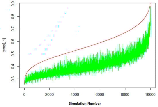
Figure 1.
The evolution of the number of seats (red line) based on the initial score (green line) for the largest party.
The significant variation of the green line for two close percentages of seats won shows that there are other explanatory variables beyond the initial number of votes received. The first and last parts of the graph have a more abrupt growth of the red line than the median part of it.
As for the other parties, it can easily be seen that the position of the red line keeps descending in relation with the position of the green one (Figure 2).

Figure 2.
The evolution of the number of seats (red line) based on the initial score (green line) of the last 4 parties.
In particular, for the second party, the red line is either under or over the green one. As can be observed in Figure 2, the red line begins under the green one which means that at a very low score the second party is underrepresented. Then, the red and green lines are at approximately the same level, meaning that for most of the graph the score of the second party corresponds with the number of seats it received. In the last part of the graph, the red line is over the green one, underlying the fact that when it received more votes, the second party was overrepresented. The abrupt growth of the line may also be caused by the influence the difference between the two biggest parties has on predicting their number of seats.
As for the last three parties, the green line is above the red one—see Figure 2. Considering the third party, the red line is most of the time under the green one and only in the last part of the graph does the red line go briefly above the red one. Thus, the third party is underrepresented most of the time. Therefore, it can be concluded that the only parties which have some advantages under the first-past-the-post system are the first and the second parties.
In the case of the fourth party, the red line is always under the green one, showing the fact that this party is underrepresented in all simulations. The number of seats gained grows quickly in the last section of the graph, which suggests that the efficiency of a percentage point (measured in seats gained for it) grew when the party had more votes.
Last, for the fifth party, the red line is superimposed on the x-axis of the figure, so it had zero seats in many of the trials. The green line sometimes “touches” the x-axis of the graph suggesting that in some trials the fifth party received zero votes by the random number generator. Even in the last part of the graph, where the red line grows quickly, its value is below the green one.
3.3. Discussions
The results of the simulations suggest that a first-past-the-post system favors the party with the greatest share of the vote and disadvantages the parties with fewer votes than the second most voted party. This conclusion is supported by the empirical facts presented above about real first-past-the-post elections.
Based on the simulation, it has been observed that the second party received a very slight advantage from the system and only in some rarer cases was it disadvantaged.
The simulation had some limitations. One of them is not taking into account the effects of tactical voting and other distorting factors that can favor a second-place party.
Nevertheless, the main conclusions yielded by the model can be considered valid. The simulation shows that even in the case of a random simulation, the first-past-the-post system continues to favor the biggest parties. Taking into account the results of the previous experiment, the fact that the biggest party is favored by the system may lead to a situation in which voters of the opposition concentrate around a single alternative party, thus leading to a two-party system.
However, the fact that the simulation did not take into account tactical voting may suggest that first-past-the-post systems favor larger parties even in the absence of tactical voting to reinforce this tendency.
Moreover, the fact that the second party may attract voters of other parties and thus grow stronger may also lead voters who are ideologically closer to the largest party to vote for it instead of their first choice in order to deny the opposition a win, thus reinforcing the two-party system even more.
The parties having fewer votes were constantly underrepresented in the simulations. This underrepresentation may make them lose voters to larger parties.
In conclusion, the simulation shows that even under a uniform distribution of votes on the territory of a country, a first-past-the-post system leads to results favoring the largest parties and thus the formation of two-party systems. Therefore, first-past-the-post systems lead to disproportionate results through themselves, not due to other factors. In other words, it can be stated that the system will produce distortions in the seat/vote curve even without tactical voting.
In order to have more conclusive results, other statistical distributions of results or an empirical distribution of votes per constituencies based on real results from real life elections can be further investigated.
4. Methodology for Analyzing the Microlevel Behavior of Voters
4.1. Assumptions
In order to explain first-past-the-post systems’ tendency to create two-party systems, it is also necessary to understand how voters behave when they participate in this kind of election. We developed an experiment which will offer some insight into how voters behave and how they adapt their behavior based on past results.
The main goal of the experiment is to determine if first-past-the-post systems lead to a concentration of votes towards two parties and, if such a concentration can be observed, how long it takes for it to manifest.
Considering the scientific literature, a series of general assumptions to be considered in the experiment emerge. On the one hand, we suppose that all parties are represented nationally. A second assumption is that parties to which the experiment is referring represent ideological positions, not groups of interests. A last assumption, derived from the previous assumptions, is that no party in the simulation has a particularly large local support.
On a micro level, five other assumptions emerge, presented as follows:
The first assumption is that each preference (or ideological position) has an equal number of people who consider it as their first choice. This assumption, although not realistic, is necessary due to the small sample size and the requirement of having at least two subjects with the same preferences in order to analyze their behavior.
Another assumption is that the vote is based solely on ideological preferences and that there are no other exogenous factors that shape individual preferences.
A third assumption is that ideological preferences form a spectrum, with each voter picking candidates that are closer to their own ideology.
A fourth assumption is that each subject participating in the experiment has static ideological preferences throughout all iterations. The purpose of this assumption is to control for ideological changes in the voting population in order to isolate the study to the influence of tactical voting.
A fifth assumption is that voters know the result of the previous iteration before deciding their option for the current one. Thus, after each iteration, voters were informed about the winning party and how many points they earned. If the number of votes for the first two options were equal, participants were given adjusted results: the votes for the option which won the most iterations up to that point were reduced by one vote, which was reallocated randomly.
The methodology used in constructing the experiment is based, as shown in the introduction, on the laboratory studies made in the scientific literature [,,] and on the theory of decision and choice (including the rules for building up a utility function) [,,,]. A noticeable difference between the present study and other laboratory experiments in the election field is the use of multiple parties in order to better observe the voting process and the occurrence of tactical voting. Considering, for example, the study made by Blais et al. [], several elements from the present study are similar. In that study, the voters’ utility was calculated based on how far the participants’ choices were from the party that received the most votes and the pay matrix was different for different participants, and each participant was aware only of his/her utility points, not knowing the voting preference of any of the other participants, nor the utility values of their cards. Among the differences is the fact that our participants started from an equal point at the beginning of each simulation (knowing their utility values and the result of the overall voting process), whereas in Blais et al. [] a hierarchy was randomly made at the start of each round. Another difference results from the fact that the participants did not receive a formula for determining their utility, but rather they had on their cards the values of their utility matrix in every iteration of the experiment. We opted for this variant for two main reasons: on the one hand, it was desired that the participants could have the chance to compare the various utilities of their choices in real time and, on the other hand, it was designed to speed up the experiment and to ease the rules of the game, reducing the confusion generated by the use of more difficult-to-explain rules.
4.2. Conducting the Experiment and the Analysis
The experiment was conducted between 1 February and 1 March, 2019, on a sample formed of 120 people aged above 18 years old, 59.17% female and 40.83% male, divided into eight groups. The choice of dividing the participants into more groups (independent observation sets) is in line with the research conducted by Blais and Hortala-Vallve []. Each group was used for a trial. Thus, each trial consisted of 15 persons, randomly selected within the sample. Once a group had participated in the experiment, it was extracted from the sample. In this way, no person participated twice in the experiment.
The people participating in the experiment were previously informed about the purpose of the experiment, the number of rounds to be taken, the elements presented on each voting card they were going to receive and how the points (translated into their utility) would be determined at the end of every round. The decision to make the participants aware of the process to be tested was in line with the laboratory experiment conducted by Blais et al. []. In addition, as suggested by Levine and Palfrey [], citing a previous experiment conducted by Palfrey and Rosenthal [], the participants in the experiment had previously privately known the “voting costs”, in our case the utility values, as these values were marked on each voting card. In order to keep the information private, we gave out the voting cards one-by-one and we insured a physical distance of 1 m between the participants. At the end of each voting round, the voting cards were collected one-by-one to ensure symmetry in the information across all the participants. Additionally, we asked our participants not to talk to each other or to express any emotional feeling when presenting the results of every round. The requirement of not allowing the participants to communicate with each other was in line with the protocol used in Blais et al. [].
Figure 3 highlights the main steps used within the process of characterizing the strategic voting behavior.
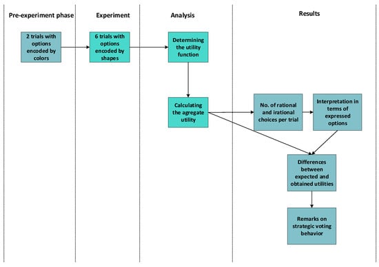
Figure 3.
The general scheme of the case study.
The basic voting idea consisted in the fact that the participants could vote during each iteration for one out of five options. Each option received a position on a spectrum of preferences. There were two extreme options, one centrist and two moderate options. This distribution was chosen in order to simulate a spectrum of political ideas as the one typically used nowadays, with a right and a left wing.
The pre-experiment phase consisted of two trials in which the political options were encoded by colors as shown in Table 9. The need for this phase is acknowledged by the scientific literature [,] and it represents one of the most critical phases in the success of an experiment. In this phase, any gaps in the design of the experiment can be observed and solved in order to ensure the success of the experimental phase. In our case, during this phase, it was observed that the participants associated the colors with real political parties, which led to a serious distortion of the results, making them unusable. In order to prevent such distortions in the other trials the options were encoded using geometrical shapes which carry no obvious political meaning. As no other issues were detected in this phase, other than the association of color with real parties, this was the only change we have made on the voting tickets we used in the experiment phase. The tickets can be seen in Appendix A.
Table 9.
Comparison between the shapes and colors used on the cards during the experiment.
In the experiment phase, in order to guarantee that preferences for each option were uniformly distributed, each participant received a card with written preferences for the geometrical shapes and the scores associated with the victory of each shape. Each participant had on their card a favorite choice which would bring them the most amount of points if that particular party received the highest number of votes. The number of points received would decrease linearly based on the distance between the winning option and the voter’s favorite option. Appendix B presents some voting options expressed during the experiment by various participants.
Table 10 describes the number of points received by the participants based on the card they received, and the winning option for the first set of cards which was used in the first two trials.
Table 10.
Matrix description of utilities for the first set of trials.
The first set of utilities featured asymmetric payoff values with respect to the positive/negative results. As can be observed in Table 10, only one of the five options had a positive score equal to one, while the majority of the values range in the negative area. As a result, the asymmetric payoff function with only one positive value used in the pre-experiment phase lead to the misconception that only that choice was rational.
As a result, in the second set of trials the utilities were selected in both a symmetrical and asymmetrical manner with respect to the positive/negative values spreading, while the second option, and sometimes the third option (please see cards 2, 3 and 4 in Table 11), had a positive score. Regarding the payoffs on each card, it can be observed that some of them are symmetric, while others are asymmetric, in order to better express the intensity of preferences, which can vary in practice from person to person []. Table 11 shows the score distributions after the second encoding was used.
Table 11.
Matrix description of utilities for the second set of trials.
The linear decrease present in the utilities is maintained after the applied changes.
The utility functions attributed to each type of card are as follows:
- Card 1: 4*Square + 2*Circle − 2*Hexagon − 4*Empty Circle
- Card 2: 2*Square + 4*Circle + 2*Triangle − 2*Empty Circle
- Card 3: 2*Circle + 4*Triangle + 2*Hexagon
- Card 4: −2*Square + 2*Triangle + 4*Hexagon + 2*Empty Circle
- Card 5: −4*Square − 2*Circle + 2*Hexagon + 4*Empty Circle
Aggregate utility is different depending on the winning geometrical shape, as noted in Table 12.
Table 12.
Aggregate utility based on the winning shape.
The results above show that at an aggregate level, a win by Triangle maximizes utility. However, the option which maximizes the individual utility is different depending on the card that each participant in the study received.
The experiment was carried out in an iterative manner. At the beginning of the experiment each voter received a card containing a table detailing their preferences and another table in which they could mark their preferred option at each iteration. At this stage participants wrote their names on the cards. In order to ensure equal representation for each option, three cards of each type were distributed. Participants were told about the structure of the card and how they would receive points based on what shape won, not based on the shape they picked.
After explaining how the experiment worked, the first iteration began. Voters marked their choice on the first line of their cards and then the cards were collected and the votes counted. After the votes were counted, voters were told the results. The number of points won by each participant in the study was marked on each card. The cards were returned to the participants, each one receiving the card they used at the previous iteration. The process continued in this manner until the number of iterations had been reached.
The main feedback loop of the system is formed by the number of points received by each participant after each iteration. The voters have access to the number of points they received after the previous iteration. Depending on the result of the previous iteration, participants can choose to change their option. Access to the results of previous iterations offers a way for the system to adjust. Thus, the utility each participant received at the previous iteration controls the way the system adapts.
The system adjusts by a feedback mechanism based on the utility participants won in the previous iterations. By extending this observation to a real first-past-the-post election, it can be concluded that first-past-the-post systems are characterized by a feedback process after each election. For example, if the winner had a low percentage and the next two candidates were near each other, the voters may decide to support just one of them in order to overtake the winner.
The obtained results show the occurrence of Duverger’s law in a first-past-the-post-system. This observation is in line with other studies from the field, most of them made upon data extracted from the field after different elections took place []. As for the occurrence of strategic voting, the results obtained in the present study are supported by other papers from the field which have observed strategic voting [,], some of them even in other voting systems such as a dual-ballot (two-round) election system [].
Regarding the decision period, the current study is in line with the results obtained by Zhirnov [] in 2019, which stated that “both strategic and non-strategic voters need time to form and communicate their preferences over candidates”.
5. Results of the Case Study on the Strategic Behavior
To properly analyze the results, one needs to determine how many participants made economically irrational choices. An irrational choice is observed in the case in which a participant decides to choose a political party that brings him/her less utility than the expected value of the utility. The expected value of the utility was determined after each iteration. First, the vote share for each party was determined by dividing the number of votes received by each party by the total number of voters (15 in our case). The vote share was then replaced in the corresponding utility function of each participant. In the case in which a participant selected in an iteration a party which provided him/her with a smaller utility than the determined expected value of the utility, that participant was considered irrational.
The number of rational and irrational choices in each trial (from trial 3 to trial 6) is summarized in Appendix C, in Table A1, Table A2, Table A3 and Table A4. Considering all the results, the number of rational and irrational choices for each trial was determined, as presented in Table 13.
Table 13.
Total rational and irrational choices per trial.
Based on the results, it was observed that the largest number of irrational votes were recorded in the 6th trial, in both absolute and relative terms. As a result, it was decided to discard the results of the 6th trial in our analysis.
In the following, the results obtained from the 3rd, 4th and 5th trials are analyzed and discussed in depth.
• Analyzing the results of the 3rd trial
During the 3rd trial, the first three iterations were characterized by the fact that Triangle was the most voted option (Table 14). In the 4th iteration, Circle and Triangle won an equal number of votes, though in order to determine the winner, the participants were told that Triangle had one vote less than Circle. The remaining vote was reallocated to Square. Then, in the 5th iteration, Circle was again the most voted option, thus making more voters choose Hexagon in order to reestablish an equilibrium. The last two iterations were characterized by a competition between two main options, Circle and Hexagon. This result can be noticed by the low number of votes for other options. In conclusion, at the end of the 3rd trial there were two opposed main options remaining as parties with a chance to win.
Table 14.
The results of the 3rd trial.
• Analyzing the results of the 4th trial
The 4th trial had a similar pattern in which a concentration around a central option is replaced by a consolidation of two main options. The last three iterations are characterized by a competition between Circle and Hexagon. In this trial, the concentration of the results in the last iterations is more pronounced than in the preceding trial (Table 15). In the 6th iteration all votes were in favor of only two options. The fact that the number of votes for Triangle reached zero is quite hard to explain, considering the utilities written on the cards. For the participants who received a card in which Triangle was the option which brought the most points, a victory for Circle brought the same number of points as a victory for Hexagon, so as long as none of the “extreme” options—namely Square or Empty Circle—had a chance of winning, the participants having a card in which Triangle was the preferred option should have had no reason to vote for another shape. Thus, their votes for Circle or Hexagon could be explained by the desire to vote for a winning option.
Table 15.
The results of the 4th trial.
• Analyzing the results of the 5th trial
In the 5th trial the winning option in the first iteration was Empty Circle, which led to different voter behavior (Table 16). The two main options are not stable and may change from one iteration to another. Moreover, the number of votes recorded for the most voted two options remains generally lower than in the case of the other trials.
Table 16.
The results of the 5th trial.
• Analyzing the voters’ behavior
One important note observed throughout the experiment is that as the participants become more experienced with the voting systems (as the number of voting iterations increased), they engage more in tactical voting in order to maximize their utilities.
For a better understanding of how the voters behaved, in the following, the results for the 4th trial are analyzed in depth.
The participants who received Empty Circle cards (cards on which the Empty Circle was the favorite choice) began by voting Triangle or Empty Circle and then gradually changed their options to Hexagon or Empty Circle (Table 17). As they observed that their favorite option had less and less chance of winning, they switched their voting option to their next preferred one on their list. This behavior implies that they tried not only to maximize their utilities, but also to minimize loss.
Table 17.
The options expressed by voters for whom Empty Circle brought the largest utility.
The voters who most preferred Hexagon swung between Triangle, Empty Circle and Hexagon in the first four iterations. In the last iteration the participants stabilized their choice on Hexagon (Table 18). This behavior is explained by Hexagon’s victory in the last iterations, which made the subjects whose favorite candidate was Hexagon vote continuously for Hexagon in order to ensure that it continued to win.
Table 18.
The options expressed by voters for whom Hexagon brought the largest utility.
The behavior observed above implies that once stabilized, a two-party system is hard to dismantle under a first-past-the-post system due to the fact that voters of entrenched parties lack incentives to vote for other parties in normal circumstances.
Generally, voters whose favorite candidate was Triangle chose it as long as it was in a winning position (Table 19). When the party was no longer winning, these participants switched to the next two favorite options (Hexagon and Circle). From a score standpoint, as long as the two most voted options were Circle and Hexagon, voters for whom Triangle brought the most points should have voted Triangle because the Circle and the Hexagon were indifferent for them and a win for Triangle would bring them more points. Nevertheless, in the last iterations these voters preferred to vote Circle or Hexagon. This behavior can be explained by the participants’ desire to select the winning candidate between two parties which are indifferent for them in terms of winning.
Table 19.
The options expressed by voters for whom Triangle brought the largest utility.
The participants who received cards 10 and 11 voted only Circle after the third iteration (Table 20). After Circle started being a possibly winning option, they stabilized their choice around this party. The voter who received card number 12 voted alternatively Circle and Hexagon in the last iteration. This behavior may imply that they did not understand properly the way points were given.
Table 20.
The options expressed by voters for whom Circle brought the largest utility.
The voters for whom Square brought most points switched between Square, Circle and Triangle in the first three iterations, after which they stabilized in their choice of Circle (Table 21). Considering this behavior, it was assumed that the participants with Square as a winning party probably preferred limiting loss by preventing a candidate positioned farther away from their political view from winning.
Table 21.
The options expressed by voters for whom Square brought the largest utility.
Table 22 summarizes the utilities each voter would receive if the party they picked at each round won, also called “expected utilities”. Considering the values from Table 22, it can be observed that all the values are nonnegative, except for one. The expected total is determined as the sum of the expected utilities in all the iterations for each party on each trial. The larger this value, the more consistent a voter was in picking their preferred option. It can be observed that the totals in the last column are smaller when participants chose options that would bring them a smaller utility if their party won the elections. It can also be noted that voters with cards where Square or Empty Circle were the preferred options had lower totals in the last column than the others. This result can be attributed to the fact that these participants needed to resort more to tactical voting.
Table 22.
Expected utilities.
Table 23 presents the obtained utilities. It can be observed that in the 4th trial the voters having cards that indicated Triangle as the most favorable option won the most points. The next-in-line voters were those with preferences for Circle or Hexagon. The least points were won by the participants with a high preference for Square or Empty Circle.
Table 23.
Obtained utilities.
As the total number of points gathered by a participant did not depend directly on his/her choices but on the party winning each set, a series of differences between the expected and the obtained utilities can be encountered. These differences are presented in Table 24.
Table 24.
Differences between expected and obtained utilities.
Considering the results in Table 24, it can be observed that some of the largest deviations were in the case in which the participants had cards where Square or Empty Circle were the options bringing most points. The smallest deviations were registered in the case in which the participants had Triangle as their preferred option. The people preferring Triangle had an in-built advantage due to the fact that whichever shape won they could not lose points. Table 25 notes how the participants changed their choices based on the utility of the previous iteration.
Table 25.
The number of cases in which the participants changed their option and the number of cases in which they did not change their options based on the utility received at the previous iteration.
Base on the data in Table 25, it can be seen that the people who won four points at a previous iteration were less willing to change their choice. Moreover, in relative terms, subjects receiving zero points were the most prone to change their voting decision.
6. Concluding Remarks and Discussions
During the experiment tactical voting could be observed. The results generally led to the formation of two opposed camps. The voters were prone to choosing an option with a smaller potential utility in order to stop less advantageous options from winning, thus balancing the potential utility with the chance of winning that a shape had. The potential of a shape (representing a party) to win would have little or no impact in a proportional system, thus making such calculations specific to the first-past-the-post system itself.
During the trials, results generally stabilized around two options. This happened in the last iterations of the trials. The voters needed time in order to adapt to the system and develop strategies to maximize their utilities. The feedback they received after each iteration, by means of the points received, played a part in how they developed their strategies, as can be seen in the table above. Those receiving a lower number of points were more prone to changing their choices.
The polarization around two options in the later iterations of the trials shows that after the participants get used to the first-past-the-post system, they start voting tactically. In the long term, this reinforces the advantages of the two main parties, making the smaller ones appear unelectable. It has also been observed that, during the experiment, some voters tended to change their options in favor of the party bringing the second largest number of points.
Considering the pitfalls of the experiment, one can name a pitfall caused by one of the assumptions: assuming each shape (party) to have an equal number of subjects preferring it is unrealistic, but considering the purely theoretical nature of the question posed, this limitation should not change the concluding remarks too much.
Another limitation of the experiment could be linked to the linear decrease of the utility on each card. The linear function was chosen in order to have a simple way of explaining and computing the results as the iterations were conducted. In order to have an empirical utility function, it would be necessary to conduct interviews with people to establish utility functions based on their responses.
In conclusion, during the experiment, tactical voting was observed. It was also observed that voters tend to take into account a candidate’s chance of winning when evaluating who to vote for under a first-past-the-post system. A low electability of their favorite candidate made voters vote for a candidate they would not consider as their first choice at the beginning of the experiments, but they did this in order to stop a candidate with a diametrically opposed ideological position from winning.
This leads to the idea that first-past-the-post systems lead to two-party political systems at the national level, not being favorable for small or new parties which might lose some of their electors due to the tactical voting the electors might exhibit. This can be regarded as a good outcome or, on the contrary, as a not-so-good outcome depending on the involved parties’ point of view. No matter the opinion of the involved parties, the rise of such behavior should be considered when trying to build and use a democratic voting system.
In addition, besides the phenomenon of learning from the rules of the voting system, another key mechanism may arise during the voting process with real candidates: the voting iterations might reveal the distribution of the preferences across the other respondents, which is beneficial to and highly exploited by electoral campaigns. Polling, for instance, tells voters which two candidates/parties are in the lead and which are likely to be beaten. As a result, a further extension of this study would be to consider a real voting situation, with candidates well known by the electors, and to try to separate the occurrence of the two mechanisms and their influence on the overall voters’ decision. For this purpose, we aim to extend the current study and implement an agent-based model in order to simulate the voters’ behavior in large populations.
Another possible extension would be to consider for a further experiment a case in which each participant receives a different utility matrix in a manner similar to the approach proposed by Blais et al. []. Additionally, larger groups of participants in the experiment can be considered.
Author Contributions
Conceptualization, A.C.; data curation, A.C. and C.D.; formal analysis, A.C. and C.D.; investigation, A.C. and C.D.; methodology, A.C.; software, A.C.; supervision, C.D.; Validation, C.D.; writing—original draft, A.C.; writing—review and editing, C.D. All authors have read and agreed to the published version of the manuscript.
Funding
This research received no funding.
Conflicts of Interest
The authors declare no conflict of interest.
Appendix A
The Voting Cards used in the Experiment phase.

Figure A1.
The content of Card 1 used in the Experiment phase.

Figure A2.
The content of Card 2 used in the Experiment phase.

Figure A3.
The content of Card 3 used in the Experiment phase.

Figure A4.
The content of Card 4 used in the Experiment phase.

Figure A5.
The content of Card 5 used in the Experiment phase.
Appendix B
Example of filled-in cards during the Experiment phase.

Figure A6.
Example of filled-in Card 3 (1).

Figure A7.
Example of filled-in Card 3 (2).

Figure A8.
Example of filled-in Card 3 (3).

Figure A9.
Example of filled-in Card 2.
Appendix C
Data extracted in different trials during the Experiment phase.
Table A1.
The number of rational and irrational choices for the third trial.
Table A1.
The number of rational and irrational choices for the third trial.
| Square | Circle | Triangle | Hexagon | Empty Circle | ||||||
|---|---|---|---|---|---|---|---|---|---|---|
| Choices over Expected Value | Choices under Expected Value * | Choices over Expected Value | Choices under Expected Value * | Choices over Expected Value | Choices under Expected Value * | Choices over Expected Value | Choices under Expected Value * | Choices over Expected Value | Choices under Expected Value * | |
| Iteration 2 | 2 | 1 | 3 | 0 | 2 | 1 | 3 | 0 | 2 | 1 |
| Iteration 3 | 3 | 0 | 3 | 0 | 2 | 1 | 3 | 0 | 1 | 2 |
| Iteration 4 | 3 | 0 | 3 | 0 | 2 | 1 | 3 | 0 | 2 | 1 |
| Iteration 5 | 3 | 0 | 2 | 1 | 2 | 1 | 3 | 0 | 3 | 0 |
| Iteration 6 | 3 | 0 | 3 | 0 | 1 | 2 | 3 | 0 | 2 | 1 |
| Iteration 7 | 3 | 0 | 3 | 0 | 1 | 2 | 3 | 0 | 2 | 1 |
* Equal to irrational behavior.
Table A2.
The number of rational and irrational choices for the fourth trial.
Table A2.
The number of rational and irrational choices for the fourth trial.
| Square | Circle | Triangle | Hexagon | Empty Circle | ||||||
|---|---|---|---|---|---|---|---|---|---|---|
| Choices over Expected Value | Choices under Expected Value * | Choices over Expected Value | Choices under Expected Value * | Choices over Expected Value | Choices under Expected Value * | Choices over Expected Value | Choices under Expected Value * | Choices over Expected Value | Choices under Expected Value * | |
| Iteration 2 | 3 | 0 | 2 | 1 | 3 | 0 | 3 | 0 | 3 | 0 |
| Iteration 3 | 3 | 0 | 3 | 0 | 2 | 1 | 3 | 0 | 3 | 0 |
| Iteration 4 | 3 | 0 | 3 | 0 | 2 | 1 | 3 | 0 | 2 | 1 |
| Iteration 5 | 3 | 0 | 2 | 1 | 3 | 0 | 3 | 0 | 3 | 0 |
| Iteration 6 | 3 | 0 | 3 | 0 | 0 | 3 | 3 | 0 | 3 | 0 |
| Iteration 7 | 3 | 0 | 2 | 1 | 0 | 3 | 3 | 0 | 3 | 0 |
* Equal to irrational behavior.
Table A3.
The number of rational and irrational choices for the fifth trial.
Table A3.
The number of rational and irrational choices for the fifth trial.
| Square | Circle | Triangle | Hexagon | Empty Circle | ||||||
|---|---|---|---|---|---|---|---|---|---|---|
| Choices over Expected Value | Choices under Expected Value * | Choices over Expected Value | Choices under Expected Value * | Choices over Expected Value | Choices under Expected Value * | Choices over Expected Value | Choices under Expected Value * | Choices over Expected Value | Choices under Expected Value * | |
| Iteration 2 | 3 | 0 | 3 | 0 | 3 | 0 | 3 | 0 | 3 | 0 |
| Iteration 3 | 2 | 1 | 3 | 0 | 3 | 0 | 3 | 0 | 3 | 0 |
| Iteration 4 | 3 | 0 | 3 | 0 | 3 | 0 | 3 | 0 | 3 | 0 |
| Iteration 5 | 3 | 0 | 3 | 0 | 3 | 0 | 3 | 0 | 3 | 0 |
| Iteration 6 | 3 | 0 | 1 | 2 | 0 | 3 | 3 | 0 | 2 | 1 |
| Iteration 7 | 2 | 1 | 3 | 0 | 3 | 0 | 3 | 0 | 3 | 0 |
* Equal to irrational behavior.
Table A4.
The number of rational and irrational choices for the sixth trial.
Table A4.
The number of rational and irrational choices for the sixth trial.
| Square | Circle | Triangle | Hexagon | Empty Circle | ||||||
|---|---|---|---|---|---|---|---|---|---|---|
| Choices over Expected Value | Choices under Expected Value * | Choices over Expected Value | Choices under Expected Value * | Choices over Expected Value | Choices under Expected Value * | Choices over Expected Value | Choices under Expected Value * | Choices over Expected Value | Choices under Expected Value * | |
| Iteration 2 | 1 | 2 | 0 | 3 | 3 | 0 | 3 | 0 | 2 | 1 |
| Iteration 3 | 3 | 0 | 3 | 0 | 2 | 1 | 1 | 2 | 3 | 0 |
| Iteration 4 | 2 | 1 | 3 | 0 | 1 | 2 | 2 | 1 | 1 | 2 |
| Iteration 5 | 2 | 1 | 1 | 2 | 1 | 2 | 3 | 0 | 2 | 1 |
| Iteration 6 | 2 | 1 | 3 | 0 | 2 | 1 | 3 | 0 | 3 | 0 |
| Iteration 7 | 2 | 1 | 3 | 0 | 3 | 0 | 3 | 0 | 3 | 0 |
| Iteration 8 | 3 | 0 | 3 | 0 | 3 | 0 | 3 | 0 | 3 | 0 |
* Equal to irrational behavior.
References
- Martínez-Panero, M.; Arredondo, V.; Peña, T.; Ramírez, V. A New Quota Approach to Electoral Disproportionality. Economies 2019, 7, 17. [Google Scholar] [CrossRef]
- Hizen, Y. Does a Least-Preferred Candidate Win a Seat? A Comparison of Three Electoral Systems. Economies 2015, 3, 2–36. [Google Scholar] [CrossRef]
- Bizzotto, J.; Solow, B. Electoral Competition with Strategic Disclosure. Games 2019, 10, 29. [Google Scholar] [CrossRef]
- Pérez-Fernández, R.; García-Lapresta, J.L.; De Baets, B. Chronicle of a Failure Foretold: 2017 Rector Election at Ghent University. Economies 2019, 7, 2. [Google Scholar] [CrossRef]
- Potthoff, R.F. Three Bizarre Presidential-Election Scenarios: The Perils of Simplism. Soc. Sci. 2019, 8, 134. [Google Scholar] [CrossRef]
- Tso, R.; Liu, Z.-Y.; Hsiao, J.-H. Distributed E-Voting and E-Bidding Systems Based on Smart Contract. Electronics 2019, 8, 422. [Google Scholar] [CrossRef]
- Thompson, J. A Review of the Popular and Scholarly Accounts of Donald Trump’s White Working-Class Support in the 2016 US Presidential Election. Societies 2019, 9, 36. [Google Scholar] [CrossRef]
- Zou, X.; Li, H.; Li, F.; Peng, W.; Sui, Y. Transparent, Auditable, and Stepwise Verifiable Online E-Voting Enabling an Open and Fair Election. Cryptography 2017, 1, 13. [Google Scholar] [CrossRef]
- Boyen, X.; Haines, T. Forward-Secure Linkable Ring Signatures from Bilinear Maps. Cryptography 2018, 2, 35. [Google Scholar] [CrossRef]
- Kamijo, Y.; Hizen, Y.; Saijo, T.; Tamura, T. Voting on Behalf of a Future Generation: A Laboratory Experiment. Sustainability 2019, 11, 4271. [Google Scholar] [CrossRef]
- Ehsan, M. What Matters? Non-Electoral Youth Political Participation in Austerity Britain. Societies 2018, 8, 101. [Google Scholar] [CrossRef]
- Zeedan, R. The 2016 US Presidential Elections: What Went Wrong in Pre-Election Polls? Demographics Help to Explain. Multidiscip. Sci. J. 2019, 2, 84–101. [Google Scholar] [CrossRef]
- Lijphart, A. Democracies: Forms, performance, and constitutional engineering. Eur. J. Political Res. 1994, 25, 1–17. [Google Scholar] [CrossRef]
- Cox, G.W. Making Votes Count: Strategic Coordination in the World’s Electoral Systems, 1st ed.; Cambridge University Press: San Diego, CA, USA, 1997; ISBN 978-0-521-58516-3. [Google Scholar]
- Norris, S. Analyzing Multimodal Interaction: A Methodological Framework, 1st ed.; Routledge: New York, NY, USA, 2004; ISBN 978-0-203-37949-3. [Google Scholar]
- Endersby, J.W.; Shaw, K.B. Strategic Voting in Plurality Elections: A Simulation of Duverger’s Law. PS Political Sci. Politics 2009, 42, 393–399. [Google Scholar] [CrossRef]
- Rich, T.S. Duverger’s Law in mixed legislative systems: The impact of national electoral rules on district competition: Duverger’s Law in mixed legislative systems. Eur. J. Political Res. 2015, 54, 182–196. [Google Scholar] [CrossRef]
- Clark, W.R.; Golder, M. Rehabilitating Duverger’s Theory: Testing the Mechanical and Strategic Modifying Effects of Electoral Laws. Comp. Political Stud. 2006, 39, 679–708. [Google Scholar] [CrossRef]
- Chhibber, P.; Kollman, K. The Formation of National Party Systems: Federalism and Party Competition in Canada, Great Britain, India, and the United States; Princeton University Press: Princeton, NJ, USA, 2004; ISBN 978-0-691-11932-8. [Google Scholar]
- Fujiwara, T. A Regression Discontinuity Test of Strategic Voting and Duverger’s Law. Qrs. J. Political Sci. 2011, 6, 197–233. [Google Scholar] [CrossRef]
- Blais, A. To Keep or to Change First Past the Post? Oxford University Press: Oxford, UK, 2008; ISBN 978-0-19-953939-0. [Google Scholar]
- Downs, A. An Economic Theory of Political Action in a Democracy. J. Political Econ. 1957, 65, 135–150. [Google Scholar] [CrossRef]
- Norton, P. The case for First-Past-The-Post. Representation 1997, 34, 84–88. [Google Scholar] [CrossRef]
- Blais, A.; Pilet, J.-B.; Van der Straeten, K.; Laslier, J.-F.; Héroux-Legault, M. To vote or to abstain? An experimental test of rational calculus in first past the post and PR elections. Elect. Stud. 2014, 36, 39–50. [Google Scholar] [CrossRef]
- Bogdanor, V. First-Past-The-Post: An electoral system which is difficult to defend. Representation 1997, 34, 80–83. [Google Scholar] [CrossRef]
- Moser, R.G.; Scheiner, E.; Milazzo, C. Social Diversity Affects the Number of Parties Even Under First Past the Post Rules; Social Science Research Network: Rochester, NY, USA, 2011. [Google Scholar]
- Milazzo, C.; Moser, R.G.; Scheiner, E. Social Diversity Affects the Number of Parties Even Under First-Past-the-Post Rules. Comp. Political Stud. 2018, 51, 938–974. [Google Scholar] [CrossRef]
- Laycock, S.; Renwick, A.; Stevens, D.; Vowles, J. The UK’s electoral reform referendum of May 2011. Elect. Stud. 2013, 32, 211–214. [Google Scholar] [CrossRef]
- Bochsler, D. The strategic effect of the plurality vote at the district level. Elect. Stud. 2017, 47, 94–112. [Google Scholar] [CrossRef]
- Vowles, J. The Manipulation of Norms and Emotions? Partisan Cues and Campaign Claims in the UK Electoral System Referendum; Social Science Research Network: Rochester, NY, USA, 2011. [Google Scholar]
- Pilon, D. Review Essay-Democratic Leviathan: Defending First-Past-the-Post in Canada. Can. Political Sci. Rev. 2018, 12, 24–49. [Google Scholar]
- Maškarinec, P. The 2016 Electoral Reform in Mongolia: From Mixed System and Multiparty Competition to FPTP and One-Party Dominance. J. Asian Afr. Stud. 2018, 53, 511–531. [Google Scholar] [CrossRef]
- Levine, D.K.; Palfrey, T.R. The paradox of voter participation? A laboratory study. Am. Political Sci. Rev. 2007, 101, 143–158. [Google Scholar] [CrossRef]
- Palfrey, T.R.; Rosenthal, H. Voter Participation and Strategic Uncertainty. Am. Political Sci. Rev. 1985, 79, 62–78. [Google Scholar] [CrossRef]
- Riker, W. Duverger’s Law Revisited. In Electoral Laws and Their Political Consequences; Agathon Press: New York, NY, USA, 2003; p. 19. [Google Scholar]
- Schram, A.; Sonnemans, J. Voter turnout as a participation game: An experimental investigation. Int. J. Game Theory 1996, 25, 385–406. [Google Scholar] [CrossRef]
- Schram, A.; Sonnemans, J. Why people vote: Experimental evidence. J. Econ. Psychol. 1996, 17, 417–442. [Google Scholar] [CrossRef]
- Duffy, J.; Tavits, M. Beliefs and Voting Decisions: A Test of the Pivotal Voter Model. Am. J. Political Sci. 2008, 52, 603–618. [Google Scholar] [CrossRef]
- Herrera, H.; Morelli, M.; Palfrey, T. Turnout and Power Sharing. Econ. J. 2014, 124, 131–162. [Google Scholar] [CrossRef]
- Kartal, M. Laboratory elections with endogenous turnout: Proportional representation versus majoritarian rule. Exp. Econ. 2015, 18, 366–384. [Google Scholar] [CrossRef]
- Cooter, R. The Strategic Constitution; Princeton University Press: Princeton, NJ, USA, 2002; ISBN 978-0-691-09620-9. [Google Scholar]
- Reeve, A.; Ware, A. Electoral Systems: A Comparative and Theoretical Introduction (Theory and Practice in British Politics); Routledge: London, UK, 1992; ISBN 978-0-415-01204-1. [Google Scholar]
- Curtice, J. Neither Representative nor Accountable: First-Past-the-Post in Britain. In Duverger’s Law of Plurality Voting, 13th ed.; Springer: New York, NY, USA, 2009; pp. 27–45. ISBN 978-0-387-09719-0. [Google Scholar]
- BBC 2017 Elections Results. Available online: https://www.bbc.com/news/election/2017/results (accessed on 3 October 2019).
- Bowler, S.; Donovan, T.; van Heerde, J. The United States of America: Perpetual Campaigning in the Absence of Competition. In The Politics of Electoral Systems; Gallagher, M., Mitchell, P., Eds.; Oxford University Press: New York, NY, USA, 2005; pp. 185–206. ISBN 978-0-19-925756-0. [Google Scholar]
- Mackie, T.T.; Rose, R. The International Almanac of Electoral History, 3rd ed.; Macmillan: Basingstoke, UK, 1991; ISBN 978-0-333-45279-0. [Google Scholar]
- US Goverment The Constitution of the United States: A Transcription. Available online: https://www.archives.gov/founding-docs/constitution-transcript (accessed on 3 October 2019).
- Barten, A.P. Consumer Economics. In International Encyclopedia of the Social & Behavioral Sciences; Elsevier: New York, NY, USA, 2001; pp. 2669–2674. ISBN 978-0-08-043076-8. [Google Scholar]
- Rébillé, Y. Representations of preferences with pseudolinear utility functions. J. Math. Psychol. 2019, 89, 1–12. [Google Scholar] [CrossRef]
- Weber, M. Risk: Theories of Decision and Choice. In International Encyclopedia of the Social & Behavioral Sciences; Elsevier: New York, NY, USA, 2001; pp. 13364–13368. ISBN 978-0-08-043076-8. [Google Scholar]
- Zhao, W.-X.; Ho, H.-P.; Chang, C.-T. The roles of aspirations, coefficients and utility functions in multiple objective decision making. Comp. Ind. Eng. 2019, 135, 227–235. [Google Scholar] [CrossRef]
- Blais, A.; Hortala-Vallve, R. Are People More or Less Inclined to Vote When Aggregate Turnout Is High? In Voting Experiments; Blais, A., Laslier, J.-F., Van der Straeten, K., Eds.; Springer International Publishing: Cham, Switzerland, 2016; pp. 117–125. ISBN 978-3-319-40571-1. [Google Scholar]
- Farooq, M.A.; Nóvoa, H.; Araújo, A.; Tavares, S.M.O. An innovative approach for planning and execution of pre-experimental runs for Design of Experiments. Eur. Res. Manag. Bus. Econ. 2016, 22, 155–161. [Google Scholar] [CrossRef]
- Nijman, T.; Verbeek, M. The optimal choice of controls and pre-experimental observations. J. Econ. 1992, 51, 183–189. [Google Scholar] [CrossRef][Green Version]
- Alvarez, R.M.; Boehmke, F.J.; Nagler, J. Strategic voting in British elections. Elect. Stud. 2006, 25, 1–19. [Google Scholar] [CrossRef]
- Herrmann, M.; Pappi, F.U. Strategic voting in German constituencies. Elect. Stud. 2008, 27, 228–244. [Google Scholar] [CrossRef]
- Kiss, Á. Identifying strategic voting in two-round elections. Elect. Stud. 2015, 40, 127–135. [Google Scholar] [CrossRef]
- Zhirnov, A. Decision period and Duverger’s psychological effect in FPTP elections: Evidence from India. Elect. Stud. 2019, 58, 21–30. [Google Scholar] [CrossRef]
© 2020 by the authors. Licensee MDPI, Basel, Switzerland. This article is an open access article distributed under the terms and conditions of the Creative Commons Attribution (CC BY) license (http://creativecommons.org/licenses/by/4.0/).