A New Quasi Cubic Rational System with Two Parameters


Abstract
:1. Introduction
2. Preliminaries
3. Main Results
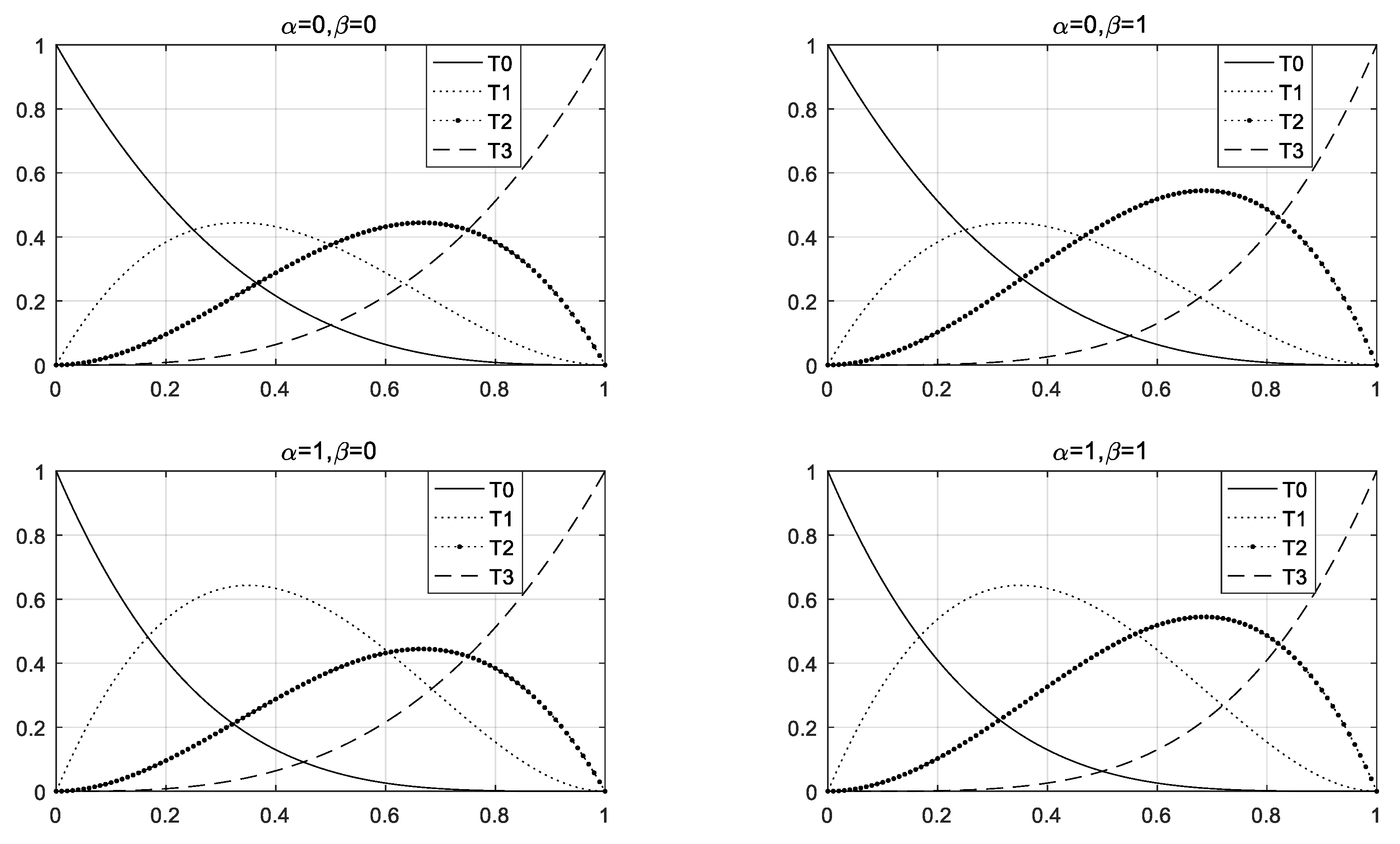
3.1. Construction of the QCR-B System
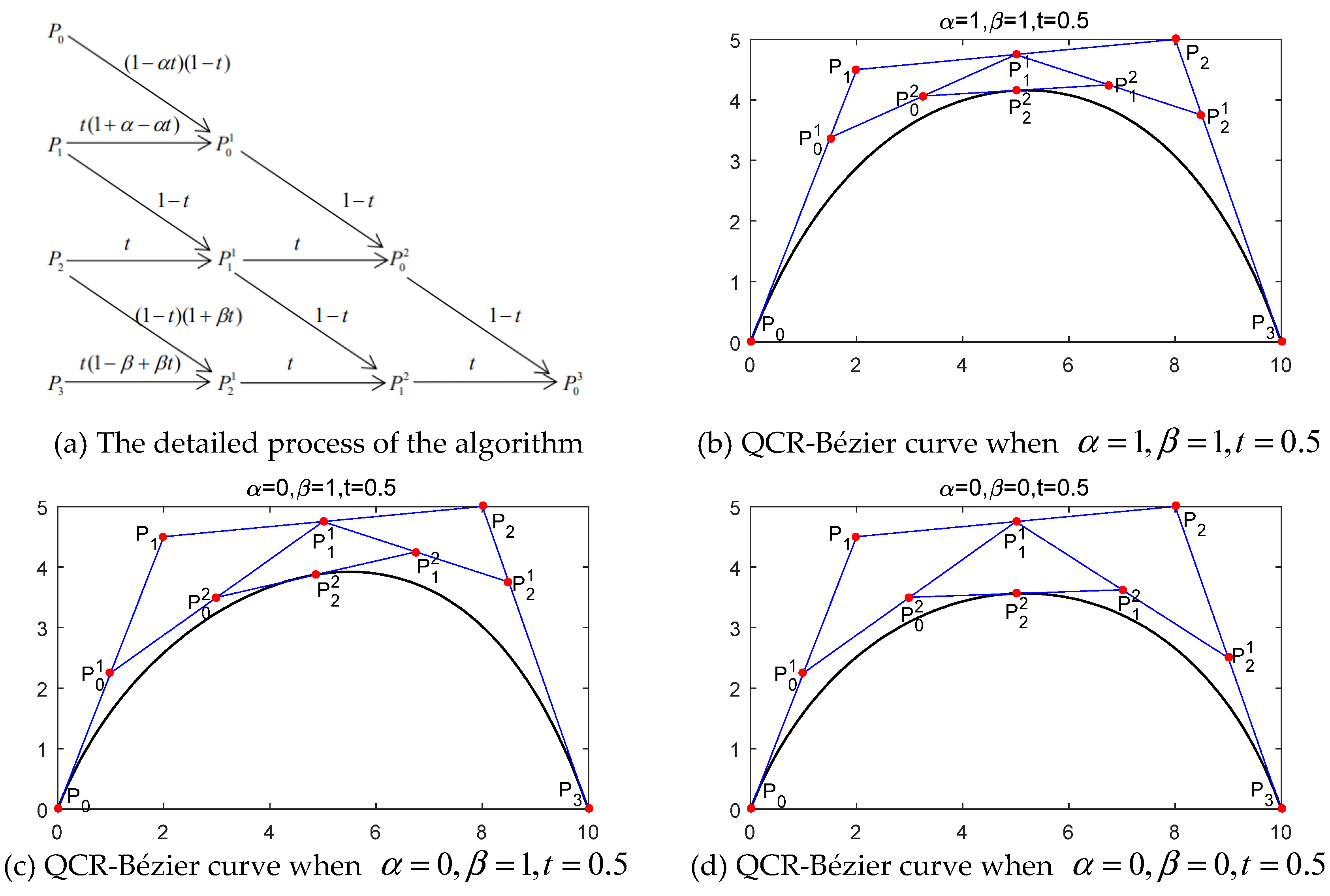
3.2. QCR-Bézier Curve
3.3. Non-Uniform QCR-B Spline Curves and Their Applications
3.3.1. Structure of the Non-Uniform QCR-B Spline System
3.3.2. Properties of the Non-Uniform QCR-B Spline System
- (1)
- Unity: For any , .
- (2)
- Nonnegativity: For any , there is .
- (3)
- Symmetry: For any , we have:
- (4)
- Linear independence: For any , is linear independence on interval .
- (6)
- Continuity: Given a non-uniform knot vector, for any , has continuity at each knot.
3.4. Non-Uniform QCR-B Spline Curve
3.4.1. Definition and Properties
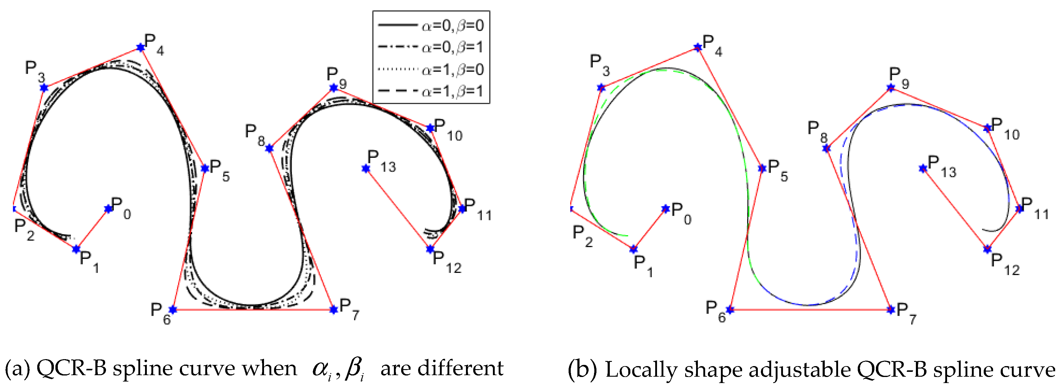
3.4.2. Local Adjustment
3.5. QCR-BB System over Triangular Domain
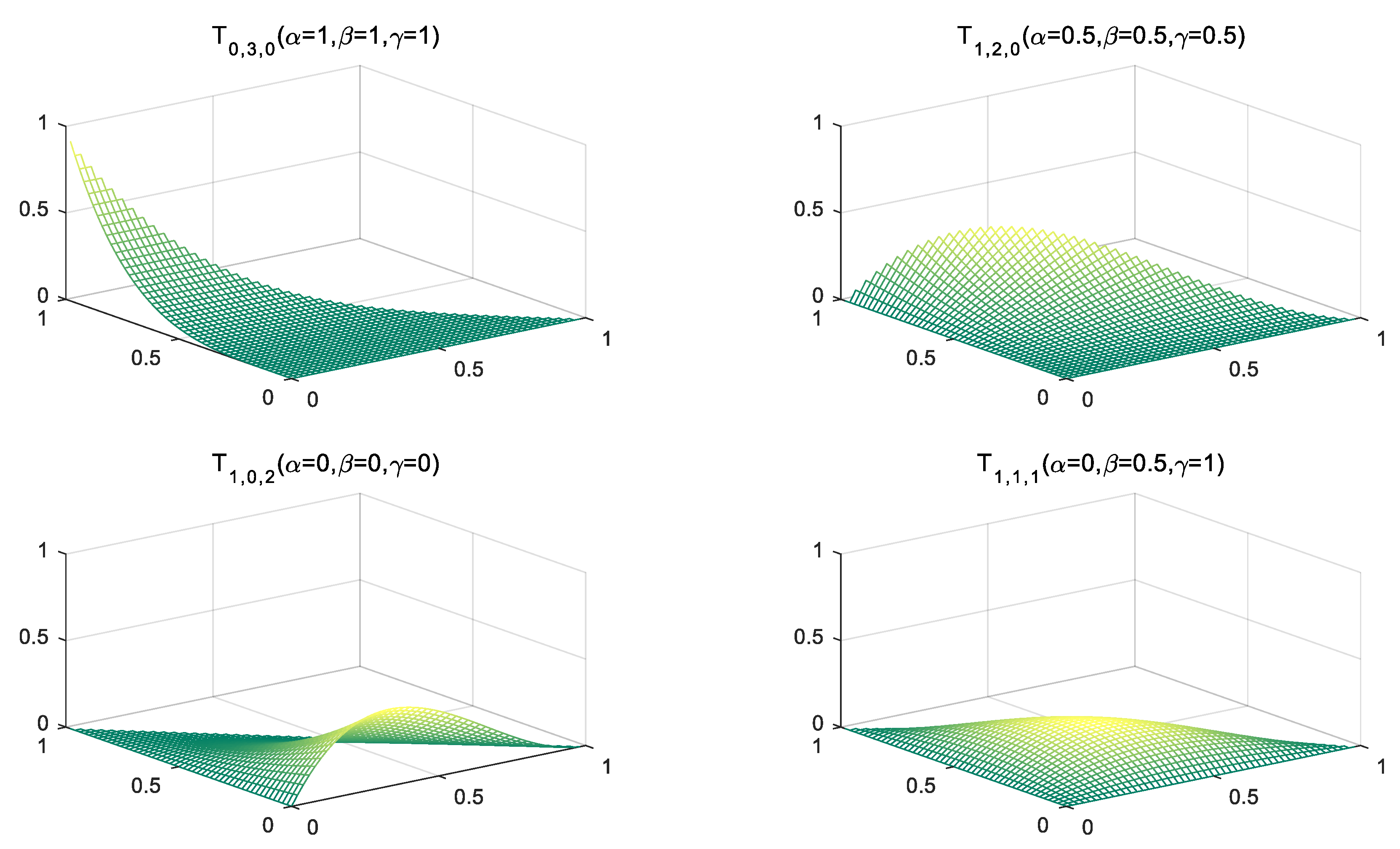
3.5.1. Construction of the QCR-BB System
3.5.2. Properties of the QCR-BB System
- (1)
- Nonnegativity: For any , there are
- (2)
- Unity:
- (3)
- Symmetry:
- (4)
- Boundary property:If , the ten system described in Equation (14) could degenerate to the QCR-Bernstein system given in Equation (1).
- (5)
- Linear independence: are linear independence.
3.5.3. The QCR-BB Patch
- (1)
- Convex hull and affine invariance: Given that the QCR-BB system has the unity and non-negativity, therefore, the QCR-BB patches have the property of convex hull and affine invariance.
- (2)
- Attribution of corner interpolation: By directly computing, that is:
- (3)
- Corner point tangent plane: Let , it can:
- (4)
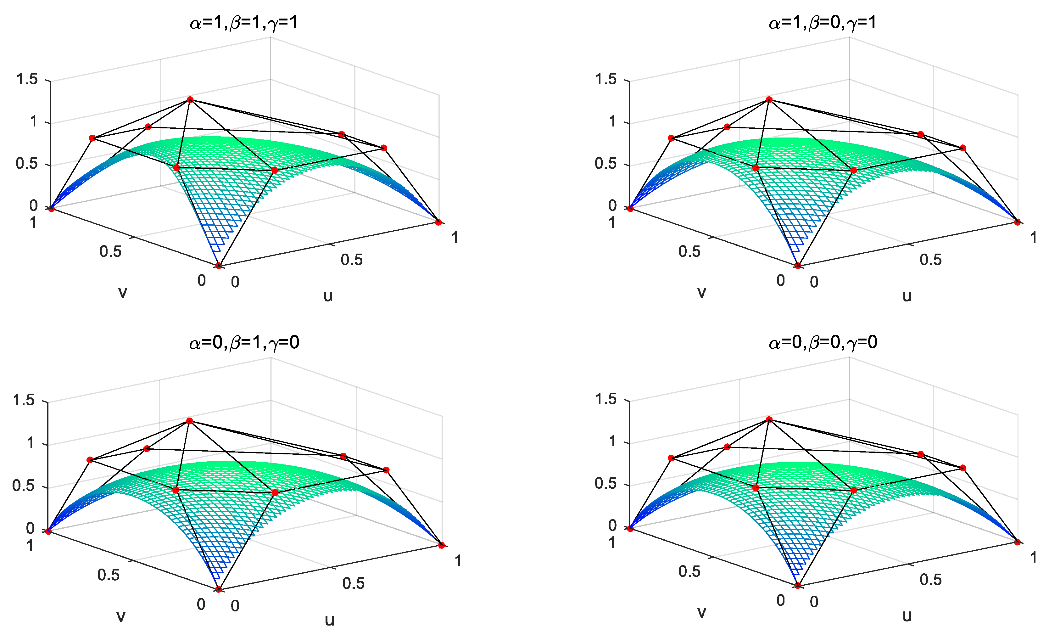
- Boundary property: When , degenerated into a QCR-Bézier curve with two parameters . When , degenerated into a QCR-Bézier curve with . When , degenerated into a QCR-Bézier curve with . With the values of , and increasing, the QCR-BB patch will be approached to the control mesh. Hence, the parameters , and have a tension effect.
- (5)
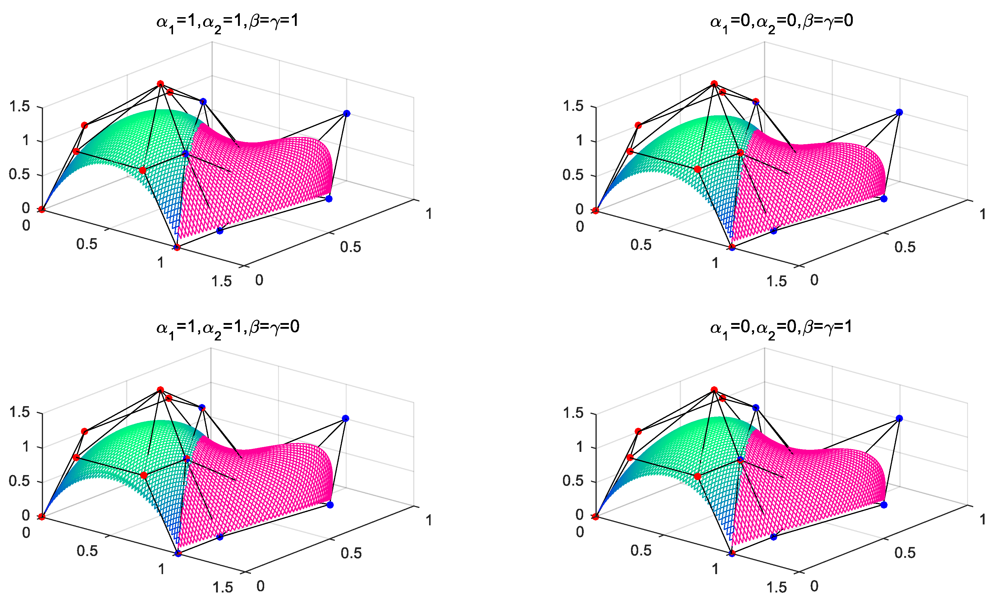
- Shape adjustability: The shape of the can be turned-up by modifying the value of the , and when the control mesh is stabled. With the values of , and increasing, the would approach to the control mesh. Hence, it is easy for us to get the parameters , and to have a tension effect. According to the boundary property of the , each boundary curve , and only have two related parameters. Thus, changing a parameter can only affect the shape of two boundary curves. Figure 7 shows the effects of different parameter values on the QCR-BB patch when the control mesh is fixed.
3.5.4. De Casteljau-Type Algorithm
3.5.5. Joining of QCR-BB Patches
4. Conclusions
Author Contributions
Funding
Conflicts of Interest
References
- Prautzsch, H.; Piper, B. A fast algorithm to raise the degree of spline curves. Comput. Aided Geom. Des. 1991, 8, 253–265. [Google Scholar] [CrossRef]
- Costantini, P. Curve and surface construction using variable degree polynomial splines. Comput. Aided Geom. Des. 2000, 17, 419–466. [Google Scholar] [CrossRef]
- Juhász, I.; Hoffmann, M. On the quartic curve of Han. J. Comput. Appl. Math. 2007, 223, 123–132. [Google Scholar] [CrossRef] [Green Version]
- Salomon, D.; Schneider, F.B. The Computer Graphics Manual; Springer: New York, NY, USA, 2011. [Google Scholar]
- Farin, G. Curves and Surfaces for CAGD: A Practical Guide, 5th ed.; Academic Press: San Diego, CA, USA, 2002; pp. 367–376. [Google Scholar]
- Oruc, H.; Phillips, G.H. q-Bernstein polynomials and Bézier curves. J. Comput. Math. 2003, 151, 1–12. [Google Scholar] [CrossRef] [Green Version]
- Chen, J.; Wang, G.J. Progressive iterative approximation for triangular Bézier sufaces. Comput. Aided Des. 2011, 43, 889–895. [Google Scholar] [CrossRef]
- Costantini, P.; Pelosi, F.; Sampoli, M.L. New spline spaces with generalized tension properties. BIT Numer. Math. 2008, 48, 665–688. [Google Scholar] [CrossRef]
- Xu, G.; Wang, G.Z. Extended cubic uniform B-spline and the cubic trigonometric Bézier curve with two shape parameters. Acta Autom. Sin. 2008, 34, 980–984. [Google Scholar] [CrossRef]
- Zhang, R.J. Uniform interpolation curves and surfaces based on a family of symmetric splines. Comput. Aided Geom. Des. 2013, 30, 844–860. [Google Scholar] [CrossRef]
- Delgado-Gonzalo, R.; Thévenaz, P.; Unser, M. Exponential splines and minimal-support bases for curve representation. Comput. Aided Geom. Des. 2011, 29, 109–128. [Google Scholar] [CrossRef] [Green Version]
- Chen, Q.Y.; Wang, G.Z. A class of Bézier-like curves. Comput. Aided Geom. Des. 2003, 20, 29–39. [Google Scholar] [CrossRef]
- Tea-wan, K.; Boris, K. A shape-preserving apporximation by weighted cubic splines. J. Comput. Appl. Math. 2012, 236, 4383–4397. [Google Scholar]
- Yan, L.L.; Han, X.L.; Huang, T. Cubic trigonometric polynomial curves and surfaces with a shape parameter. J. Comput. Aided Des. Comput. Graph. 2016, 28, 1047–1058. [Google Scholar]
- Wu, X.Q.; Han, X.L. Extension of cubic Bézier curve. J. Eng. Graph. 2005, 6, 98–102. [Google Scholar]
- Hu, G.; Ji, X.M.; Qin, X.Q. Quickly constuction of quartic λ-Bézier rotation surfaces with shape parameters. Trans. Chin. Soc. Agric. Mach. 2014, 45, 304–309. [Google Scholar]
- Hu, G.; Ji, X.M.; Guo, L. Quartic generalized Bézier surfaces with multiple shape parameters and its continuity conditions. Trans. Chin. Soc. Agric. Mach. 2014, 45, 315–321. [Google Scholar]
- Hu, G.; Song, W.J. New method for constructing quasi-Bézier rotation surfaces with multiple shape parameters. J. Xi’an Jiaotong Univ. 2014, 28, 74–79. [Google Scholar]
- Guo, L.; A, L.S.; Hu, G. Designing car body with blended cubic Q-Bézier surfaces. Mech. Sci. Technol. Aerosp. Eng. 2017, 36, 114–118. [Google Scholar]
- Juhász, I.; Róth, Á. A class of generalized B-spline curves. Comput. Aided Geom. Des. 2013, 30, 85–115. [Google Scholar] [CrossRef]
- Mazure, M.L. On dimension elevation in Quasi Extended Chebyshev spaces. Numer. Math. 2008, 109, 459–475. [Google Scholar] [CrossRef]
- Mazure, M.L. Quasi Extended Chebyshev spaces and weight functions. Numer. Math. 2011, 118, 79–108. [Google Scholar] [CrossRef]
- Bosner, T.; Rogina, M. Variable degree polynomial splines are Chebyshev splines. Adv. Comput. Math. 2013, 38, 383–400. [Google Scholar] [CrossRef]
- Carnicer, J.M.; Mainar, E.; Peña, J.M. Critical length for design purpose and extended Chebyshev spaces. Constr. Approx. 2003, 20, 55–71. [Google Scholar] [CrossRef]
- Mazure, M.L. Which spaces for design? Numer. Math. 2008, 110, 357–392. [Google Scholar] [CrossRef]
- Mazure, M.L. On a general new class of quasi Chebyshevian splines. Numer. Algorithms 2011, 58, 399–438. [Google Scholar] [CrossRef]
- Carnicer, J.M.; Peña, J.M. Total positive bases for shape preserving curve design and optimality of B-splines. Comput. Aided Geom. Des. 1994, 11, 633–654. [Google Scholar] [CrossRef]
- Mazure, M.L. Chebyshev spaces and Bernstein bases. Constr. Approx. 2005, 22, 347–363. [Google Scholar] [CrossRef]
- 29. Bernstein. S.N. Démonstration du théoème de Weierstrass fondée sur le calcul des probabilités. Comm. Soc. Math. Kharkow 1912, 13, 1–2.


© 2020 by the authors. Licensee MDPI, Basel, Switzerland. This article is an open access article distributed under the terms and conditions of the Creative Commons Attribution (CC BY) license (http://creativecommons.org/licenses/by/4.0/).
Share and Cite
Tuo, M.-X.; Zhang, G.-C.; Wang, K. A New Quasi Cubic Rational System with Two Parameters. Symmetry 2020, 12, 1070. https://doi.org/10.3390/sym12071070
Tuo M-X, Zhang G-C, Wang K. A New Quasi Cubic Rational System with Two Parameters. Symmetry. 2020; 12(7):1070. https://doi.org/10.3390/sym12071070
Chicago/Turabian StyleTuo, Ming-Xiu, Gui-Cang Zhang, and Kai Wang. 2020. "A New Quasi Cubic Rational System with Two Parameters" Symmetry 12, no. 7: 1070. https://doi.org/10.3390/sym12071070
APA StyleTuo, M.-X., Zhang, G.-C., & Wang, K. (2020). A New Quasi Cubic Rational System with Two Parameters. Symmetry, 12(7), 1070. https://doi.org/10.3390/sym12071070