1. Introduction
The outbreak of novel coronavirus called COVID-19 in China has attracted extensive attention of many scientists, in particular mathematicians working in mathematical modeling. The first papers were already published in February–April 2020 [
1,
2,
3,
4,
5,
6,
7,
8]. At the present time, the COVID-19 outbreak has already spread over the world as a pandemic. There were almost 4,000,000 coronavirus cases up to date 8 May [
9]. This work is a natural continuation of [
8], in which we used the measured data at the beginning of the pandemic.
At the present time, there are many mathematical models used to describe epidemic processes and they can be found in any book devoted to mathematical models in biology and medicine (see, e.g., Refs. [
10,
11,
12,
13] and papers cited therein). The paper [
14] is one of the first papers in this direction. The authors created a model based on three ordinary differential equations (ODEs), which presently is called the SIR model. There are several generalizations of the SIR model and the SEIR model (see the pioneering works [
15,
16]), which involves four ODEs, is the most common among them. These two models are mostly used for numerical simulations in mathematical modeling the COVID-19 outbreak (see, e.g., [
2,
4,
5]).
Our aim is to develop a simple mathematical model for the COVID-19 outbreak, which possesses two properties, namely one is integrable and one predicts results, which are relevant to the measured data. Of course, such kind of models cannot catch all features of this epidemic process, which is very complicated. However, the model provides good results without long and complicated numerical simulations. Moreover, it is possible to make some predictions with acceptable exactness.
The paper is organized as follows. In
Section 2, we propose a simple model, which was developed using the public data about the COVID-19 outbreak presented by WORLDOMETER [
9]. Then we generalize the model taking into account the known information that the mortality rate in several countries is rather high. Both model are based on nonlinear system of ODEs. We demonstrate that both models are exactly solvable.
In
Section 3, we demonstrate that the model describes very good the COVID-19 outbreak in China. This case was used because there are obvious indications that this epidemic threat was effectively removed in China. In
Section 4, the model is applied to the COVID-19 outbreak in Austria and Poland. It is shown that the degree of nonlinearity in the model varies from one country to another country. A prediction of the total number of the COVID-19 cases is also discussed and an example is presented using the measured data in Poland. We also demonstrate the applicability of the model to the COVID-19 outbreak in France, where the mortality rate is rather high.
Finally, some conclusions are presented and a nontrivial generalization of the model based on a nonlinear PDE system, which takes into account nonhomogeneous space distribution of the infected population, is suggested in
Section 5.
2. Mathematical Model
The first nontrivial biological model used for calculation and the time evolution of the total world population of people was created in 1838 by Verhulst [
17]. His model is usually called the logistic model and has the form (in dimensionless variables)
and is the classical example in any textbook on Mathematical Biology. Its exact solution is well known
and depending on the value
suggests three different scenarios for the population evolution. In particular, the useful curve, the so-called sigmoid, is obtained if
(see, e.g., Figure 1.1 in [
18]).
We have noted that the data [
9] for the total number of the COVID-19 cases in China and some other countries can be approximated by a sigmoid with the correctly specified parameters. Having this in mind, we introduce a smooth function
, which presents the total number of the COVID-19 cases identified up to day
t (for any integer number
t). We assume that the first case (cases)
was (were) identified at
Obviously, the function
is nondecreasing. Therefore, we obtain
where
a and
b are positive constants. One may define
a as
, where
is the infection rate and
S is an average number of healthy persons, who was contacted by a fixed infected person (the so-called mechanism of the virus transmission). Obviously, each infected person can be in contact only with a limited number of people (usually it is relatives and close friends). The term
has an opposite meaning to
a, because one reflects the efforts
B, in order to avoid contacts with infected persons and to make other restrictions introduced by the government. The coefficient
B should increase with growing
. In other words, the government and ordinary people should apply stronger measures in order to stop growing
, otherwise the control on the epidemic process will be lost. Therefore, we assume that
with
, therefore the term
(here
) leading to the equation
is derived. In the case
, Equation (
2) coincides with (
1). We note that the nonlinearity in (
2) was introduced by Ayala, Gilpin and Ehrenfeldin in [
19] for describing competition between species, while the logistic equation in epidemiology occurs naturally and it is shown under some general assumptions by Brauer in [
10].
During the epidemic process there are two possibilities for the infected persons. A majority, say
w, among them will recover, while some people,
v, will die. Obviously, the equality
takes place at any time
t. A typical equation for the time evolution of
v (see the last equation in the SIR model) is
(a similar equation can be written for
w but there is no need to use more equations), where
is the number of deaths at
. Here the coefficient
reflects the effectiveness of the health care system of the country (or a region) in question. From mathematical point of view, this coefficient should have the asymptotic behavior
, if
, otherwise all infected people will die. In particular, the useful form is
. All the functions and parameters are listed in
Table 1 for the reader’s convenience.
Now we point out that the model (
2)–(
3) is constructed under essential simplifications of the epidemic process in question. In particular, the model implicitly admits that
, otherwise the right-hand-sides of the basic equations should involve the function
w. Although the model is relatively simple, the comparison with public data shows that an exact solution of the model (with the correctly specified parameters) leads to the results, which are in good agreement with the measured data (see
Section 3 and
Section 4).
On the other hand, it is well known that the COVID-19 outbreak in several countries is so severe that the mortality rate is rather high, i.e., the assumption
is not true. For example,
in Italy [
9] (up to date as of 5 May 2020). In such cases, the model (
2)–(
3) should be generalized as follows
In fact, the time evolution of the function
u cannot depend on the infected persons who already died. Similarly, the number of new deaths cannot depend on the people who already died. Taking into account the equality
, the model (
4)–(
5) is reducible to the form
Now we realize that the nonlinear equation in (
6) is the known Bernoulli equation. Thus, solving the initial problem (
6) and substituting
w into (
7), we arrive at the exact solution in the explicit form
Obviously the further calculations depend essentially on the form of the coefficient
. In particular, setting
we obtain
In the subsequent sections we concentrate ourselves on the countries, in which
so that the simplified model (
2)–(
3) can be used. The general model will be discussed in
Section 5.
3. Application for the COVID-19 Outbreak in China
The general solution of Equation (
1) is well known, so that Equation (
3) with the given function
can be easily integrated. Therefore, setting
, we arrive at the exact solution of the model (
1) and (
3)
Remark 1. The integral in (11) leads to an expression involving the special function , which cannot be expressed in terms of elementary functions for arbitrary parameters α and a. However, it can be done in some specific cases. For example, one obtainsin the case . The exact solution of the model (
2) and (
3) can be also constructed explicitly and one reads as
Now we need to specify all the parameters in (
11) using the data for the COVID-19 outbreak in China. We assume from the very beginning that
, i.e., the model (
1) and (
3) is applied. It follows from [
9] (here we use the official data presented by the government of China before 17 April 2020) that the earliest well founded data were fixed on 22 January, hence we fix this date as
and immediately obtain
and
. The parameter
b can be found from the known asymptotic behavior of the function
in (
11) and information from [
9], therefore
. The plausible interval for parameter
a can be estimated by using option ‘animation’ in MAPLE in order to fit plot of the function
to the measured data after 22 January. Therefore, we have numerically proved that
.
Because the function
should be monotonic nondecreasing function (we remind that it is the number of total deaths), we conclude that
. It was identified that a good choice is
. Finally, the coefficient
was found from the formula
(here
V is the number of total deaths in the time
presented in [
9]) for the fixed value of
. The value of the coefficient
is slowly varied from
to
if
T is changed from 65 to 45, respectively. Therefore, the value
was chosen.
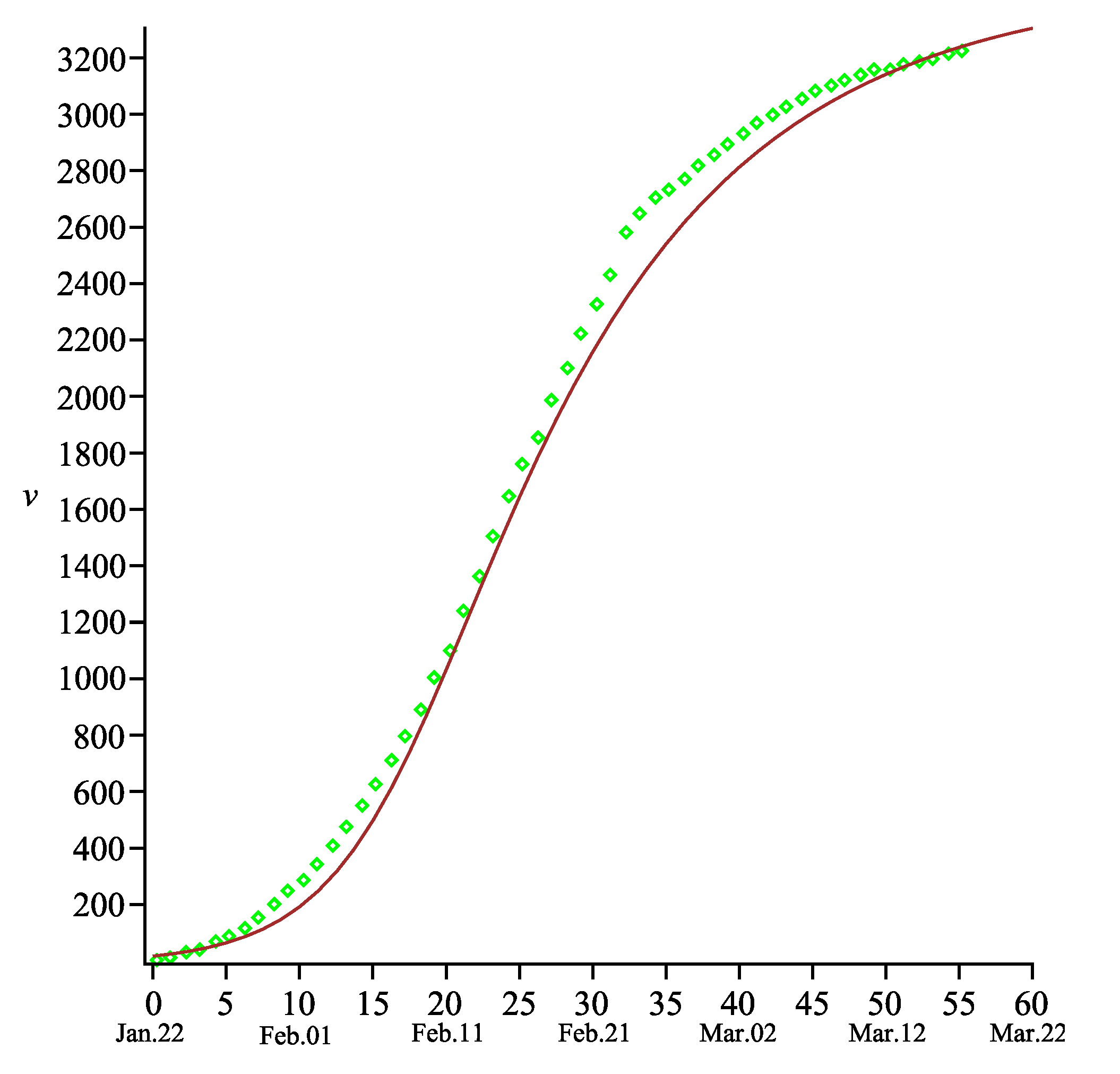
Figure 1 and
Figure 2 present the comparison of the results obtained from the model (
1) and (
3) (with the parameters specified above) and the measured data for the COVID-19 outbreak in China [
9]. One may note that there is a good agreement between the total number of the COVID-19 cases and that predicted by our model. Of course, one may claim that exactness is not sufficiently good in the interval
in
Figure 1. However, we assume that either the method of measurement of the COVID-19 cases was corrected, or an unpredictable spike of such cases occurred around date
(there is a jump from 44,653 cases on 11 February to 58,761 cases on 12 February [
9]).
The comparison between the total number of deaths and that predicted by our model shows that exactness is sufficiently good for any time (see
Figure 2). One may also note that the function
is still increasing beyond the time
. Such behavior reflects the real situation in the epidemic process, namely: some people will die even in absence of new COVID-19 cases because they were infected earlier. Therefore, the final number of total deaths will be fixed later than that of the COVID-19 cases.
It should be noted that the parameter
plays essential role if one uses Equation (
2) instead of Equation (
1). In order to highlight this, we present exact solutions of Equation (
2) with different values of
in
Figure 3 (all other parameters are the same as in
Figure 1). One may see that
is a good choice in the case of China. On the other hand, taking into account the known data [
9], we conclude that
in the case of many other countries (see the next section).
4. Application for the COVID-19 Outbreak in Austria and Poland
In the previous section, the mathematical model proposed was used for quantitative description of the outbreak of novel coronavirus COVID-19 in China. Although the model is relatively simple, the comparison with the data listed in [
9] shows that the analytical solution of the model (with the correctly specified parameters) leads to the results, which are in good agreement with the measured data.
Some well known recommendations naturally follow from the model. It follows from the exact solution (
11) that one needs to reduce the coefficient
as much as possibly. It means that the number of contacts
S should be minimized. On the other hand, the government should make more efforts (to close shops, restaurants, to restrict transport traffic, etc.) in order to increase the function
. These efforts should increase with growing of the total number of the COVID-19 cases. The government restrictions can be partly lifted only under condition that that the number of new COVID-19 cases per day already began to decrease from day to day. It means mathematically that the second order derivative of the function
takes negative values. In order to find the so-called critical number
, we analyze the function
from (
11). Calculating the second order derivative, one obtains
Solving the algebraic equation
with respect to the time, we arrive at
hence
On the other hand, formula
allows finding the parameter
b provided the time
is known from the measured data. Assuming that
a is known one calculates
In the quite similar way, one can obtain the analogous formulae using the exact solution (
12) of the model (
2) and (
3). These formulae have the form
i.e.,
Taking into account interpretation of the parameters, we believe that the parameter
a varies not so much as
b and can be specified (at least estimated with a sufficient exactness) as follows. Obviously, the total number of the COVID-19 cases in the initial period of epidemic process can be approximated as
(see
in (
11) and (
12) for small time). Therefore, having the measured data in the initial period, we may specify the parameter
a. It means that our model allows predicting the total numbers of the COVID-19 cases if the data for
and
are known.
Example 1. Let us consider an example. It can be noted from the public data [9] that the COVID-19 outbreak in Austria had the maximum number of new daily cases on 26 March. Therefore, . If we fix 8 March as the initial point , then and (we think that there are essential errors in measuring at the very beginning of the epidemic process, so that it is unreasonable to start from very small numbers of ). Now we make approximation of the measured COVID-19 cases using the formula
during the first 10 days. It can be estimated that the parameters
provides a good approximation. As follows from the public data [
9], the total number of the COVID-19 cases in Austria reached 15,002 on 23 April (notably we predicted on 8 April, that this number will be 13,800 [
8], i.e., the error is only 8 percent). After this date, the new daily cases numbers are very small (at maximum 0.5 percent of the total number) so that we conclude that the COVID-19 outbreak is over in Austria (of course, some number of infected people will still need medical treatment for several weeks). Therefore, we may define that
15,000. Now we assume that in this case the same model works as for China. Therefore, using Formula (
13) the exact value of the parameters
a and
b were specified and the relevant exact solution for the function
was compared with the public data. The result is presented in
Figure 4 (left) and one realizes that exactness is not acceptable. We conclude that
should be taken in the model.
Assuming
, we have done the analogous calculations using Formula (
14) for different values of
. As a result, the parameter
was found as one of the best choices. The result is presented in
Figure 4 (right) and now one may claim that the exact solution of the model
fits to the real data very good. The total number of deaths
can be also calculated using the second formula in (
12) with correctly specified parameters
and
. The comparison with the measured data is presented in
Figure 5.
Remark 2. It can be checked using the public data [9], that the exponent is common for several countries in Europe. See example, for France in Figure 6. Example 2. Let us consider another example with the aim to make some predictions. It can be noted from the public data [9] that the COVID-19 outbreak in Poland is still dangerous. One may note that the maximum number of new daily cases occurred on 19 April. Therefore, we take . If we fix 14 March as the initial point , then and . There are essential errors in measuring at the very beginning of the epidemic process, so that it is unreasonable to start from very small numbers of . Of course, one may take, say, 12 March or 16 March as , however, it will be shown below that the result will be almost the same. Therefore, making approximation of the measured coronavirus cases using the formula
at the initial stage of the COVID-19 outbreak, the interval for parameter
was identified. Assuming that again
and using the formula (see (
12))
an analog of Formula (
13) can be easily derived. Now we may predict that the total number of the COVID-19 cases in Poland should be
19,700. The relevant exact solution for the function
was compared with the public data and it was noted that a deviation occurs between our exact solution and the measured data.
A better exactness can be reached if one replaces
by
(see
Figure 7). In such case, the total number of the COVID-19 cases in Poland should be
21,000. Notably, if one takes either 12 March or 16 March as
then almost the same curves for
are obtained, while the maximum difference between
is only
percent. It is a good exactness because we estimate the exactness 10 percent in our predictions. Notably, in contrast to Austria and France, the spike of the COVID-19 cases per day in Poland is not so obvious. This is probably a reason the exponent of nonlinearity
is different.
Thus, the total number of the COVID-19 cases in Poland will be about 21,000 (with the above listed exactness). This number will be reached in the middle of June 2020 and only 50–100 COVID-19 cases per day will be identified in the second half of June. Of course, if, for example, the Polish government lifts the restrictions protecting the coronavirus spread too early then can be much higher. Notably, such decision of the Polish government indeed took place when this work was finished. Moreover, a severe COVID-19 outbreack started in the beginning of May 2020 in the region Silesia; probably it is a concequence of weak quarantine restrictions. As a result, our above prediction can be understated because the parameters a and b should be modified.
Finally, it should be noted that Ukraine follows Poland with some time-shift, therefore a similar dynamic of the COVID-19 epidemic process should be expected in Ukraine.
5. Discussion
In this work, we suggested to use the Equations (
2) and (
3) as the mathematical model for describing the COVID-19 epidemic in several countries. Although it is not absolutely new model, one possesses two remarkable properties. Firstly, the model is integrable; secondly, one produces the results, which are relevant to the measured data in several countries. Moreover, it can be done without long and complicated numerical simulations. Notably, we predicted on 8 April using the model, that the number COVID-19 cases in Austria will be 13,800 [
8], i.e., the error was less than 10 percent w.r.t. the measured data in the end of April.
We also developed a generalization of the model in the form (
4)–(
5). It is shown that this model is also exactly solvable and its exact solution is given by the Formula (
8)–(
10). We are going to apply this model to some countries with a hight mortality rate in a forthcoming paper.
Notably the above models imply that the parameters a and b are constant. However, they should depend on time if the government will decide to lift essentially the quarantine restrictions too early (see the above mentioned decision of the Polish government). On the other hand, a mathematical problem arises concerning exact solving the models obtained.
Obviously, the model presented in this work cannot be thought of as applicable for the COVID-19 outbreak in each country. For example, the outbreak in China was mostly localized in the province Hubei. The size and population of this province are very small when compared with the total of those in China. Therefore, the space distribution of the infected population can be neglected. The similar situation is with small countries such as Austria, in which this space distribution is homogeneous by definition, i.e., it is another implication of the models.
On the other hand, if we take the epidemic process in Italy then one notes that the size and population of the most affected part, Northern Italy (eight provinces, Lombardia being largest among them) are comparable with those all of Italy. Therefore, we propose that the space distribution of the infected population should be taken into account in such cases. Moreover, we cannot assume that the model that
in the case of Italy because the total number of deaths cases exceeds 14 percent of the total COVID-19 cases. In such cases, the natural generalization of the basic equations of our model reads as
where
is the Laplace operator,
and
are diffusivities, the functions
and
are analogs of
and
. Of course, the generalized model based on the system (
15) and relevant boundary conditions (for example, zero flux conditions at the boundary) is much more complicated problem and cannot be solved analytically in contrast to the nonlinear models (
2)–(
3) and (
4)–(
5).
In the case of low mortality rate, i.e.,
, the above system simplifies to the form
Here we note that the first equation in (
16) with
is the classical Fisher equation [
20], which was extensively studied in many works (see, e.g., the monographs [
12,
21] and papers cited therein).
Notably, the system (
16) can be essentially simplified under the reasonable assumption
to the form (here
)


