3.1. The Proposed Stock Allocation Method
In consideration of the invisible connection between cognition and price, the cognitive bias needs to be measured if it is applied as criteria for stock allocation. In this section, we first construct a state-space model to describe how cognitive biases play a role in the trading procedure. Then, collective cognitive biases are estimated by incorporating the hybrid algorithm of Kalman filtering and EM (expectation maximization). Finally, with the help of previous estimation, the symmetric investment allocation is accomplished based on the investors’ risk preference.
Step 1. Build a state-space model.
The construction of variables can be found in
Section 2.1. For a better understanding, the concepts of the variables are described in
Table 2.
The state-space model can be expressed as follows:
Equation (12) is the signal equation, and Equation (13) is the state equation. are the known variables; denotes the logarithm of ; and xi (i = 1, 2, 3) represents the cognitive bias induced by factor , which will lead to changes in the trading volume. The value of cognitive bias cannot be observed directly. and are independent Gaussian noise, and their variances are denoted as and , respectively. Parameters of the equation need to be estimated.
By ascribing to the cognitive bias in decision-making, people think they can balance their portfolio in a rational way, whereas they cannot. The brain mechanism always leads people to make similar cognitive choices when facing information stimuli. These similar decisions push the trading volume away from average so that stock prices are changed, which is reflected in Equation (12). Besides, habitual thinking can also have an impact on existing cognition, which is reflected in Equation (13). Therefore, we are convinced that it is feasible to denote cognitive bias in the form of “trading elasticity” (i.e., the sensitivity of the trading volume to a specific information stimulus).
Step 2. Kalman filtering.
In addition to measuring the unobservable value (the value of at time t), the application of the hybrid algorithm can better reflect the interaction effect between parameters and variables. The initial setting on estimation can be acquired by the Monte Carlo stochastic points method. In the first round of iteration, we used Kalman filtering to estimate .
The conditional distribution mean of
is the unbiased estimator under the minimum mean square error, which is performed as follows:
The covariance of the corresponding estimate error can be expressed in the form:
where
is denoted in Equation (17):
can be corrected once
is obtained, and the modified equation is constructed as:
where
is represented as below:
The expression of
can be given in the same way:
Based on the output
and
, the backward recursion starts from
to
, which is represented as:
where
. The first unbiased estimation of
is acquired via iteration.
Step 3. EM algorithm.
Before the EM algorithm, the joint probability density of
and VR need to be derived:
Due to the invisibility of variable
, the likelihood function cannot realize maximization. If it does apply in the algorithm as a need, it is required to get the conditional expectation in logarithmic form, which is called the E-step. For reasons of space, the conditional expectation omits the conditional representation in the process:
We can obtain the partial derivative of every parameter as above, targeting the maximum conditional expectation. This process is called the M-step. After transformation, the explicit expression for the parameter is as follows:
These expressions and the output in step 3 can be combined to find the unbiased parameter estimates via the second round of iteration.
Step 4. Multiple iteration until convergence.
By using Kalman filtering and the EM algorithm alternately, these parameters and the variable are continually put into the cyclic iterations and constantly updated, until the convergence of the conditional likelihood function. After rounds of iteration, we finally gain three kinds of cognitive biases, which are denoted as , and .
Step 5. Calculate EMACB (exponential moving average of cognitive bias).
First, we tried to calculate the 12-day EMACB, which denotes the slow-trend moving average of cognitive bias:
where
means the value of the
ith cognitive bias of a portfolio, and
denotes the weight of the
kth stock in the portfolio.
Then, the 5-day EMACB is chosen to be calculated, which denotes the fast-trend moving average of cognitive bias:
Step 6. Make the EMACB-variance model (EV Model) for risk seekers to obtain the optimal weights of each stock.
As risk seekers, they would rather take more attention on how to acquire higher compensation for risk, rather than focus on the potential possibility of loss. Based on this, the optimal decision can be constructed as follows:
where
denote the price of stock
m and stock
. Under the limited risk, the gap between two EMACB indicates the changing trend of cognitive biases. It reveals the deviation from traders’ price expectation to real value. Additionally, this kind of deviation will increase the possibility of a price rebound, which is similar to the momentum reversal principle. Therefore, the trend gap can be regarded as the effective signal of prospective return.
Step 7. Make the EMACB-variance model (EV model) for risk averters to obtain optimal weights of each stock.
As a risk aversion decision-maker, they would like to get steady returns with minimum risk. Based on this, the optimal decision can be constructed as follows:
3.2. Illustrative Example for Stock Allocation
In order to get heterogenous decisions based on symmetric risk preference, we would like to give an example to illustrate the application of the proposed method for stock allocation.
A stock agent from a security company in Guizhou, China intends to make investment plans for two clients with different preferences. The plans aim at optimizing the portfolio allocation in September, 2019. Through risk assessment tests, the results indicate that one of the two clients is a risk seeker while the other one is a risk averter. The stock agent decides to pick stock
as the alternative stocks in portfolios. Considering the correlated risks, the chosen stocks come from different industry segments (i.e., precision instruments, liquor, virtual game, chip and biomedical treatment). The specific descriptive statistics of the stocks can be found in
Table 3. Meanwhile,
Table 4 shows that there is no significant correlation between any two stocks at the 95% confidence level. In view of differential risk appetites, the agent suggests the risk seeker invests 70% of funds in the stocks while the risk averter 30%. The stock portfolio allocation procedure is shown as follows.
For measuring collective cognitive bias in the chosen stocks’ price, the agent firstly collects data from September, 2010 to August, 2019. A few missing values in this period can be filled by multiple imputation with a mice package in R language; in other words, we can estimate the conditional probability of the missing value by using the existing data to complete the filling work.
Then, with the collected data, the process of stock allocation based on the measurement of cognitive bias is presented as follows.
Step 1. Before measuring, the ADF test needs to be used to recognize whether each time series participated in construction is a stationary sequence, including the series of the volume ratio (VR) and the logarithmic forms of
, which are defined in
Table 1 and
Table 2. the results are shown in
Table 5.
Step 2. to avoid false regression, these variables need to be tested by the Johansen co-integration test, which concludes the trace test and maximum characteristic value test. The results are shown in
Table 6.
Step 3. Construct the state-space model based on collected data.
Step 4. Estimate cognitive bias using Kalman filtering.
Step 5. Modify the coefficients’ estimation generated in step 4 by the EM algorithm.
Step 6. Put the revised estimation into Kalman Filtering to continue the next round of iteration, until convergence. Based on the results, some features of cognitive biases are shown in
Figure 1,
Figure 2 and
Figure 3. Additionally, the estimation results are shown as follows:
Step 7. Calculate the 5-day and 12-day EMACB based on the previous measurement outcomes.
Step 8. Construct the EV model for the risk seeker and calculate the objective weights of each stock.
Step 9. Construct the EV model for the risk averter and obtain the weights allocation. The results of step 8 and 9 are expressed in
Table 7.
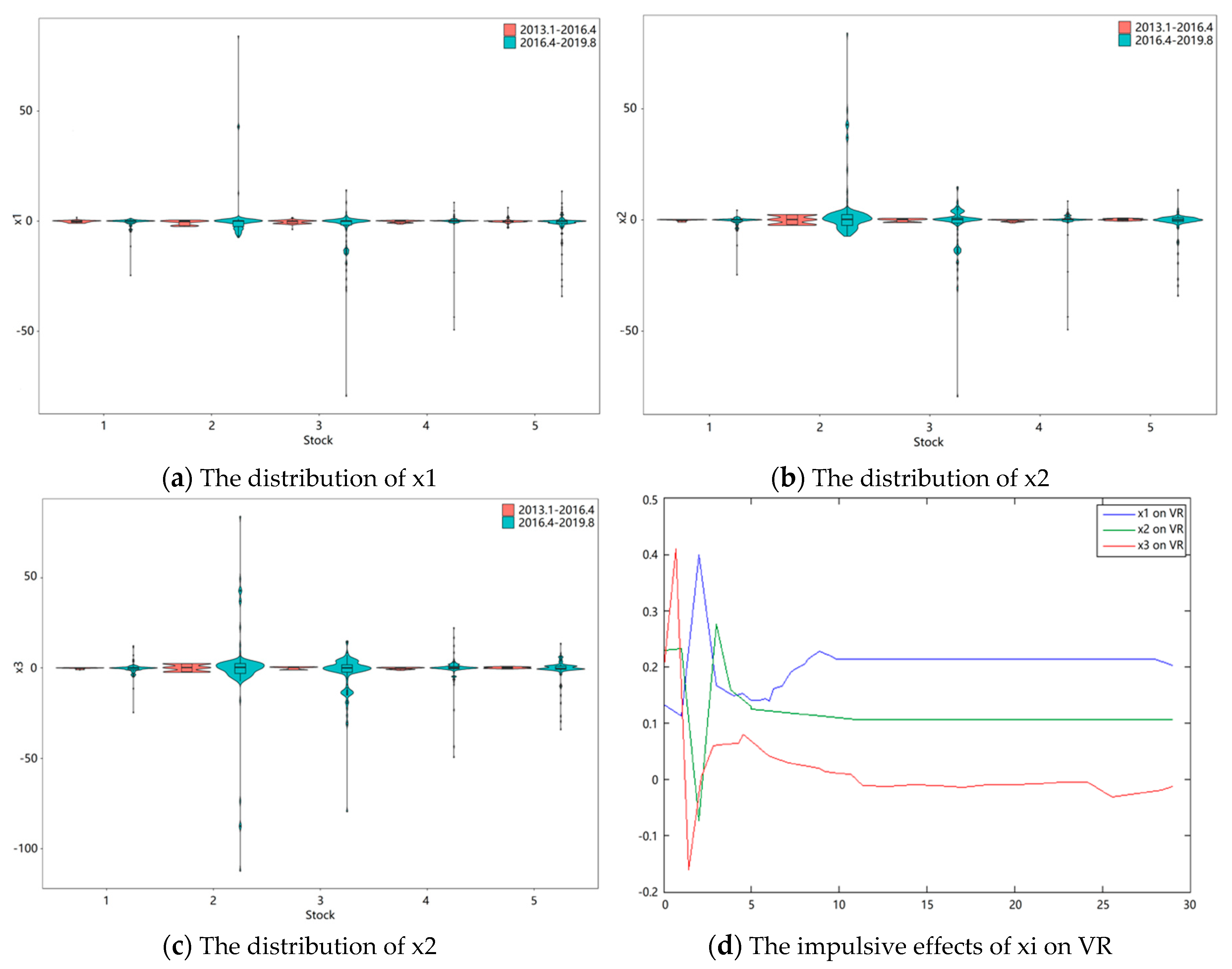
Figure 1a–c reveal the distributions of the chosen stocks’ collective cognitive bias (x1, x2, x3). These distributions are acquired by a series of data that originated from two periods. What can be found in the figures is that the possible value range of three cognitive biases in the second time period are much broader than the first period. The features shown in the picture support the fact that the increasing volume of information in the economic environment does interfere with judgment, and leads to more severe cognition bias.
In
Figure 1d, the stock trading volume ratio varies with the changes of the cognitive bias in a short period. Sudden changes in cognitive bias can lead to violent trading swings. In the long run, the equilibrium price is determined by the asset value, which is not affected by short-term cognition. Besides, the red curve has the strongest impulsive effects among the three curves, which indicates the VR (volume ratio) is more sensitive to anchoring values.
It is obvious in
Table 7 that the risk averter tends to give more evenly weights for each chosen stock, which is different from the risk seeker. In other words, the risk averter has stronger demand to diversify risk in the investment prediction of September, 2019. However, the results only represent the investment features in one month with a 5-stock portfolio. Whether the proposed method has value in general applications still need to be verified in
Section 4.


