Article

A New Objective Function for the Recovery of Gielis Curves

by
Alejandro Marcelo Arce
1,†,
Gabriel Giovanni Caroni
1,†,
José Luis Vázquez Noguera
1,*,†,
Diego P. Pinto-Roa
1,†,
Horacio Legal-Ayala
1,† and
Sebastián A. Grillo
2,†
1
Facultad Politécnica, Universidad Nacional de Asunción, San Lorenzo 2160, Paraguay
2
Faculty of Science and Technology, Universidad Autonoma de Asunción, Asunción 1255, Paraguay
*
Author to whom correspondence should be addressed.
These authors contributed equally to this work.
Symmetry 2020, 12(6), 1016; https://doi.org/10.3390/sym12061016
Submission received: 26 March 2020 / Revised: 29 May 2020 / Accepted: 3 June 2020 / Published: 16 June 2020

Abstract

:
The superformula generates curves called Gielis curves, which depend on a small number of input parameters. Recovering parameters generating a curve that adapts to a set of points is a non-trivial task, thus methods to accomplish it are still being developed. These curves can represent a great variety of forms, such as living organisms, objects and geometric shapes. In this work we propose a method that uses a genetic algorithm to minimize a combination of three objectives functions: Euclidean distances from the sample points to the curve, from the curve to the sample points and the curve length. Curves generated with the parameters obtained by this method adjust better to real curves in relation to the state of art, according to observational and numeric comparisons.

1. Introduction

The importance of detecting and representing shapes is recognized by several research communities such as engineering [1,2] and computer science community [3]. In [2], superquadric shapes (such as cuboids and lozenges) have been numerically studied. Gielis curves can describe shapes of nature and shapes made by man, including geometric figures [4]. This makes its use possible in areas such as botany and it is even used for road signal recognition [5]. In other works [6,7], an infinite plasmonic cylinder (whose cross-section is described by the Gielis superformula) is optimized.
Duda and Hart defined pattern recognition as “the field concerned with machine recognition of meaning regularities in noisy of complex environments” [8], this includes shape recovery. One of the most common ways to represent shapes is with the use of superquadrics [9,10]. Superellipses represent shapes of two dimensions, but they have the disadvantage of limited symmetry. Shapes represented by superellipses necessarily have two symmetry axis, i.e., four sections. As a result of this, many shapes of nature and objects can not be represented with them.
With the aim to overcome the mentioned inconveniences, Johan Gielis proposed the superformula [4] that generates curves called Gielis curves. The superformula allows obtaining a greater degree of freedom, being able to represent organisms of nature, objects and geometric figures using a small amount of input parameters. In exchange for getting a greater degree of freedom, it is more difficult to perform the shape recovery.
Gielis curves can be classified as self-intersecting and non-self-intersecting. Fougerolle et al. [11] and Gielis et al. [12] proposed methods for the recovery of Gielis curves from a set of sample points. Some experiments on fitting of Gielis curves by simulated annealing and particle swarm methods of global optimization were made by Sudhanshu K. Mishra [13].
We propose a new objective function based on the method proposed by Fougerolle et al. [11], focusing on non-self-intersecting Gielis curves, without noise and without translation or rotation, minimizing a function that combines the distance from the sample points to the curve, the distance from the sample points to points of the generated curve and the curve’s total length. In addition to visual evaluation, we propose a metric for numeric comparison of the obtained results.
The rest of the paper is divided as follows: in Section 2, Gielis curves are presented, that are calculated using the superformula, which is a generalization of the superellipse [4]. In Section 3, the background to the problem is presented. Then, in Section 4, the proposed method is presented. Experiments and obtained results are presented in Section 5 and conclusions and future work in Section 6.

2. Gielis Curves

As mentioned before, Gielis curves are introduced for representing shapes with variable symmetry such as those in nature and objects. Gielis curves are a generalization of the superellipses, which are defined by the formula:
x a n + y b n = 1 ,
where x is the axis of abscissas, y is the axis of ordinates, a R + is the maximum value of x, b R + is the maximum value of y and n R + 0 define the shape of the curve.
Standard ellipses can be generated with n = 2 . For n < 2 , curves are inscribed in that ellipse, i.e., they fit inside it, and the curve is called hypoellipse. For n > 2 , curves are circumscribed about that ellipse, i.e., that ellipse fits inside the curve, and the curve is called hyperellipse. In the limit case where n is infinite, a rectangle is obtained [14]. Figure 1 shows examples of superellipses. The first one is a hyperellipse, the second one is a circumference and the third one is a hypoellipse.
Specific rotational symmetries are introduced with the use of polar coordinates ρ = f ( θ ) , where ρ is the distance to the origin or pole and θ is the angle that forms with the polar axis, equivalent to the x axis in the cartesian system; and adding the argument m 4 to the θ angle. In addition, exponents n 1 , n 2 and n 3 are introduced, replacing exponent n used in Equation (1). This leads to the function in Equation (2), which is called superformula [4]:
ρ ( θ ) = 1 1 a cos ( m θ 4 ) n 2 + 1 b sin ( m θ 4 ) n 3 n 1 ,
where m R + 0 is the value of rotational symmetry; a R + is the maximum length in the polar axis; b R + is the maximum length in the perpendicular to the polar axis and n 1 , n 2 , n 3 R + 0 determine the shape of the Gielis curve.
The argument m indicates the amount of points that are fixated in the ellipse of semi axis a and b, that is centered in the origin of coordinates. As occurs with superellipses, for n 2 = n 3 < 2 the Gielis curve is inscribed in that ellipse, and for n 2 = n 3 > 2 the Gielis curve is circumscribed about that ellipse. Original superellipses, given by Equation (1), can be generated by Equation (2).
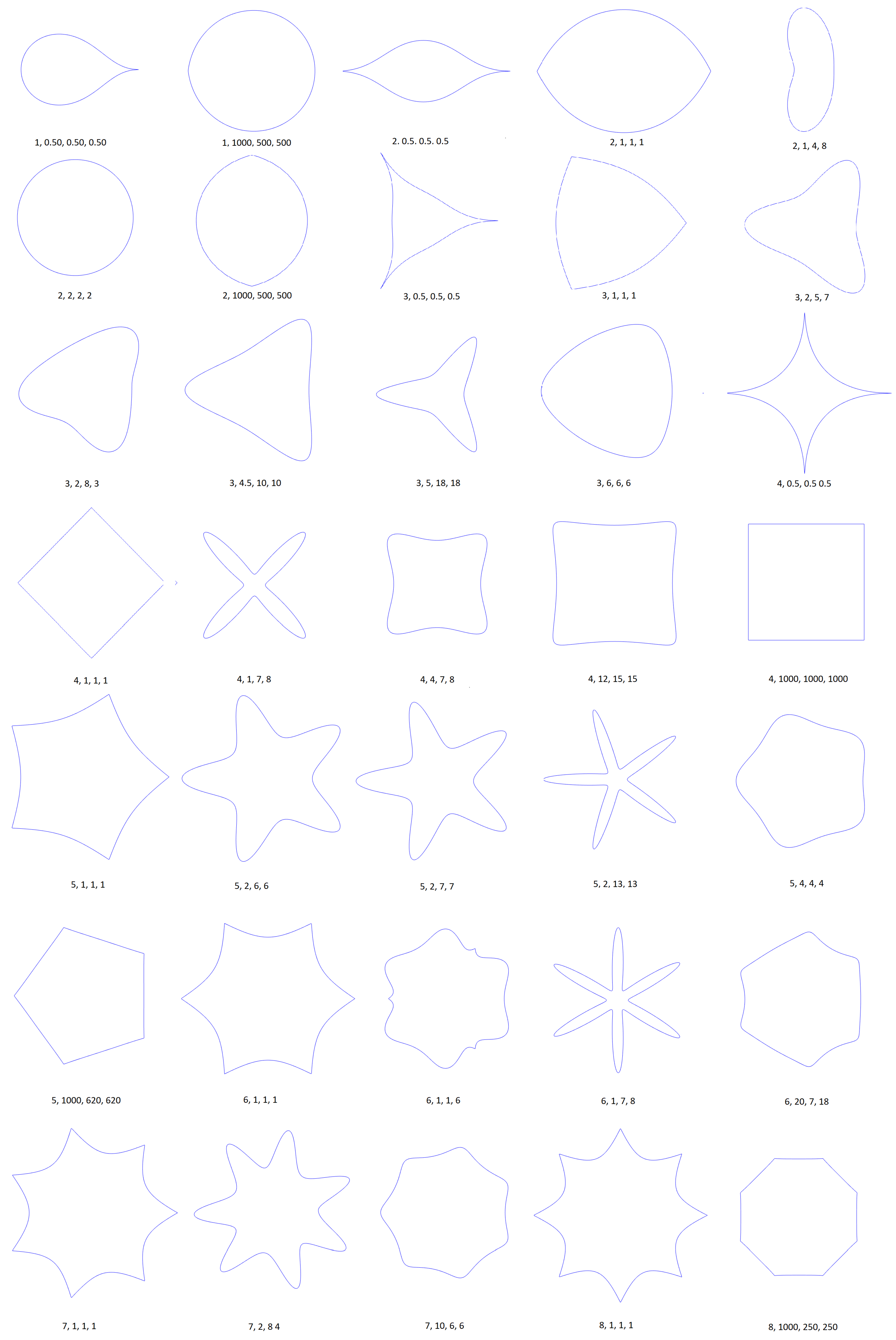
We may find complex shapes that are very different to view, but that have in common the property of being able to be represented by the superformula. These shapes can be organisms, objects and geometric figures. Figure 2 shows examples of Gielis curves generated by Equation (2) that can not be represented using Equation (1).
Parameter m can be viewed as p/q, where p N + 0 is the number of sectors of the Gielis curve (symmetry) and q R + 0 is the maximum number of intersections of the Gielis curve with itself, where p and q are relative primes [11]. The generated Gielis curve is repeated every 2 π for integer values of m and every 2 q π for rational values of m, i.e., only data generated by the function (2) within the [ 0 , 2 q π ] interval is analyzed.
Unfortunately, methods for recovery of superllipses are not directly applicable to Gielis curves [11]. For this reason, effective methods to perform recovery of Gielis curves are still developed. This recovery can be viewed as a optimization problem, where from sample points we minimize some objective functions under certain restrictions.
Optimization problems can be solved with the use of deterministic and stochastic algorithms. Deterministic algorithms follow a rigorous process and their execution is reproducible, with the risk of falling into local minima when the problem structure is non-convex. To overcome this drawback, stochastic algorithms always have some degree of randomness [15]. Genetic algorithms are inspired on the evolution of populations and they provide a natural and intrinsic way to explore the solution space [16,17]. Each individual in the population represents a problem solution. Selection and recombination are genetic operators performed on the current population to generate a new promising population. To avoid premature stagnation, mutation operators inject new genetic information into the population. The development of promising genetic strategies to achieve balance between exploitation and exploration in the solution space has led to the successful application of modern genetic algorithms in several highly complex problems [18,19]. In the next section the application of this type of algorithm for solution searching is presented.

3. Background

In this section we present evolutionary algorithms and the method proposed in [11] for the recovery of Gielis curves from a set of points. This method is based on the algorithm proposed by Bokhabrine et al. [20].
Evolutionary algorithms are stochastic search methods, inspired by biologic evolution, and they have been applied successfully in several pattern recognition problems [21,22,23]. Each individual from the population represents a solution, and each individual has an associated fitness that measures its adaptation to the environment, i.e., the quality of the solution. Individuals are composed by a set of variables, called genes. Operators applied in evolutionary algorithms are based on mechanisms of biological evolution, such as selection, mating or crossover and mutation. The selection process is the one that determines which individuals will be used to create new generations, i.e., perform crossover. The crossover operator is applied between the selected individuals, the parents. This operator produces descent individuals, that are obtained by the combination of the genes from the parents. The mutation operator produces random changes in the individuals, aiming to achieve greater exploration of the solution space and avoid local convergences, which are the main inconvenient of deterministic algorithms. The mutation rate is a value that must be chosen carefully, since a low value can cause the algorithm to converge to local minima, while a high value can cause the algorithm to behave similar to a random search [11].
Fougerolle et al. [11] proposed a method for the recovery of Gielis curves, using a genetic algorithm as follows:
  • Each gene represents a parameter from the superformula, i.e., each gene may be represented by a real number, except p and q, which are restricted to integer numbers.
  • Crossover is performed as follows: given two parent solutions, two children solutions are obtained, where each child inherits each gene from one of the parents with a probability of 0.5, using a α value between 0 and 1. Since p and q must be relative primes, in case they are taken from different parents, the fulfillment of this condition is verified. If it is not fulfilled, both genes are taken from the same parent, in order for this condition to be fulfilled. Figure 3 shows crossover method: in Figure 3a an example in which the crossover produces a child in which p and q are not relative primes (4 and 2, respectively), and in Figure 3b the correction applied in order for the condition to be fulfilled.
  • In order to perform mutation on continuous variables (a, b, n 1 , n 2 , n 3 ), a normal distribution is used as follows:
    g m u t = N ( g i , k × s i ) ,
    where N is the normal distribution, g i is gene i, s i is the interval length of the variable represented by gene g i and k is a user defined parameter, the suggested value is (0.1). Then, mutation is performed with a normal distribution with a standard deviation of a tenth of the interval length of the variable.
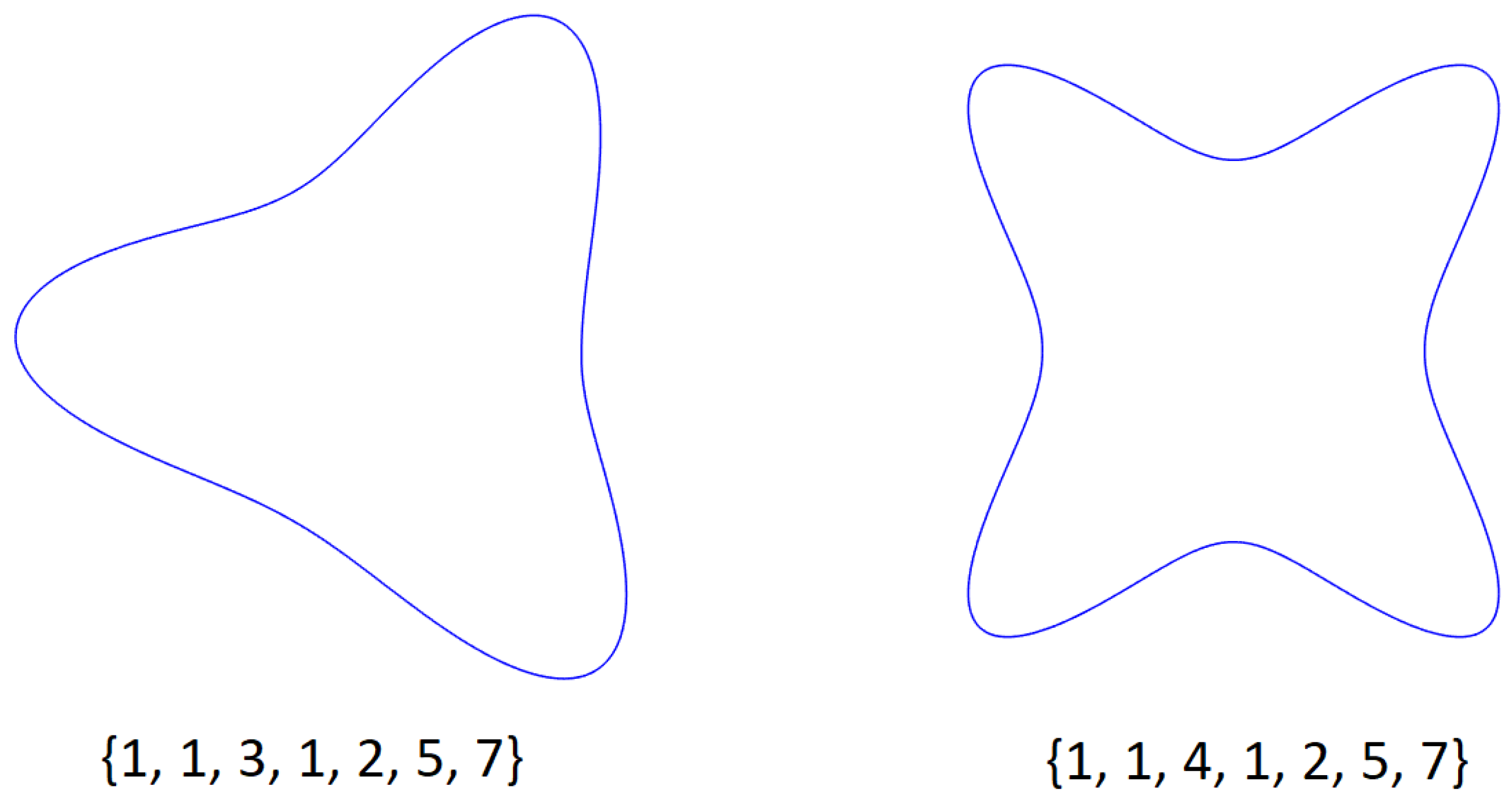
  • Discrete variables (p and q in this case) indicate the number of sectors of the Gielis curve and the maximum number of self-intersections, respectively. When performing mutation, small variations of these variables have no reason for being, since they produce big changes in the adaptation to the sample points. This can be observed in Figure 4, where both Gielis curves have the same parameters, except p, but they have completely different shapes. For this reason, it is suggested to simply generate random values, with the condition that p and q must be relative prime.
  • The selection process is performed as follows: the size of the population is kept constant and individuals with best adaptive value remain. In order to face local convergence and premature convergence issues, Fougerolle et al. [11] suggested to measure the standard deviation of the population after each iteration, and if it is less than a user defined threshold, σ m i n , the population is re-initialized randomly. This is computed with normalized values. The norm used is defined according to Equation (4), denoted as
    v = c c m i n c m a x c m i n ,
    where c F is the value of the variable to be normalized, F = {a, b, p, q, n 1 , n 2 , n 3 } is the set of parameters from the superformula, c m i n is the lower limit of the interval of the variable, c m a x is the upper limit of the interval of the variable and v is the normalized value.
  • If the standard deviation of all variables is less than the defined threshold, population is re-initialized randomly.
The behavior of the population is as follows: as the generation number increases, average error of the population decreases, despite that there can be small perturbations due to the mutation operator, crossover operator is dominant. Once the population converges (the standard deviation is less than the defined threshold), the best solution from the population is stored if this solution is better than the current “global best”, and a random re-initialization of the population is performed, i.e., the best solution so far is always stored, independently from the re-initializations performed. We explore the solution space by this procedure, without losing the best solution obtained so far.
Tests are performed to determine the impact from the mutation and crossover operators using two strategies: the first strategy was to modify the mutation parameter k, the mutation rate and the standard deviation threshold for population re-initialization; and increasing the number of iterations for greater exploration. Applying this strategy, the standard deviation of the population is high and the algorithm does not converge. The second strategy consists in increasing the size of the population by 10, 50 and 100 times. The results are similar, so the conclusion is that performing re-initialization of a small population is more effective than trying to perform a search around local minima or handle big populations [11].
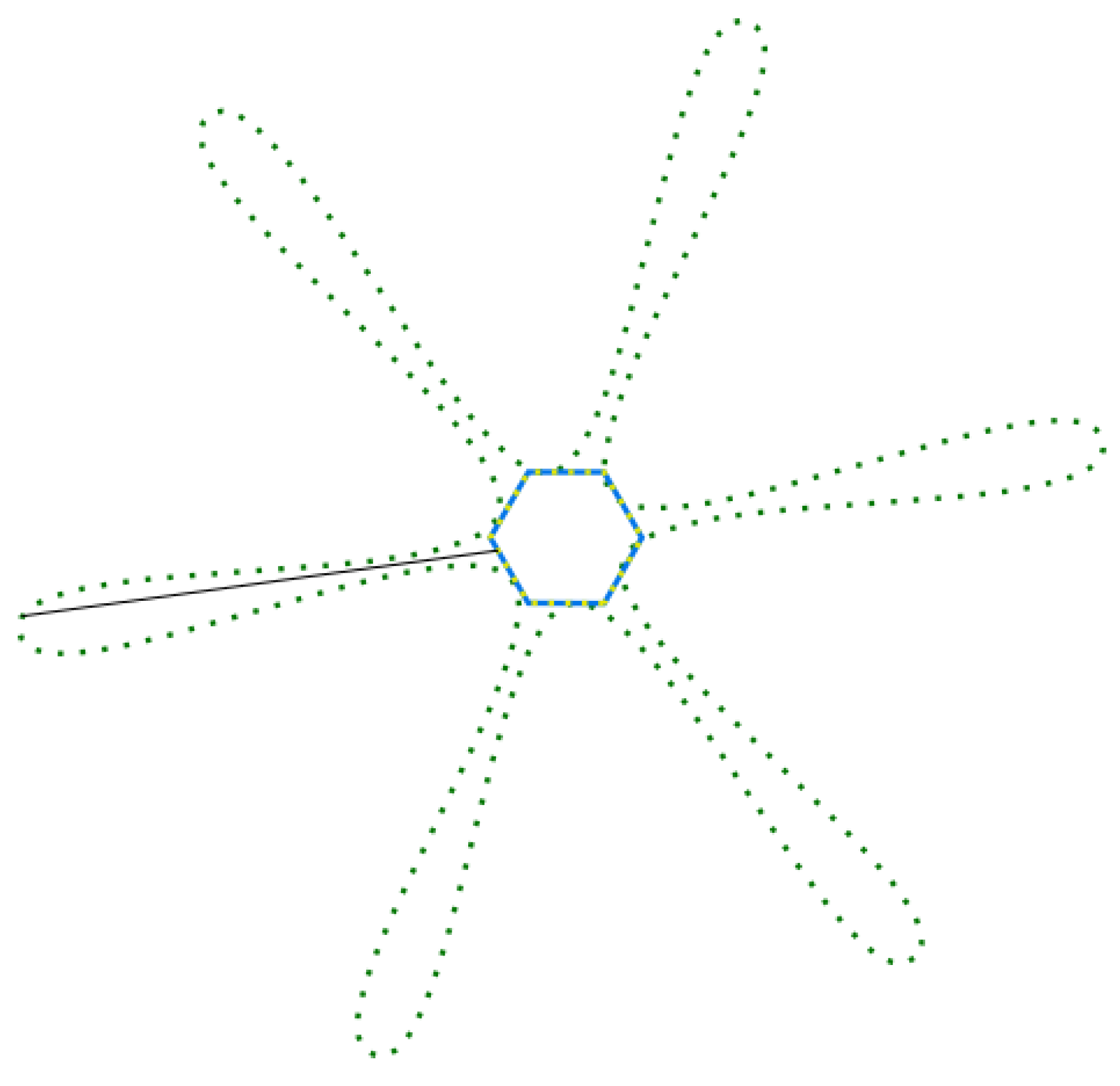
In order to determine the inclusion of a point in respect to a given curve, the use of Shortest Euclidean Distance (SED) between the sample points and the curve is suggested by Fougerolle et al. [11]. Figure 5 shows an example of this SED. In order to compute the SED, sample points from the curve are obtained; then for each point, it is selected the point from the curve with minimum distance. This is given by Equation (5), denoted as
S E D ( Q , F ) = m i n ( d ( Q , R i ) ) ,
where Q = ( ρ , θ ) is a sample point in polar coordinates, where ρ is the distance to the origin and θ is the angle formed with the polar axis, F = [a, b, p, q, n 1 , n 2 , n 3 ] is the set of parameters from the superformula, R i = ( t , ω ) is each one of the sample points from the curve generated with F, in polar coordinates, where t is the distance to the origin and ω is the angle formed with the polar axis and i 1 , 2 , , r , where r is the amount of sample points from the Gielis curve generated with F and d is the Euclidean distance between two points.
Using the S E D , we define an objective function to be minimized, as observed in Equation (6); denoted as
f 1 ( P , F ) = j = 1 e S E D 2 ( P j , F ) ,
where P j is each one of the sample points and e is the amount of sample points.
The function given by Equation (6) is not good enough for obtaining satisfactory results [11]. An example can be seen in Figure 6, where the generated Gielis curve has segments that approach the original curve. The generated Gielis curve also has segments that self-intersect and do not correspond to the original curve.
Fougerolle et al. [11] suggested to also minimize the length of the generated Gielis curve, given by Equation (7), denoted as
l ( F ) = 0 2 q π ρ ( θ ) 2 + d ρ ( θ ) d θ 2 d θ ,
where [ 0 , 2 q π ] is the interval of ρ ( θ ) , ρ ( θ ) is the Gielis curve and d ρ ( θ ) d θ is the derivative of ρ ( θ ) .
In this work, the approximate length of the Gielis curve is calculated easily, dividing the Gielis curve in small sections and computing the distance between the start and finish points of each sections. The calculation uses polar coordinates and sums the computed distances to obtain a total length according to function (8); denoted as
l ( F ) f 2 ( F ) = i = 1 o 1 ρ i 2 + ρ i + 1 2 2 ρ i ρ i + 1 cos ( θ i + 1 θ i ) ,
where ( ρ i , θ i ) , ( ρ i + 1 , θ i + 1 ) , the points between distances, are calculated and o is the amount of points used for computing distances.
Then, the function from Equation (8) is combined with the function from Equation (6) using an R-function. An R-function, proposed by V.L. Rvachev [24], is a real function distinguished because one of its properties is fully determined by that same property of its arguments. For example, the sign of a real function is fully determined by the sign of its arguments [25,26]. In Table 1 possible signs of the function f ( x , y ) = x + y + x 2 + y 2 , are in function of the sign of its arguments. This function is the analytical equivalent to boolean union, considering negative values as false, and positive values as true [25]. On the contrary, f 1 ( x , y ) = x + y is not an R-function since its sign depends on the magnitude of its parameters and not just its signs.
Once the combination of Equations (6) and (8) is performed using the mentioned R-function, the objective function from equation [11] is obtained
F 1 ( P , F ) = f 1 ( P , F ) + f 2 ( F ) + f 1 2 ( P , F ) + f 2 2 ( F ) .
Even with the use of this objective function there are conflictive cases, as can be observed on Figure 7, in which the original curve is not self-intersecting, but the recovered Gielis curve is. Aiming to overcome these drawbacks, this work proposes a variation of the objective function given by Equation (9), which will be explained in the next section. We also propose a numerical evaluation for comparing different methods. Such evaluation complements visual comparison, which will be explained in Section 5.

4. Proposal

This work aims to improve the limits of the objective function in Equation (9) introduced in the previous section.
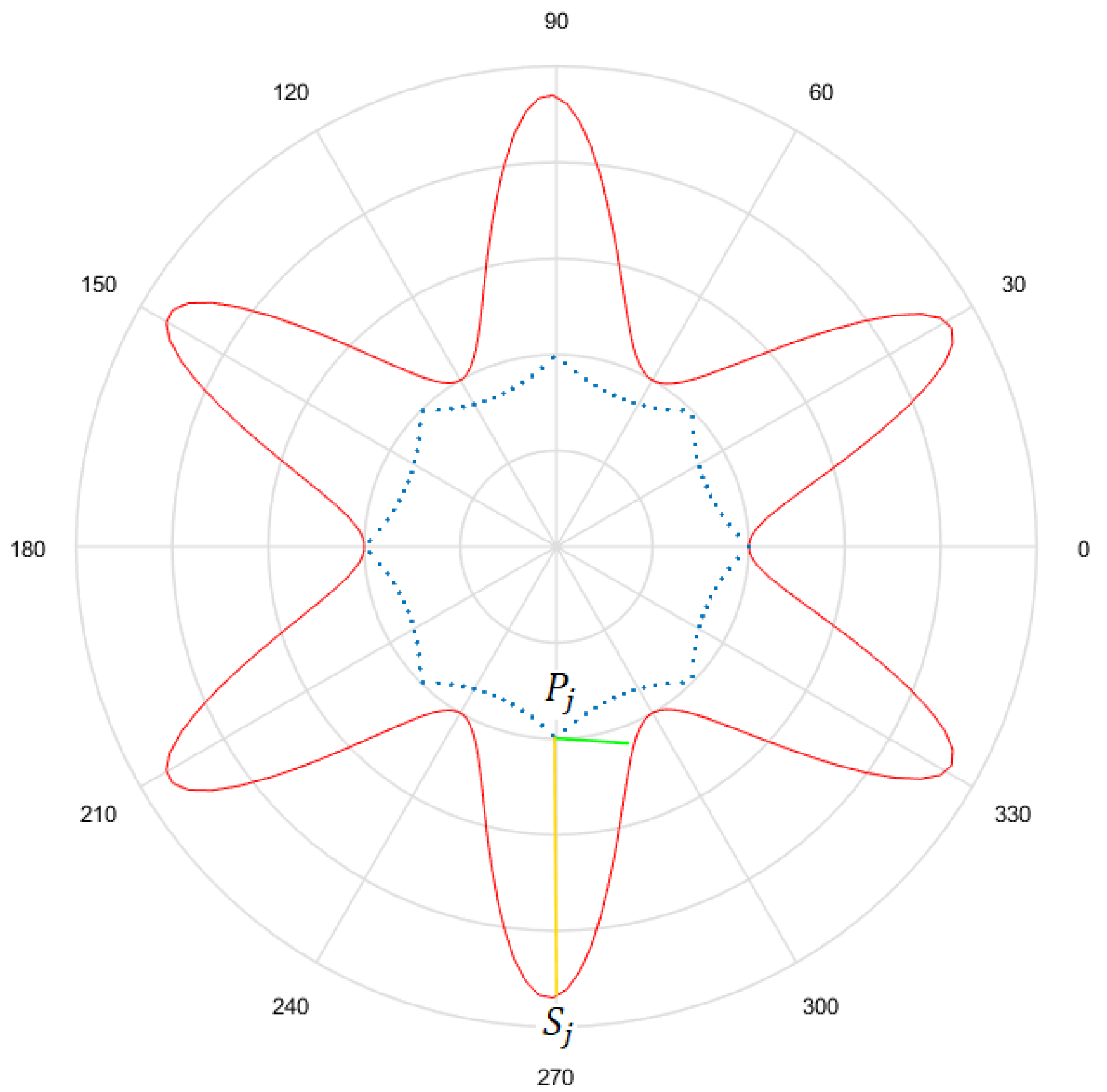
The SED seeks points from the generated Gielis curve, such that they are close to sample points. Therefore we propose a similar metric with the same goal, but with less computational cost. This metric consists in computing the Euclidean distance d( P j , S j ) between the sample point P j = ( ρ j , θ j ) and the resulting point from the generated Gielis curve S j = ( τ j , θ j ) on angle θ j , instead of computing SED. The inclusion of the point to the original curve is still evaluated, but avoiding the iterative method for computing the SED, since the suggested distance is computed directly.
Figure 8 shows the difference between SED and d( P j , S j ). In this case d( P j , S j ) measures differently the approximation of the Gielis curve to the sample points. SED can be in any direction but d( P j , S j ) is always in the same direction than the line between P j and the polar axis.
SED can be replaced by the distance in Equation (6), obtaining
f 3 ( P , S ) = j = 1 e d 2 ( P j , S j ) ,
where P is the set of sample points, S is the set of sample points from the generated Gielis curve, e is the amount of sample points and d is the Euclidean distance.
The length of the Gielis curve is not related to the sample points, as observed in Equations (7) and (8), whose input parameters are solely the superformula parameters and not the sample points. As we need a metric that penalizes the segments from the generated Gielis curve that are far from the sample points, we suggest a new metric instead of the length. The computing of this metric is as follows:
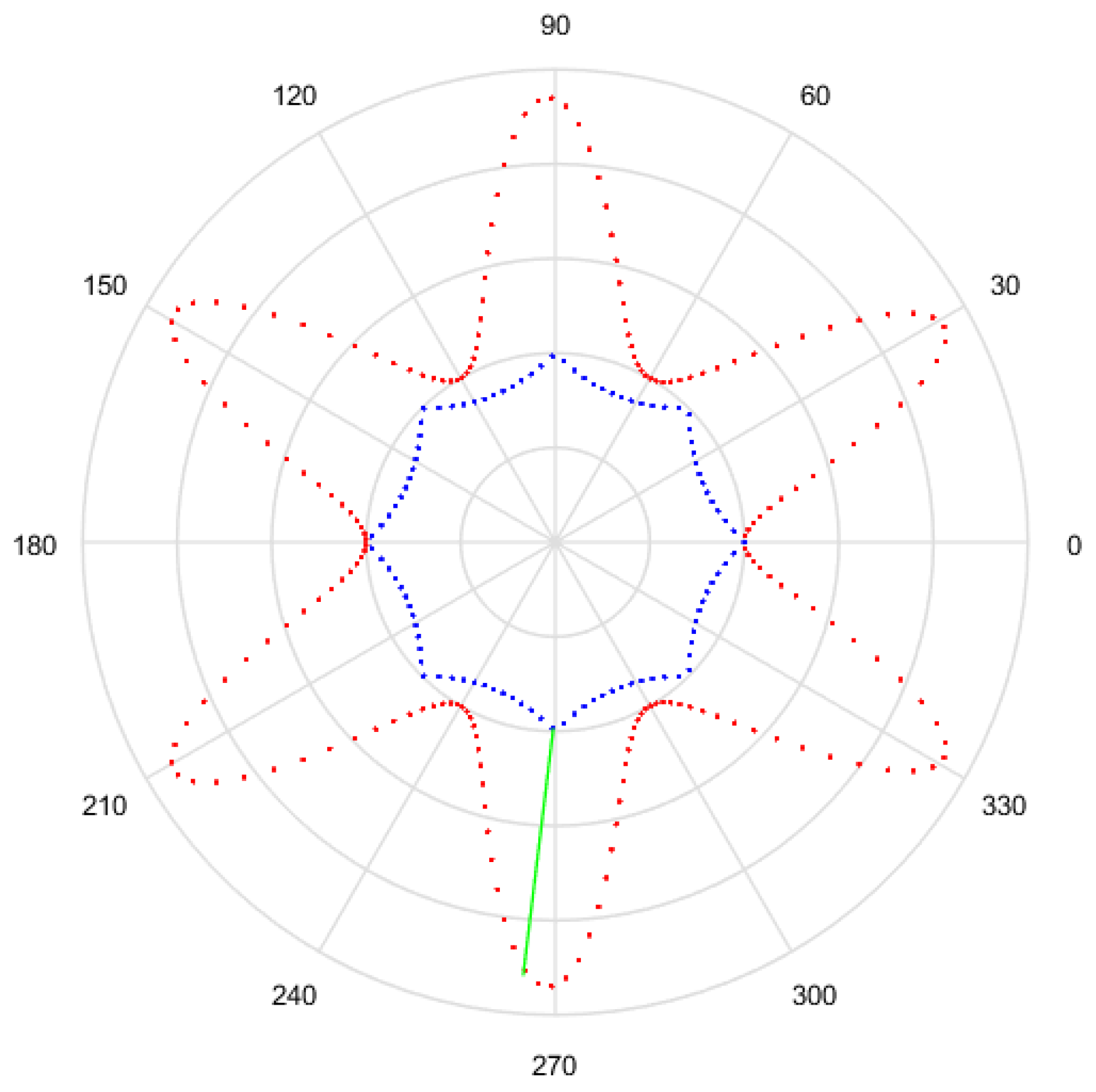
  • Obtain a finite amount of points from the generated Gielis curve, to equals intervals of θ , with a sampling. An example of this is observed in Figure 9, with the points in red.
  • For each point R i = ( r i , ω i ) find the sample point that is closest and compute its Euclidean distance. This distance is observed in green in Figure 9.
The new distance will be called d 2 and is given by Equation (11), denoted as
d 2 ( R i , P ) = m i n ( d ( R i , P ) ) ,
where R i = ( r i , ω i ) is a sample point from the generated Gielis curve, P is the set of sample points and d is the Euclidean distance between two points. Figure 9 shows an example of d 2 and we observe that d 2 penalizes points from the generated Gielis curve that are distant from the sample points.
The function from Equation (12) is built with the sum of squares of d 2 :
f 4 ( R , P ) = i = 1 r d 2 i 2 ( R i , P ) ,
where R is the set of sample points from the generated Gielis curve and r is the cardinality of R.
In order to combine functions from Equations (10) and (12), we use the same R-function than in function from Equation (9). Then, we obtain the following objective function to be minimized:
F 2 ( P , F ) = f 3 ( S , P ) + f 4 ( R , P ) + f 3 2 ( P , S ) + f 4 2 ( R , P ) ,
where S and R are sets of sample points from the Gielis curve generated with F.
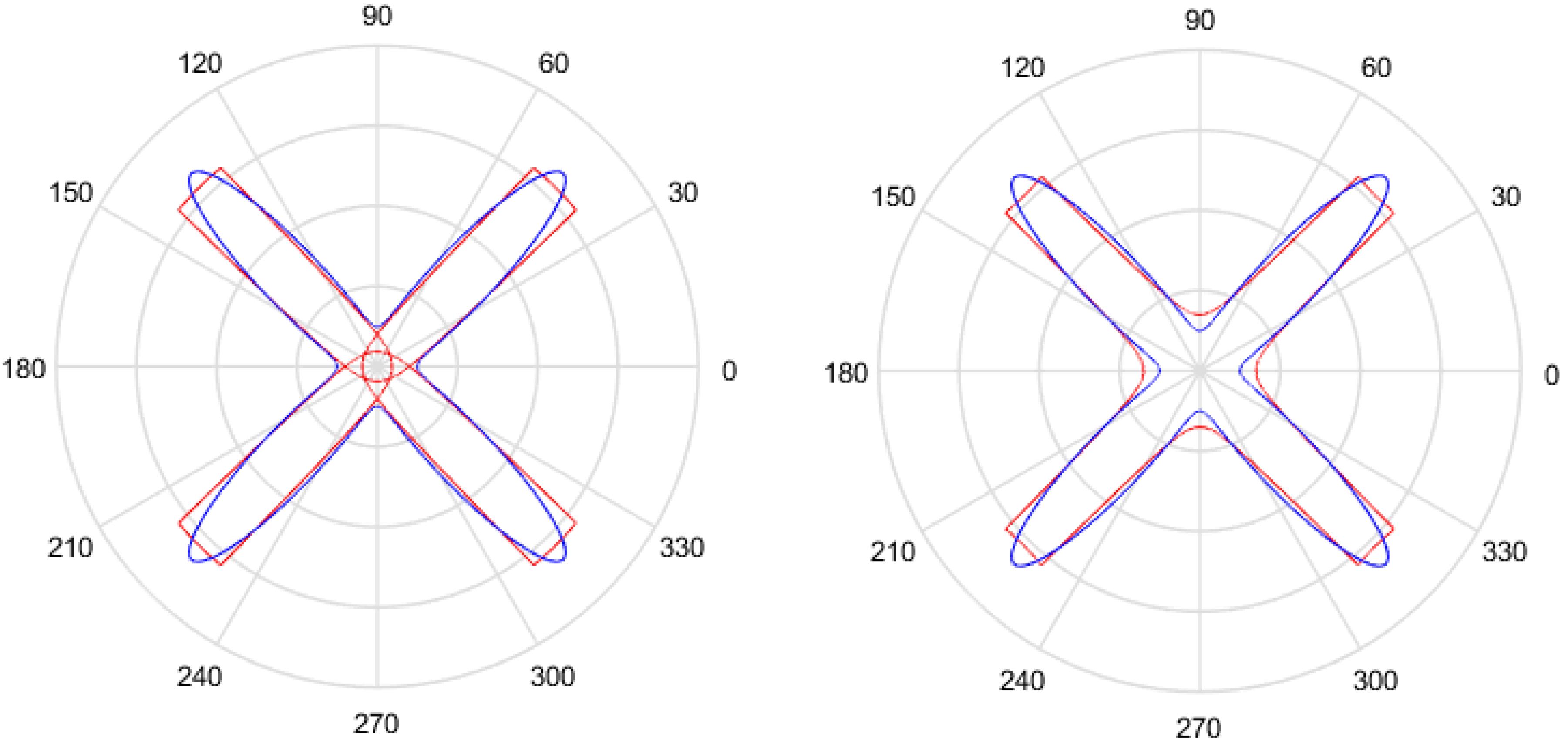
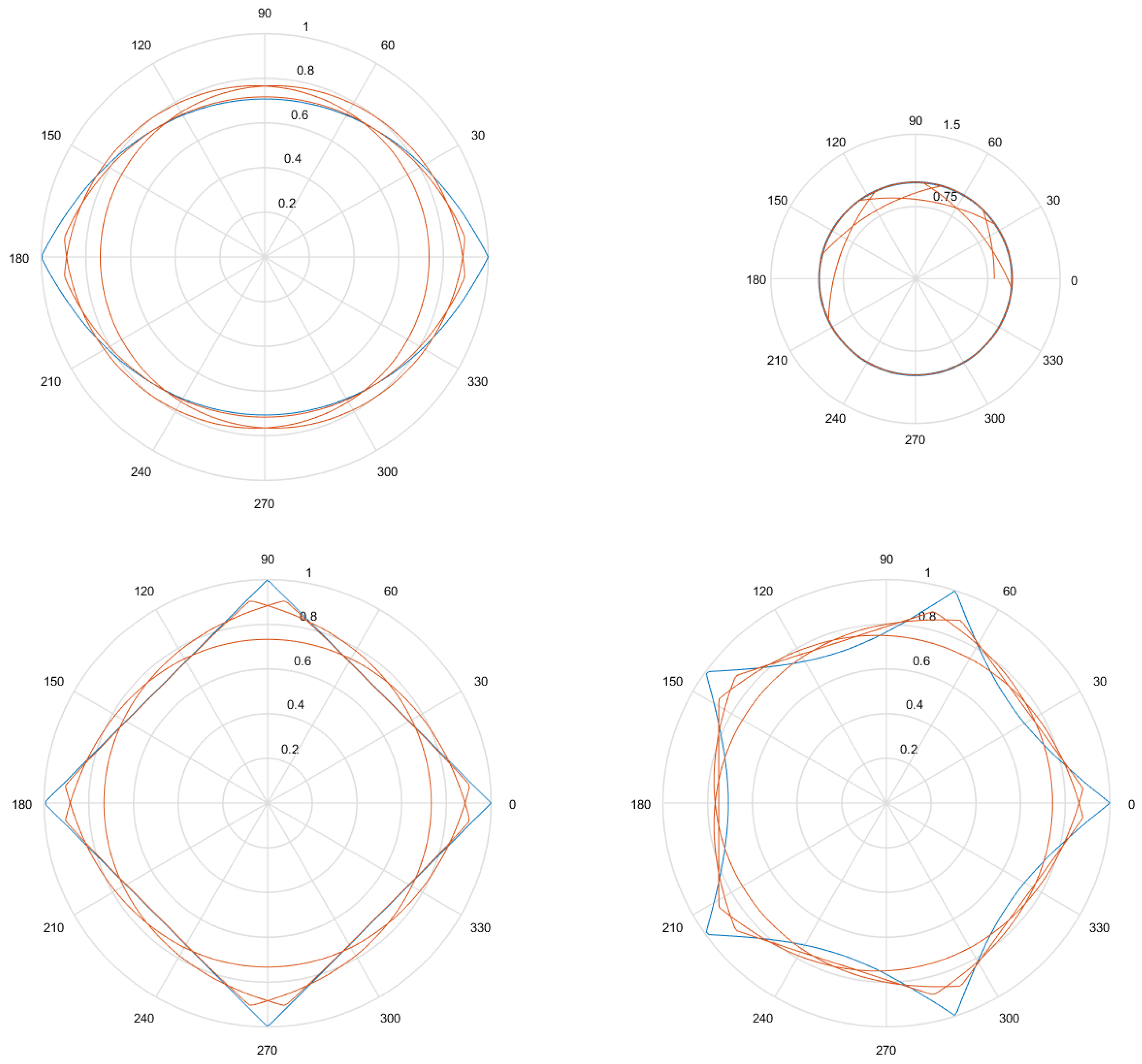
Figure 10 shows a case in which this objective function presents a better result than F 1 . The method that uses F 1 generates a Gielis curve that is self-intersecting near the polar axis, while the method that uses F 2 is not self-intersecting and because of this it presents a better adjustment to the original curve.
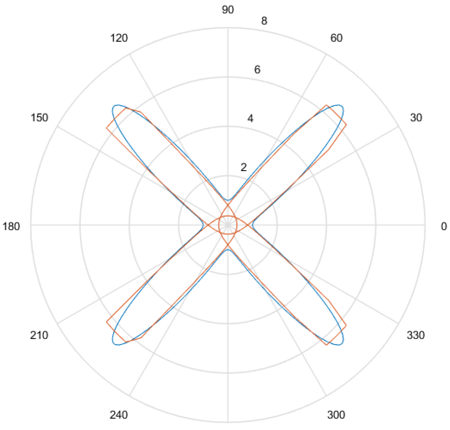
After the tests performed using Equation (13), drawbacks with this method are also observed. If length is not minimized, there are cases in which the solution spins around the original curve. Figure 11 shows examples of this drawback, the segments corresponding to the generated Gielis curves are not distant from the original curves, but spin around them.
Tests performed with this method and observed in Figure 11 show the importance of minimizing the length of the Gielis curve, aiming to avoid the repetition of segments in the obtained Gielis curves. Then, we include the length of the Gielis curve in the function given by Equation (13), and we obtain the following objective function.
F 3 ( P , F ) = f 3 ( S , P ) + f 4 ( R , P ) + f 2 ( F ) + f 3 2 ( S , P ) + f 4 2 ( R , P ) + f 2 2 ( F ) .
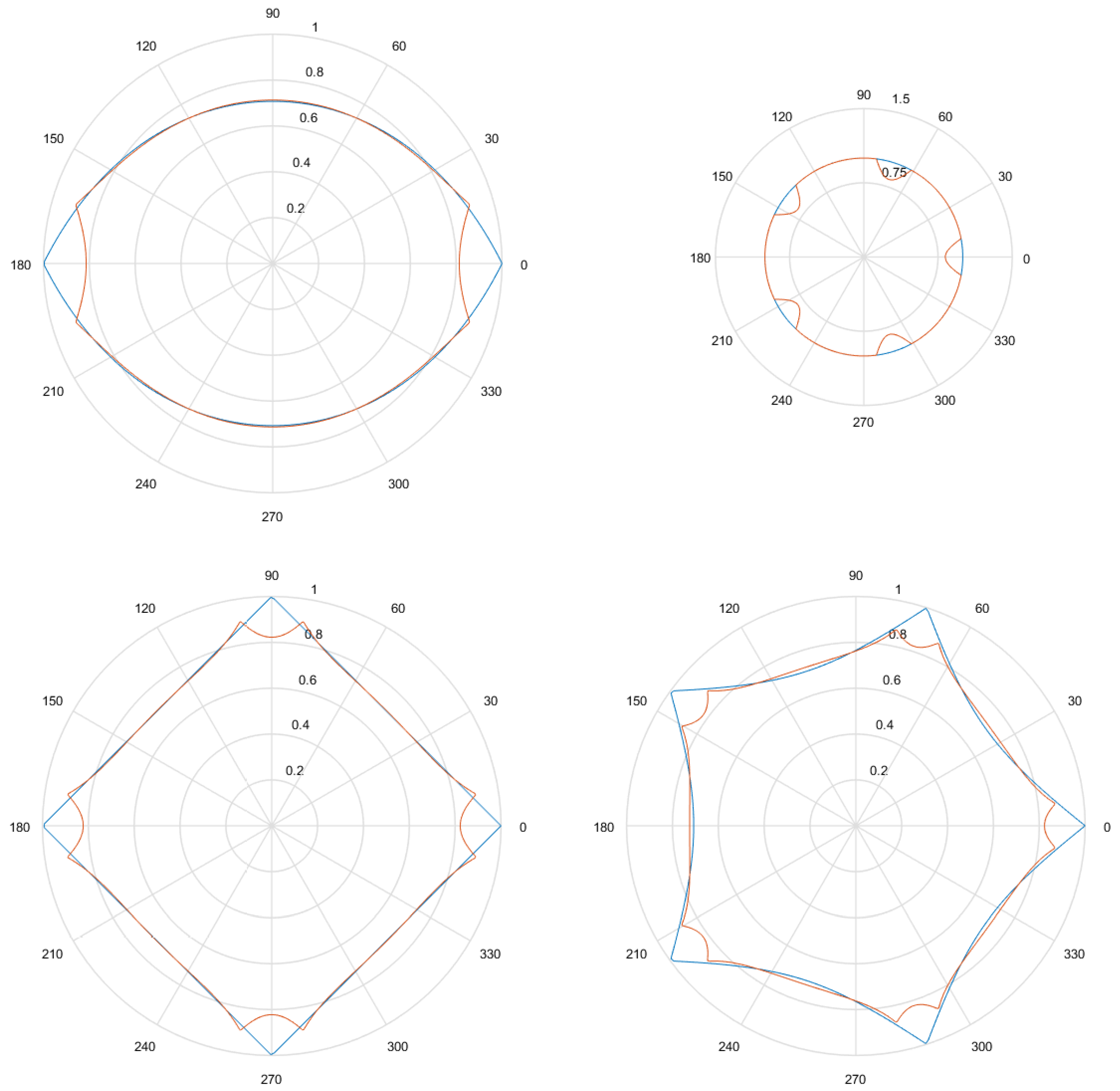
Function from Equation (14) allows to overcome the drawbacks mentioned with the previous methods and represents the main contribution of this work. Figure 12 shows the recovery of the same Gielis curves but using the objective function F 3 , thus avoiding the repetition of segments in the obtained Gielis curves. In the next section we describe the tests performed with the proposed objective functions and the results obtained.

5. Experimental Tests

In this section we present the metrics that are used to compare the aforementioned methods and the results obtained, in order to determine which method provides a better adaptation to the sample points. As input data, we used points obtained by means of a sampling from Gielis curves with known parameters, to equal intervals of θ . For each θ value, its corresponding ρ is computed, obtaining the desired amount of sample points. Next we describe the metrics used, the algorithm parameters and the results obtained.

5.1. Evaluation Metrics

Once the sample points that will be used as input data are obtained, the algorithm is executed with each method, five times per method. We take the best solution among executions, and three Gielis curves are obtained, one for each method.
Aiming to evaluate and compare the quality of the solutions, it is important an appropriate metric for evaluating the grade of similarity between two curves. This metric will be calculated between the original curve and each of the Gielis curves, allowing to compare the quality of the solutions obtained with each method. The metric is applied as follows:
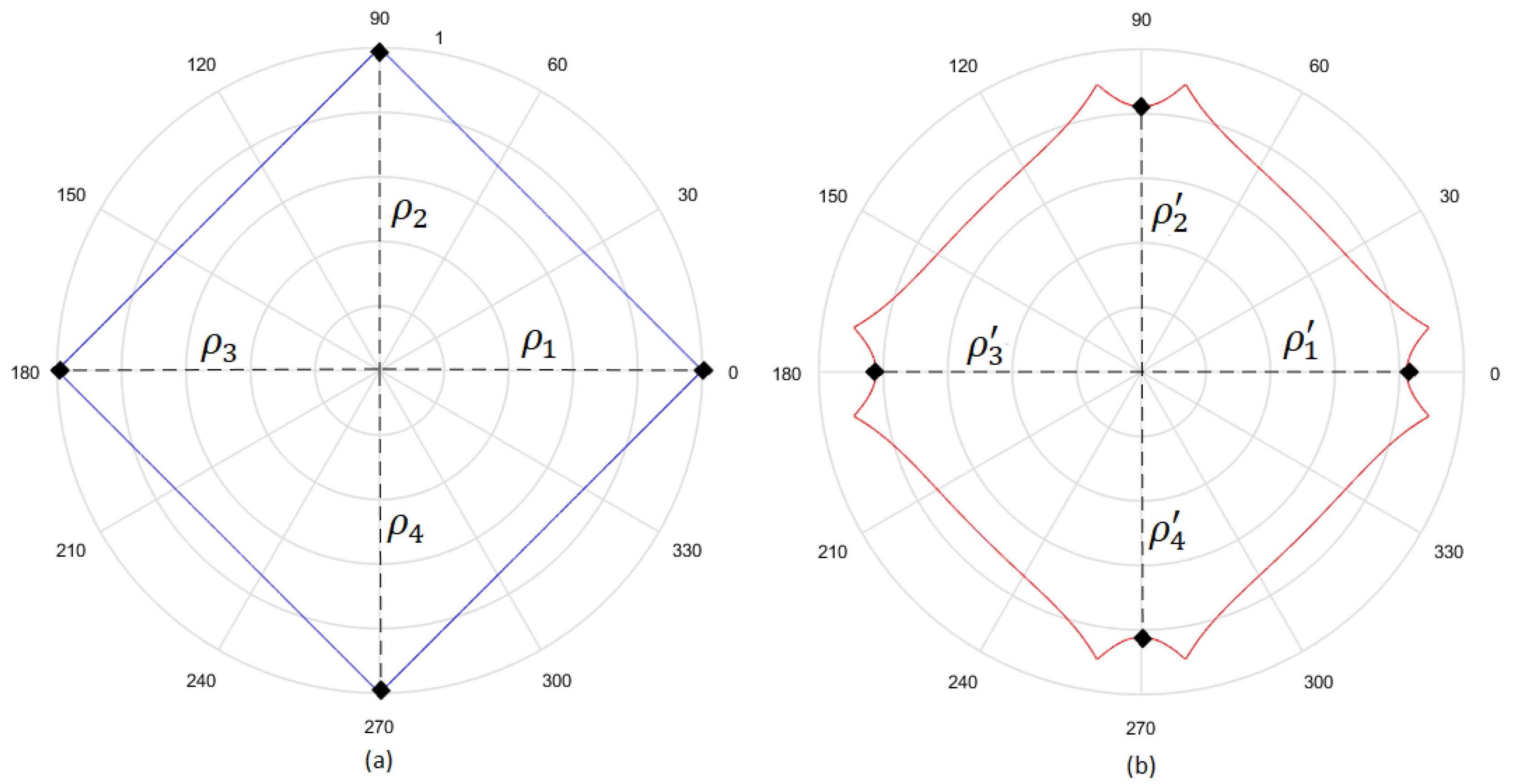
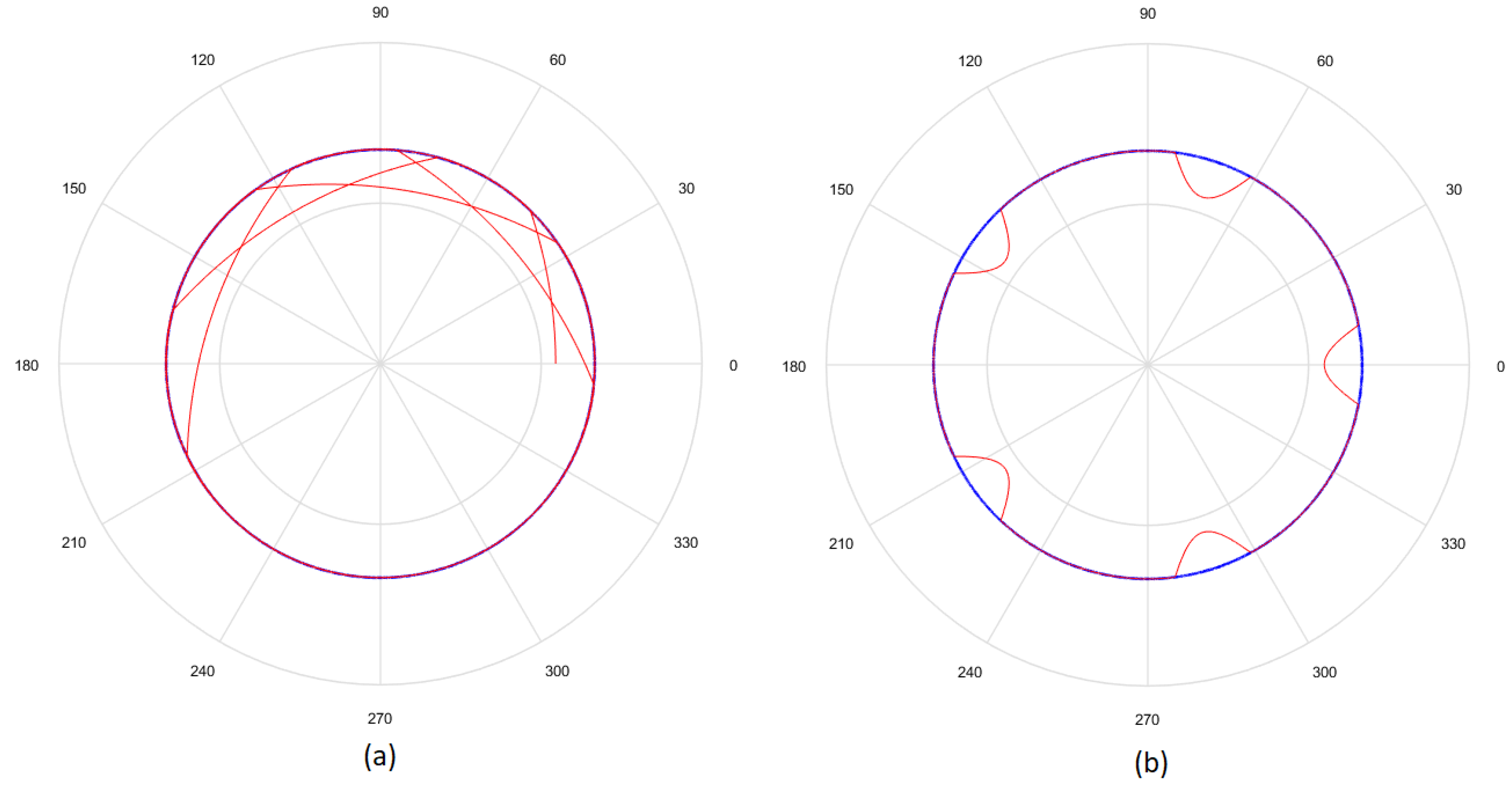
  • Considering that the tests were performed using Gielis curves with known parameters, an amount h of sample points in the original curve is obtained, to equal intervals of θ . These sample points are obtained by dividing the interval [ 0 , 2 q π ] in h equal parts. Figure 13a shows an example where h = 4 , and since q = 1 , the values of θ are π / 2 , π , 3 π / 2 , 2 π . There is in blue the original curve and in black the points obtained.
  • For each solution (one for each method), an amount h of sample points is obtained, where values of θ are the same used for the original curve. Figure 13b shows an example, corresponding to the Gielis curve obtained using objective function F 3 in Equation (14). The Gielis curve is in red and the sample points are in black.
  • Considering a h-dimensional space, finite representation of the original curve and the solutions obtained with each method are built, with polar distances ( ρ 1 , ρ 2 ,..., ρ h ) for each of them. We denote A 0 as the original curve, A 1 as the Gielis curve from the method proposed by Fougerolle et al., A 2 as the curve from the method that uses objective function F 2 from Equation (13) and A 3 for the method that uses our contribution, the objective function F 3 from Equation (14). In the example from Figure 13, there are A 0 = ρ 1 , ρ 2 , ρ 3 , ρ 4 and A 3 = ρ 1 , ρ 2 , ρ 3 , ρ 4 .
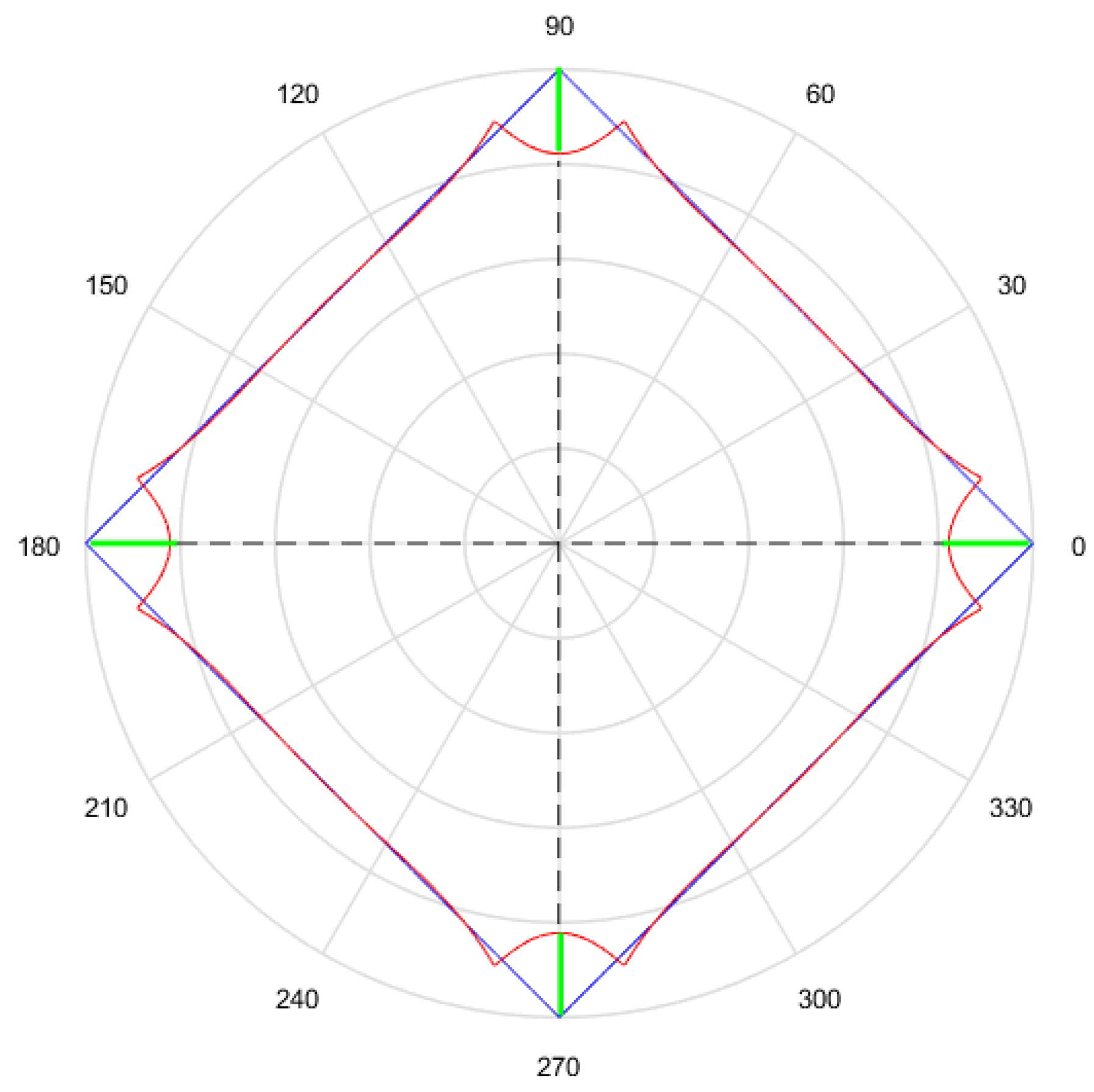
  • Finally, the Euclidean distance between A 0 and each h-dimensional point corresponding to each solution is calculated. The distance between A 0 and A 1 will be called M 1 ; between A 0 and A 2 , M 2 ; and between A 0 and A 3 , M 3 . The lower the value of the distance, the better the quality of the solution. Continuing with the example given in Figure 13, Figure 14 shows M 3 , that is equal to the root square of the sum of squares of the length of the segments in green.
The generalization of the metric for h dimensions is given by the Equation (15), denoted as
M ( A 0 , A ) = i = 1 h ( ρ i ρ i ) 2 ,
where A 0 is the set of polar distances from the original curve, A is the set of polar distances from the generated Gielis curve, h is the amount of sample points used to calculate the metric, ρ i is each of the polar distances from the generated Gielis curve and ρ i is each of the polar distances from the original curve.
Despite comparing the similarity between the original curve and the Gielis curves, this metric does not penalize the cases in which the Gielis curve spins around the original curve. This is due to the fact that the computation is performed in the interval corresponding to the original curve [ 0 , 2 q o r i g π ] , where q o r i g is the value of q corresponding to the original curve. Thus if q s o l , the parameter q of the Gielis curve, is bigger than q o r i g , segments that are in the interval [ 2 q o r i g π , 2 q s o l π ] are not penalized. Figure 15a shows in blue the original curve and in red the Gielis curve recovered using Equation (13). Figure 15b shows in blue the same original curve and in red the Gielis curve recovered using Equation (14). Visually we note that the second one is a better solution. On the contrary, according to the metric, the Gielis curve recovered using Equation (13) represents a better solution since M 2 is less than M 3 ( M 2 = 34.252844 and M 3 = 50.560416). This is due to the fact that the generated Gielis curve in Figure 15a has a value q s o l of 5 while the original curve has a value q o r i g if 1. Then, M 2 only takes 1/5 of the outline of the generated Gielis curve using Equation (13) into account. In the case of the generated Gielis curve in Figure 15b, q s o l has the same value as q o r i g , thus M 3 takes the whole solution curve into account.
For this reason, in addition to the numeric metric presented, we still perform a visual comparison to determine the quality of the solutions.

5.2. Parameters Used

Fougerolle et al. propose the following values for the evolutionary parameters [11]:
  • Mutation parameter k = 0.1.
  • Mutation probability is 0.15.
  • Minimum limit for population standard deviation σ m i n = 0.05.
  • The size of the population is 100 individuals.
  • The number of generations is 1000.
  • The intervals of the parameters of the superformula are a, b∈ [0.01, 100]; n 1 , n 2 , n 3 ∈ [0.01, 1000]; p, q∈ [1, 11].
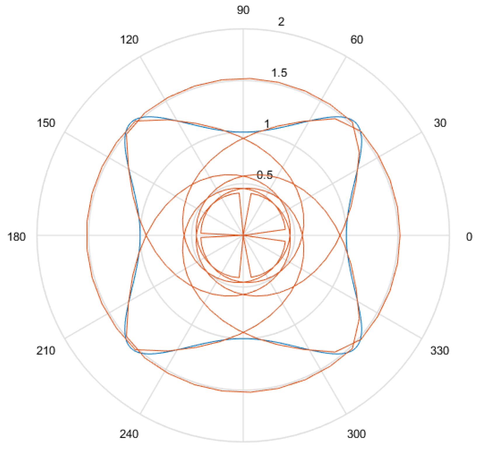
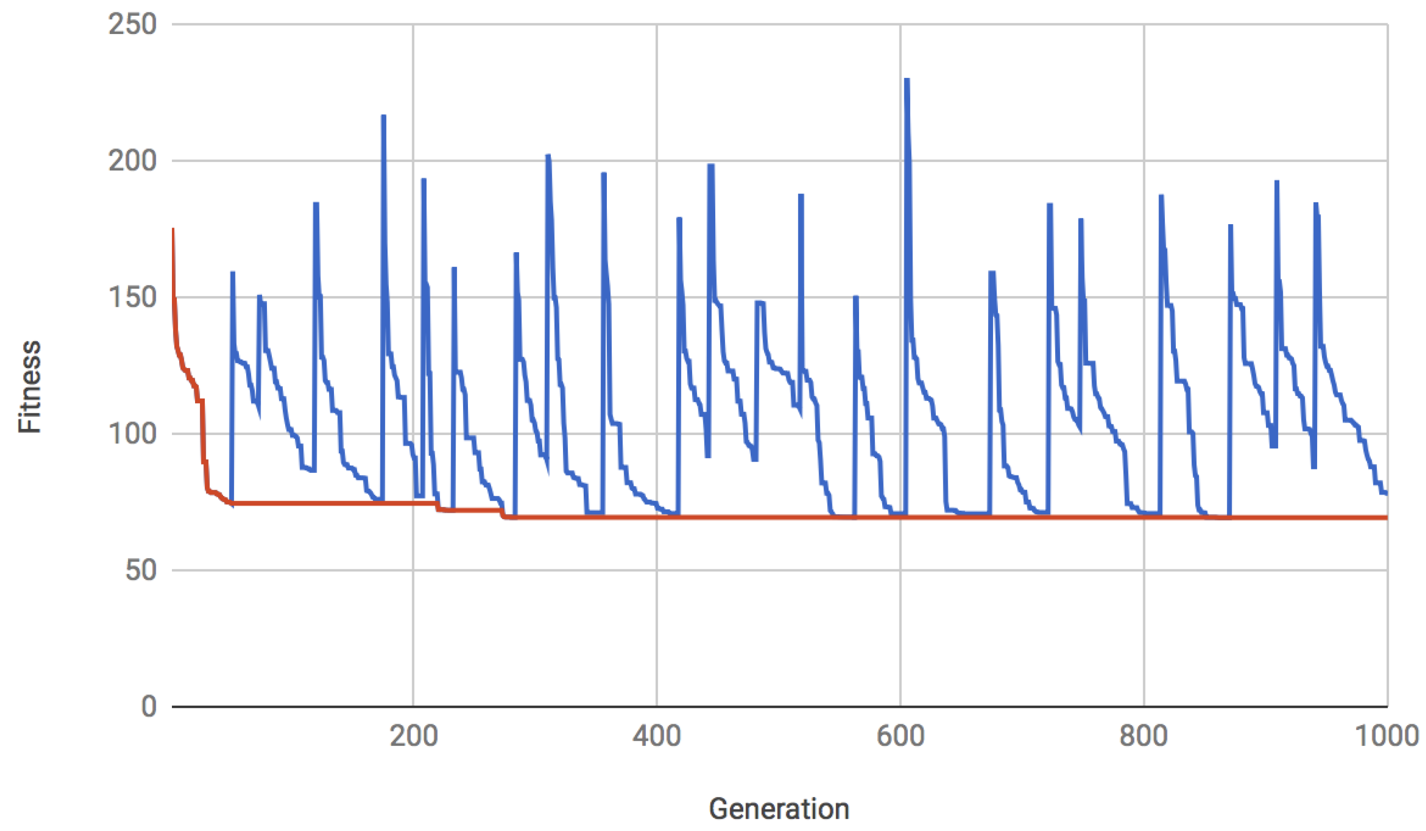
We observed the behavior of the population using F 3 with these same parameters. Figure 16 shows this behavior. The global best is in red and the bests element from each generation are in blue. We observe peaks in blue due to re-initialization of the population and we also observe in red how re-initialization favors a improvement in the fitness of the global best. After observing the behavior of the population of solutions, we decided to maintain the same parameters.
For the performed tests, the amount e of sample points is 1000. Since this work also proposes a metric for curve comparison, the amount r for computing the norms is 500,000, in order to keep the distance between the points close enough for not skipping segments from the curve.

5.3. Results

The Gielis curves in Figure 2 are considered for these experiments. Table A1 (see in Appendix A) shows these Gielis curves and the results obtained with each method. The first column shows the row number; the second shows the parameters of the original Gielis curve from which the sample points are obtained; and the third, fourth and fifth show the parameters recovered using F 1 , F 2 and F 3 , respectively. The parameters that offer the best solution according to the proposed metric are shown in bold.
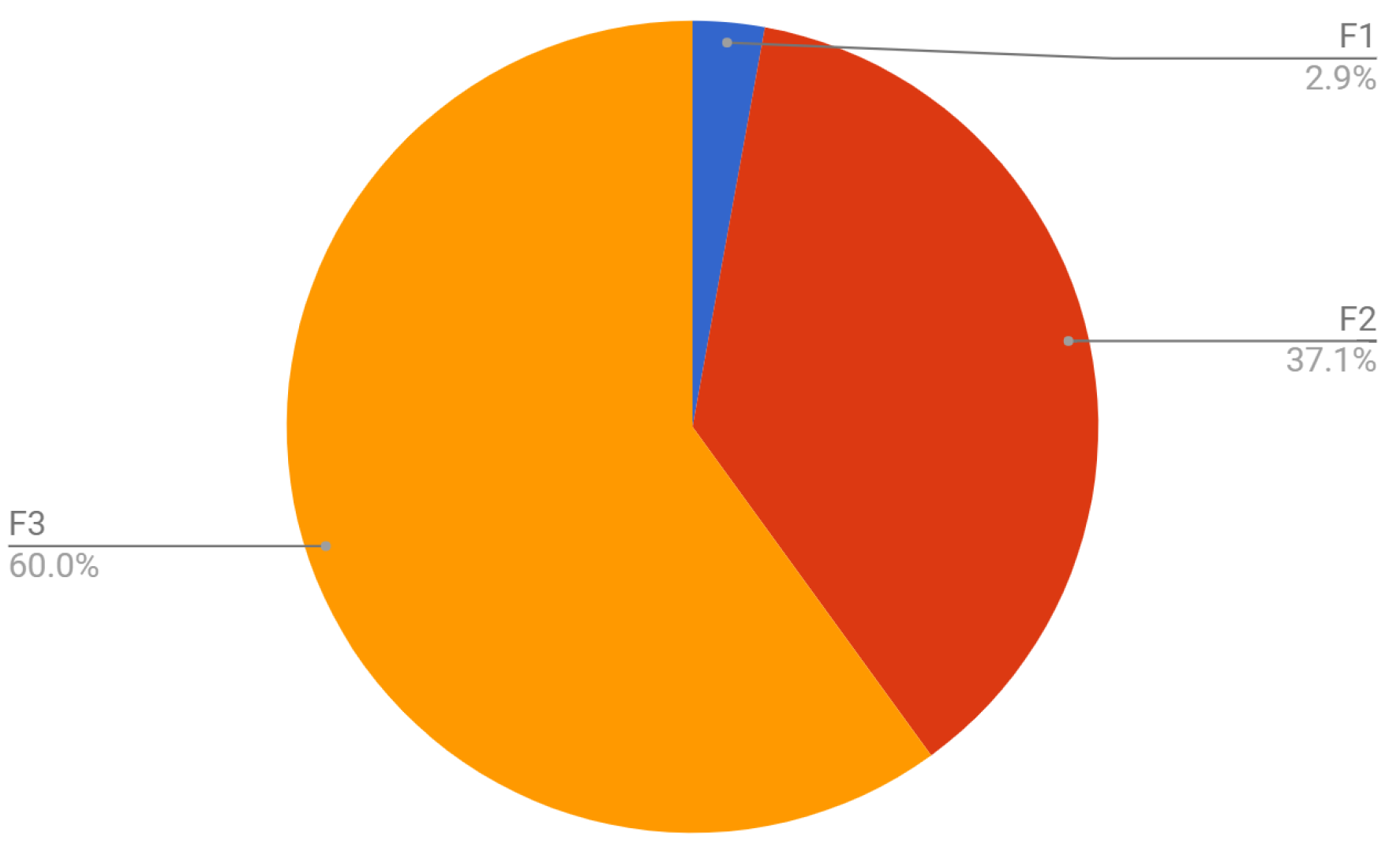
Table A2 (see in Appendix A) compares the three methods. The smaller metric values are shown in bold for each Gielis curve. The metric M 3 , corresponding to the objective F 3 , offers better solutions for the 60% of the cases, according to the applied metric. Figure 17 shows the percentages of better solutions provided by each method, according to the applied metric.
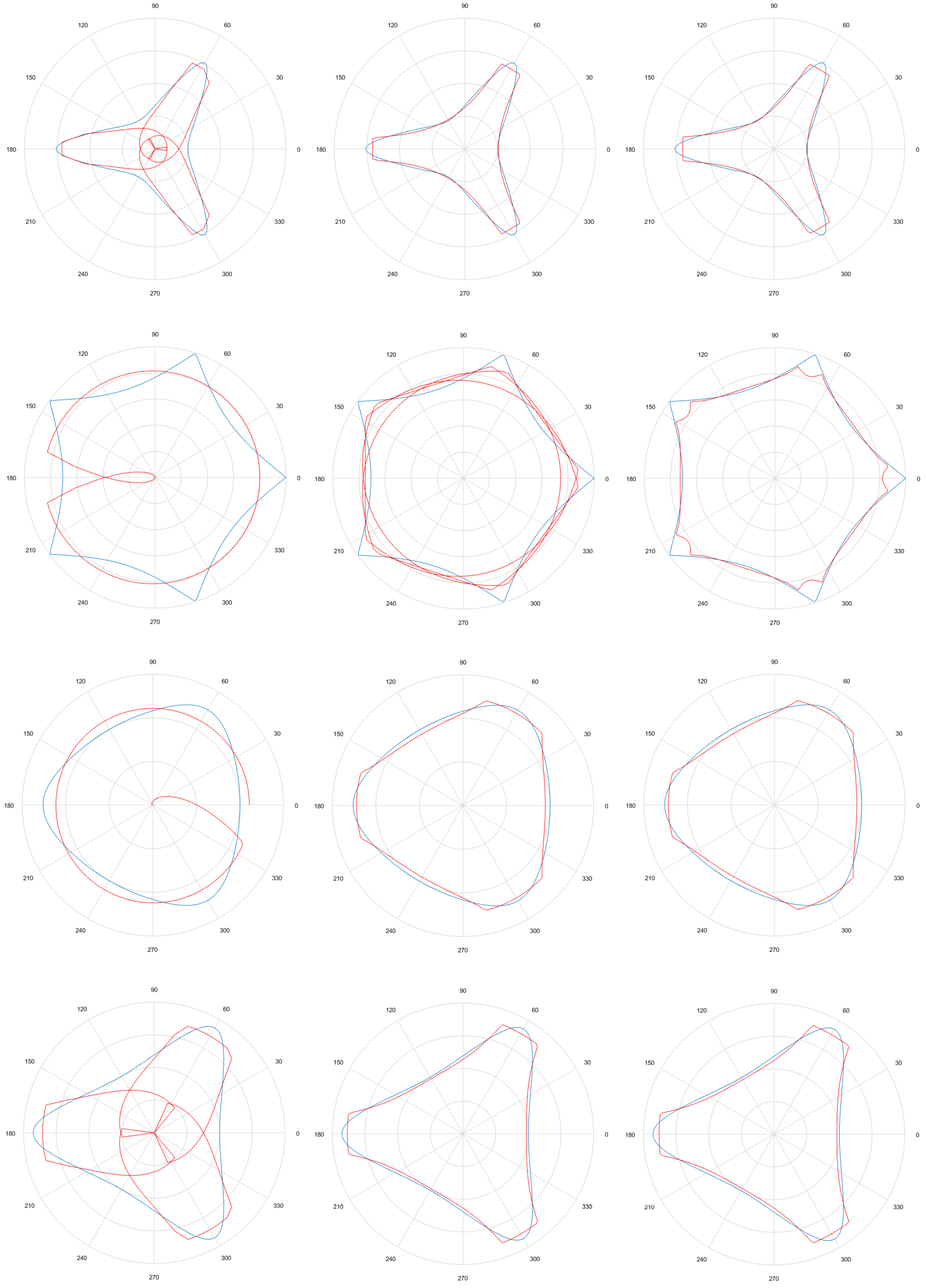
The last column of Table A2 (see in Appendix A) shows which objective function(s) provide(s) the best solution(s) according to visual comparison. We observe that in 60% of the cases, the solutions provided by F 2 and F 3 are of similar quality, better than F 1 , and in 22.9% of the cases F 3 is better than F 2 and F 1 . These cases are those in which the solutions spin around the original curves, i.e., q s o l is bigger than q o r i g . This gives a total of 82.9% of the cases in which the solution provided by F 3 is visually satisfactory. Figure 18 shows some representative examples. Each row corresponds to an original curve. The first column shows the solution obtained using the method by Fougerolle et al., the second column shows the solution obtained by F 2 , and the third column shows the solution obtained by F 3 . Rows 1, 3 and 4 show examples in which the solutions provided by F 2 and F 3 are similar; and row 2 shows an example in which the solution provided by F 2 spins around the original curve, and the solution provided by F 3 is better. It should also be noted that the solutions provided by F 3 fail to capture the corner of the shapes. This is because the length of the generated curve is included in the objective function.
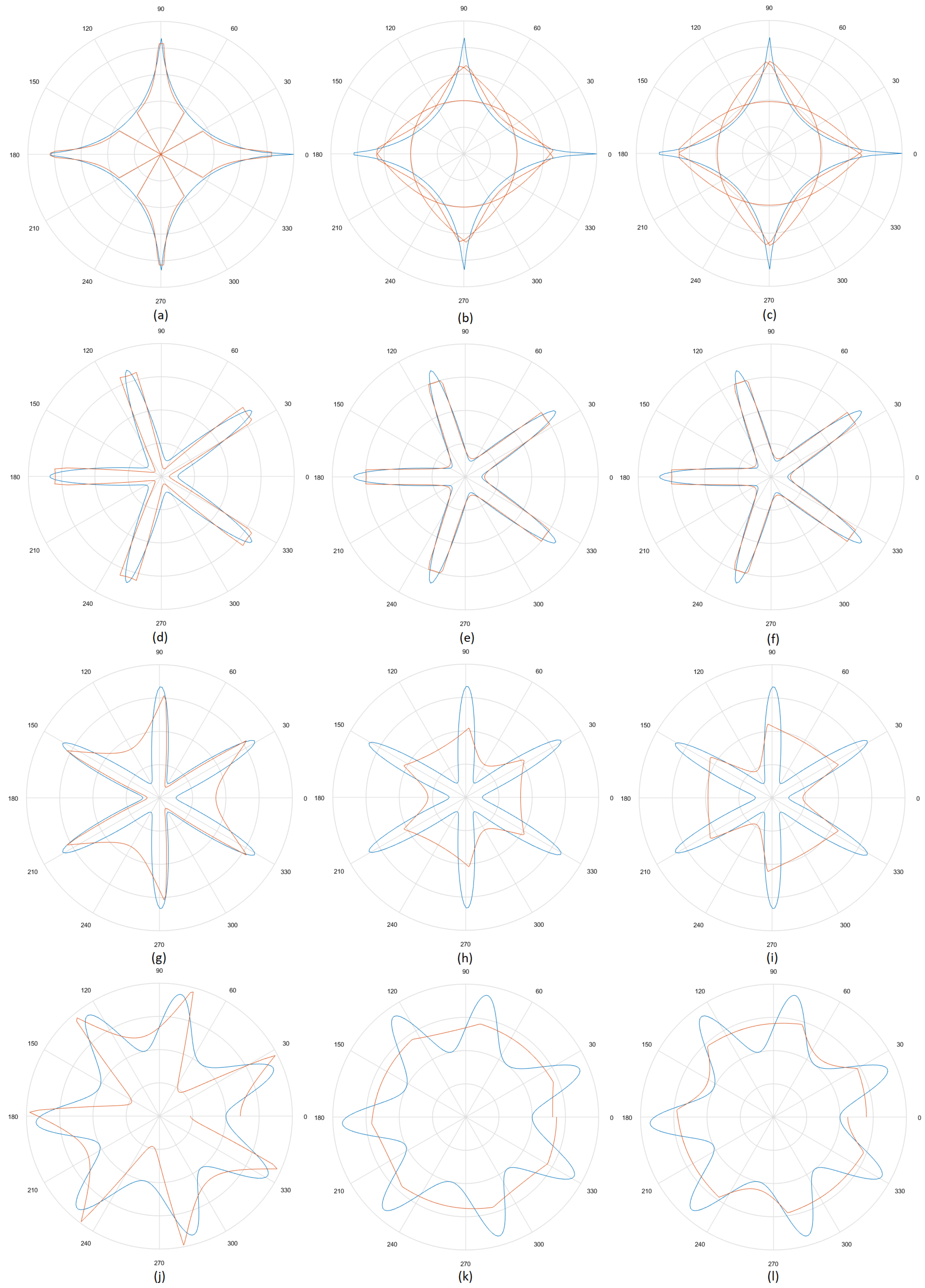
Figure 19 shows examples of exceptional cases. The first row corresponds to Gielis curve 33 from Table A2 (see in Appendix A): a case in which neither F 2 nor F 3 offer a solution of good visual quality, while F 1 provides a good general adjustment but has intersections that do not adjust to the original curve. Despite metric values, the better solution is provided by F 2 . The second row corresponds to Gielis curve 16 from Table A2 (see in Appendix A): a case in which all the methods tested provide solutions of good visual quality. According to the metric, F 3 provides the better solution. The third row corresponds to the Gielis curve 20 from Table A2 (see in Appendix A): a case in which none of the methods offers a visually satisfying solution, although F 1 is visualized as the better solution, which is confirmed by the metric. The fourth row corresponds to Gielis curve 22 from Table A2 (see in Appendix A): a case similar to the previous one, where F 1 is observed as visually better, but according to the metric F 3 offers the better solution.

6. Conclusions and Future Work

New objective functions for the recovery of Gielis curves from a set of sample points are proposed, based on a genetic algorithm proposed in the literature, which minimizes an objective function that combines Euclidean distances from the sample points to the curve, and the length of the recovered Gielis curve. The first proposed method minimizes an objective function that combines the Euclidean distances from the sample points to a curve, and from the curve to the sample points. The second proposed method minimizes another objective function, that in addition to the mentioned distances, includes the length of the recovered Gielis curve.
A visual comparison of the solutions by these methods was performed. It is observed that in 60% of the cases, the solutions provided by the proposed methods have similar quality, these being better than the ones found in the literature. In 22.9% of the cases, the second proposed method offers better solutions than the first proposed method and the literature. This totals 82.9% of cases in which the second proposed method offers better solutions than the literature.
For an objective comparison, a numeric metric for similarity between two curves has been proposed. This metric consists of obtaining sample points from both curves, building vectors with them and computing the Euclidean distance between these vectors. A lower distance implies more similarity between curves. The comparison between solutions of each method and the original curve is performed using this metric. According to the metric, we observed that the method proposed in the literature offers better solutions in only 2.9% of the cases, the first proposed method in 37.1% of the cases and the second proposed method in 60% of the cases. Although the new objective function proposed in the paper cannot faithfully represent simple curves such as squares or pentagons, it was shown to be more efficient on more complex curves compared to the method of Fougerolle et al. [11].
As future work we propose searching for other objective functions that perform well using partial data, i.e., not using all the sample points as input data: and/or with noise, i.e., with small displacements in the sample points, as done in [12]. We also propose including rotation and translation parameters to the Gielis curves respect to the origin of coordinates, in order to analyze the behavior of the objective functions with a greater amount of parameters to recover. The proposed objective function could be useful also for other metaheuristic algorithms such as simulated annealing and particle swarm. In addition, the proposed objective function can be complemented for better corner fit.

Author Contributions

Conceptualization, A.M.A. and G.G.C.; methodology A.M.A. and G.G.C.; software, A.M.A. and G.G.C.; validation, J.L.V.N.; formal analysis, G.G.C., J.L.V.N. and D.P.P.-R.; investigation, A.M.A. and G.G.C.; writing—original draft preparation, G.G.C. and J.L.V.N.; writing—review and editing, G.G.C., J.L.V.N., D.P.P.-R.. and S.A.G.; supervision J.L.V.N., S.A.G. and H.L.-A.; project administration, J.L.V.N., S.A.G. and H.L.-A.; funding acquisition, D.P.P.-R. and H.L.-A. All authors have read and agreed to the published version of the manuscript.

Funding

This research was partially funded by CONACYT (Consejo Nacional de Ciencia y Tecnología), Paraguay, by grant number 14-POS-007.

Conflicts of Interest

Authors declare no conflicts of interest.

Appendix A

Table A1. Original Gielis curves parameters and recovered values using F 1 , F 2 and F 3 . The parameters with the lowest metric are in bold.
N F1F2F3
11, 1, 2, 1, 1, 1, 10.484, 0.791, 4, 3, 98.105, 975.495, 129.0990.319, 0.832, 4, 3, 424.050, 114.101, 770.8280.914, 0.159, 4, 1, 325.238, 742.188, 59.849
21, 1, 2, 1, 1, 4, 84.588, 0.414, 4, 7, 191.792, 144.745, 383.0611.042, 93.605, 4, 1, 279.456, 290.473, 67.8241.079, 75.865, 4, 1, 498.795, 499.327, 127.463
31, 1, 2, 1, 2, 2, 20.696, 0.714, 1, 2, 6.293, 960.253, 0.1420.936, 0.704, 9, 5, 304.509, 938.779, 1.2220.893, 0.686, 10, 1, 438.576, 755.576, 0.190
41, 1, 3, 1, 1, 1, 10.297, 0.937, 6, 5, 61.612, 979.904, 316.0920.297, 0.812, 2, 1, 449.637, 118.878, 703.3620.334, 0.786, 2, 1, 607.431, 176.358, 733.708
51, 1, 3, 1, 2, 5, 70.224, 2.645, 6, 5, 906.527, 578.865, 557.2190.950, 61.136, 6, 1, 381.374, 232.292, 56.7920.978, 44.759, 6, 1, 639.679, 364.542, 103.393
61, 1, 3, 1, 2, 8, 30.228, 99.150, 6, 5, 985.876, 704.128, 83.2340.906, 91.677, 6, 1, 696.133, 434.260, 61.7870.921, 41.385, 6, 1, 145.878, 87.718, 15.638
71, 1, 3, 1, 4.5, 10, 100.193, 60.239, 6, 5, 992.387, 599.391, 129.9430.939, 63.322, 6, 1, 170.368, 77.200, 23.4200.921, 52.455, 6, 1, 261.234, 121.281, 37.254
81, 1, 3, 1, 6, 6, 65.496, 0.677, 1, 2, 62.279, 3.720, 970.2150.838, 46.878, 6, 1, 388.904, 127.007, 20.2490.837, 45.008, 6, 1, 667.043, 213.335, 34.701
91, 1, 4, 1, 1, 1, 10.394, 0.903, 1, 5, 32.366, 888.396, 93.6680.315, 0.856, 8, 3, 431.634, 116.629, 972.4330.905, 0.180, 8, 1, 395.665, 775.248, 79.420
101, 1, 4, 1, 1, 7, 80.410, 81.424, 8, 3, 164.276, 183.371, 68.6931.433, 42.658, 8, 1, 207.048, 193.665, 100.4811.367, 86.056, 8, 1, 148.692, 142.402, 60.464
111, 1, 4, 1, 4, 7, 70.191, 53.318, 8, 5, 998.697, 696.744, 92.4770.898, 52.965, 8, 1, 316.163, 129.131, 31.2480.906, 63.402, 8, 1, 362.938, 143.311, 34.214
121, 1, 4, 1, 12, 15, 151.099, 0.864, 1, 3, 34.511, 19.664, 987.3550.872, 43.314, 8, 1, 797.762, 238.308, 70.6260.889, 81.139, 8, 1, 403.617, 114.207, 30.281
131, 1, 5, 1, 1, 1, 10.848, 0.284, 2, 5, 51.066, 68.858, 585.7380.248, 0.821, 10, 3, 563.117, 119.934, 821.2610.887, 0.109, 10, 1, 236.899, 385.290, 34.413
141, 1, 5, 1, 2, 6, 60.324, 89.303, 10, 3, 963.528, 737.523, 133.6730.952, 97.590, 10, 1, 910.599, 540.286, 127.3840.934, 95.054, 10, 1, 689.156, 424.957, 95.793
151, 1, 5, 1, 2, 7, 70.330, 64.725, 10, 3, 917.122, 780.768, 174.3890.981, 70.353, 10, 1, 643.578, 427.705, 119.9790.971, 74.536, 10, 1, 560.602, 374.459, 103.183
161, 1, 5, 1, 2, 13, 130.640, 33.693, 10, 1, 319.418, 528.108, 168.2481.167, 49.765, 10, 1, 192.044, 187.902, 87.7041.162, 86.827, 10, 1, 397.561, 393.287, 159.129
171, 1, 5, 1, 4, 4, 46.275, 0.698, 1, 2, 41.642, 1.731, 932.0930.864, 51.242, 10, 1, 726.014, 316.870, 25.5470.855, 76.795, 10, 1, 397.161, 142.118, 13.019
181, 1, 6, 1, 1, 1, 10.546, 0.313, 1, 5, 59.006, 20.648, 974.6680.392, 0.755, 4, 1, 421.788, 147.881, 404.9710.442, 0.848, 4, 1, 259.665, 110.289, 515.247
191, 1, 6, 1, 1, 1, 60.698, 1.688, 1, 2, 27.366, 853.319, 2.9260.962, 2.174, 4, 1, 198.741, 953.943, 14.8750.962, 5.971, 4, 1, 227.450, 982.408, 9.511
201, 1, 6, 1, 1, 7, 82.374, 0.963, 6, 1, 81.518, 115.277, 655.8098.294, 1.447, 6, 1, 414.832, 234.199, 919.8981.202, 62.511, 6, 1, 188.828, 636.551, 61.603
211, 1, 7, 1, 1, 1, 10.228, 0.796, 1, 7, 56.159, 966.942, 51.0850.018, 0.298, 7, 1, 660.991, 48.570, 7.7660.018, 0.059, 7, 1, 466.989, 34.758, 10.356
221, 1, 7, 1, 2, 8, 41.182, 0.861, 7, 1, 195.049, 229.272, 994.4382.160, 54.319, 7, 1, 752.321, 261.122, 58.74148.455, 1.099, 7, 1, 423.512, 36.542, 497.736
231, 1, 7, 1, 10, 6, 60.489, 2.846, 1, 3, 68.889, 990.144, 3.6350.979, 44.029, 7, 1, 528.443, 177.371, 9.5060.951, 3.575, 7, 1, 420.321, 944.751, 19.205
241, 1, 2, 1, 1000, 500, 5001.608, 0.478, 1, 3, 111.856, 12.889, 893.2470.775, 82.087, 4, 1, 306.454, 58.462, 8.9420.777, 70.782, 4, 1, 366.679, 70.328, 10.946
251, 1, 4, 1, 1000, 1000, 10001.264, 0.774, 1, 3, 60.161, 24.313, 976.4590.859, 60.688, 8, 1, 656.404, 149.167, 46.3540.849, 65.430, 8, 1, 479.034, 116.408, 32.591
261, 1, 8, 1, 1, 1, 10.712, 0.554, 1, 3, 22.621, 16.037, 967.8990.018, 0.144, 8, 1, 874.896, 65.141, 6.0060.016, 0.524, 8, 1, 767.258, 54.812, 71.630
271, 1, 1, 1, 1000, 500, 5000.679, 2.652, 1, 2, 41.237, 996.966, 2.1470.794, 79.753, 2, 1, 559.873, 97.563, 16.8140.773, 17.350, 2, 1, 117.0166, 20.657, 5.439
281, 1, 5, 1, 1000, 620, 6200.682, 2.357, 1, 2, 43.564, 901.749, 3.2770.769, 26.136, 10, 1, 111.150, 25.130, 5.5580.786, 35.709, 10, 1, 262.462, 59.409, 11.482
291, 1, 8, 1, 1000, 250, 2502.634, 0.685, 1, 2, 24.175, 0.511, 979.2660.945, 8.361, 8, 1, 341.364, 853.906, 4.9770.979, 4.642, 4, 1, 135.842, 860.048, 2.014
301, 1, 1, 1, 0.5, 0.5, 0.50.340, 0.025, 2, 3, 568.301, 107.696, 241.6090.210, 0.0387, 2, 1, 551.615, 166.097, 173.4860.0516, 0.045842, 2, 1, 576.631, 91.610, 188.738
311, 1, 2, 1, 0.5, 0.5, 0.50.071, 0.042, 4, 1, 696.523, 25.619, 225.3460.269, 0.523, 4, 3, 306.789, 239.774, 332.3190.011, 0.375, 2, 1, 655.324, 137.798, 114.037
321, 1, 3, 1, 0.5, 0.5, 0.50.441, 0.033, 6, 1, 663.516, 127.949, 210.5690.014, 0.310, 3, 1, 686.319, 148.248, 105.7550.322, 0.780, 2, 1, 161.041, 139.607, 615.988
331, 1, 4, 1, 0.5, 0.5, 0.50.080, 0.027, 8, 1, 692.735, 50.256, 205.8110.271, 0.803, 8, 3, 231.396, 162.512, 997.6290.339, 0.794, 8, 3, 208.952, 182.210, 898.340
341, 1, 3, 1, 5, 18, 180.139, 47.910, 6, 7, 662.0582, 458.929, 179.9411.054, 22.793, 6, 1, 317.024, 185.602, 105.1421.024, 75.162, 6, 1, 403.783, 250.648, 96.175
351, 1, 6, 1, 20, 7, 182.072, 0.691, 1, 2, 43.927, 3.034, 999.9680.934, 25.758, 4, 1, 171.253, 336.431, 2.8830.957, 4.325, 6, 1, 328.796, 890.099, 14.078
Table A2. Gielis curves parameters and corresponding values of M1, M2 and M3. The lowest metric values are in bold. The last column shows which objective function(s) provide(s) the best solution(s) according to a visual comparison.
N FM1M2M3Visual
11, 1, 2, 1, 1, 1, 1377.05343.29334.294F3
21, 1, 2, 1, 1, 4, 81009.591218.157217.863F2, F3
31, 1, 2, 1, 2, 2, 2706.60734.25250.560F3
41, 1, 3, 1, 1, 1, 1455.75750.81651.171F2, F3
51, 1, 3, 1, 2, 5, 7686.33957.35953.733F2, F3
61, 1, 3, 1, 2, 8, 3648.76170.69168.729F2, F3
71, 1, 3, 1, 4.5, 10, 10681.30035.20138.909F2, F3
81, 1, 3, 1, 6, 6, 680.00228.24928.169F2, F3
91, 1, 4, 1, 1, 1, 1564.18951.25232.550F3
101, 1, 4, 1, 1, 7, 81749.448247.471238.497F2, F3
111, 1, 4, 1, 4, 7, 7683.15031.54629.996F2, F3
121, 1, 4, 1, 12, 15, 15114.99227.88425.087F2, F3
131, 1, 5, 1, 1, 1, 1385.33948.25233.713F3
141, 1, 5, 1, 2, 6, 6665.17043.64147.987F2, F3
151, 1, 5, 1, 2, 7, 7767.11452.24854.319F2, F3
161, 1, 5, 1, 2, 13, 13523.584176.658174.971F2, F3
171, 1, 5, 1, 4, 4, 448.11728.06925.447F2, F3
181, 1, 6, 1, 1, 1, 160.79753.94252.437F3
191, 1, 6, 1, 1, 1, 6735.62863.43463.769F2, F3
201, 1, 6, 1, 1, 7, 8966.2081112.3251170.644F1
211, 1, 7, 1, 1, 1, 1564.18952.98353.652F3
221, 1, 7, 1, 2, 8, 4227.429193.666166.163F1
231, 1, 7, 1, 10, 6, 6750.65831.69338.823F3
241, 1, 2, 1, 1000, 500, 50046.97623.66523.606F2, F3
251, 1, 4, 1, 1000, 1000, 100084.70924.65626.681F2, F3
261, 1, 8, 1, 1, 1, 163.03353.16453.052F2
271, 1, 1, 1, 1000, 500, 500735.50620.49722.454F2, F3
281, 1, 5, 1, 1000, 620, 620739.20329.09327.489F2, F3
291, 1, 8, 1, 1000, 50, 25071.04335.78829.789F2, F3
301, 1, 1, 1, 0.5, 0.5, 0.5235.73328.12729.374F2
311, 1, 2, 1, 0.5, 0.5, 0.5102.92782.17873.118F1
321, 1, 3, 1, 0.5, 0.5, 0.5106.66676.11969.748F1
331, 1, 4, 1, 0.5, 0.5, 0.5148.70772.19175.124F2, F3
341, 1, 3, 1, 5, 18, 181103.13862.80763.799F2, F3
351, 1, 6, 1, 20, 7, 1848.78754.22742.373F3

References

  1. Forestiere, C.; He, Y.; Wang, R.; Kirby, R.M.; Negro, L.D. Inverse Design of Metal Nanoparticles’ Morphology. ACS Photonics 2016, 3, 68–78. [Google Scholar] [CrossRef] [Green Version]
  2. Tzarouchis, D.; Ylä-Oijala, P.; Ala-Nissilä, T.; Sihvola, A. Plasmonic properties and energy flow in rounded hexahedral and octahedral nanoparticles. J. Opt. Soc. Am. 2016, 33, 2626–2633. [Google Scholar] [CrossRef] [Green Version]
  3. Leonardis, A.; Jaklic, A.; Solina, F. Superquadrics for segmenting and modeling range data. IEEE Trans. Pattern Anal. Mach. Intell. 1997, 19, 1289–1295. [Google Scholar] [CrossRef] [Green Version]
  4. Gielis, J. A generic geometric transformation that unifies a wide range of natural and abstract shapes. Am. J. Bot. 2003, 90, 333–338. [Google Scholar] [CrossRef] [PubMed]
  5. Vega, V.; Sidibé, D.; Fougerolle, Y. Road signs detection and reconstruction using gielis curves. In Proceedings of the International Conference on Computer Vision Theory and Applications, Rome, Italy, 24–26 February 2012; pp. 393–396. [Google Scholar]
  6. Tassadit, A.; Macías, D.; Sanchez-Gil, J.A.; Adam, P.-M.; Rodríguez-Oliveros, R. Metal nanostars: Stochastic optimization of resonant scattering properties. Superlattices Microstruct. 2011, 49, 288–293. [Google Scholar] [CrossRef] [Green Version]
  7. Macías, D.; Adam, P.-M.; Ruíz-Cortes, V.; Rodríguez-Oliveros, R.; Sanchez-Gil, J.A. Heuristic optimization for the design of plasmonic nanowires with specific resonant and scattering properties. Opt. Express 2012, 20, 13146–13163. [Google Scholar] [CrossRef] [PubMed]
  8. Duda, R.O.; Hart, P.E. Pattern Classification and Scene Analysis; Wiley: New York, NY, USA, 1973. [Google Scholar]
  9. Fougerolle, Y.D.; Gribok, A.; Foufou, S.; Truchetet, F.; Abidi, M.A. Boolean operations with implicit and para- metric representation of primitives using R-functions. IEEE Trans. Vis. Comput. Graph. 2005, 11, 529–539. [Google Scholar] [CrossRef] [PubMed]
  10. Barr, A.H. Superquadrics and angle-preserving transformations. IEEE Comput. Graph. Appl. 1981, 1, 11–23. [Google Scholar] [CrossRef] [Green Version]
  11. Fougerolle, Y.D.; Gielis, J.; Truchetet, F. A robust evolutionary algorithm for the recovery of rational Gielis curves. Pattern Recognit. 2013, 46, 2078–2091. [Google Scholar] [CrossRef]
  12. Gielis, J.; Caratelli, D.; Fougerolle, Y.; Ricci, P.E.; Tavkelidze, I.; Gerats, T. Universal Natural Shapes: From Unifying Shape Description to Simple Methods for Shape Analysis and Boundary Value Problems. PLoS ONE 2012, 7, e29324. [Google Scholar] [CrossRef]
  13. Mishra, S.K. Some Experiments on Fitting of Gielis Curves by Simulated Annealing and Particle Swarm Methods of Global Optimization. IUP J. Comput. Math. 2011, 4, 50–59. Available online: https://ssrn.com/abstract=2141745 (accessed on 3 June 2020). [CrossRef] [Green Version]
  14. Von Seggern, D.H. Practical Handbook of Curve Design and Generation; CRC Press: Boca Raton, FL, USA, 1994. [Google Scholar]
  15. Yang, X.S. Nature-Inspired Metaheuristic Algorithms; Luniver Press: Frome, UK, 2010. [Google Scholar]
  16. Blum, C.; Roli, A. Metaheuristics in combinatorial optimization: Overview and conceptual comparison. ACM Comput. Surv. (CSUR) 2003, 35, 268–308. [Google Scholar] [CrossRef]
  17. Falkenauer, E. Genetic Algorithms and Grouping Problems; John Wiley & Sons, Inc.: Hoboken, NJ, USA, 1998. [Google Scholar]
  18. Jäntschi, L.; Bălan, M.C.; Sestraş, R.E. Results of evolution supervised by genetic algorithms. arXiv 2010, arXiv:1009.091. [Google Scholar] [CrossRef] [Green Version]
  19. Janežič, D.; Jäntschi, L.; Bolboacă, S.D. Sugars and sweeteners: Structure, properties and in silico modeling. Curr. Med. Chem. 2020, 27, 5–22. [Google Scholar] [CrossRef]
  20. Bokhabrine, Y.; Fougerolle, Y.; Foufou, S.; Truchetet, F. Genetic algorithms for Gielis surface recovery from 3D data sets. In Proceedings of the 2007 IEEE International Conference on Image Processing, San Antonio, TX, USA, 16 September–19 October 2007; IEEE: Piscataway, NJ, USA, 2007. [Google Scholar]
  21. Wang, X.; Wang, H. Classification by evolutionary ensembles. Pattern Recognit. 2006, 39, 595–607. [Google Scholar] [CrossRef]
  22. Maulik, U.; Bandyopadhyay, S. Genetic algorithm-based clustering technique. Pattern Recognit. 2000, 33, 1455–1465. [Google Scholar] [CrossRef]
  23. Cross, A.D.; Myers, R.; Hancock, E.R. Convergence of a hill-climbing genetic algorithm for graph matching. Pattern Recognit. 2000, 33, 1863–1880. [Google Scholar] [CrossRef] [Green Version]
  24. Rvachev, V.L. Theory of R-Functions and Some Applications; Naukova Dumka: Kiev, Ukraine, 1982. [Google Scholar]
  25. Shapiro, V. Theory of R-Functions and Applications: A Primer; Cornell University: Ithaca, NY, USA, 1991. [Google Scholar]
  26. Shapiro, V. Semi-analytic geometry with R-functions. ACTA Numer. 2007, 16, 239–303. [Google Scholar] [CrossRef] [Green Version]
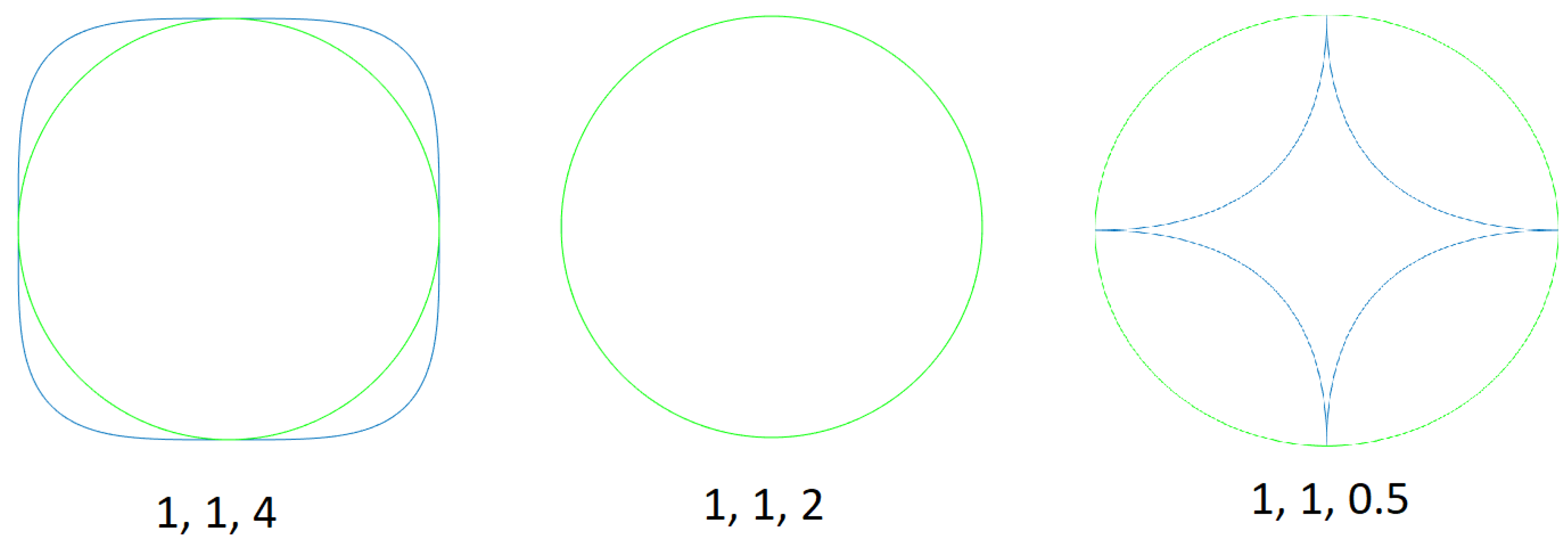
Figure 1. Superellipse examples in blue. In green, circles (given by Equation (1) using n = 2 , a = b = 1 ). The first curve is circumscribed by the circle, the second curve is a circle and the third curve is inscribed in the circle. Values of a, b and n from Equation (1) are shown, respectively.
Symmetry 12 01016 g001
Figure 2. Gielis curves examples. For all the examples, a = b = 1, the values that are shown correspond to m, n 1 , n 2 and n 3 from Equation (2), respectively.
Symmetry 12 01016 g002
Figure 3. Crossover examples. For each gene, a random value α between 0 and 1 is obtained. If α 0.5 the first child takes the gene from the first father (in blue) and the second child takes the gene from the second father (in green). If α > 0.5 the first child takes the gene from the second father (in green) and the second child takes the gene from the first father (in blue). (a) Shows crossover in which the condition that p and q should be relative primes is not fulfilled. (b) Shows the correction applied in order to fulfill the condition.
Symmetry 12 01016 g003
Figure 4. Variation of parameter p. The curves generated by Equation (2) are shown in blue. a , b , p , q , n 1 , n 2 , n 3 from Equation (2) are shown between braces.
Symmetry 12 01016 g004
Figure 5. Shortest Euclidean Distance (SED) example. The SED is calculated for the curve in blue. The sample points are in green, and the segment that indicates the shortest distance from the point to the curve is in black.
Symmetry 12 01016 g005
Figure 6. Example of the recovery of Gielis curves minimizing function in Equation (6). In blue is the original curve and in red is the recovered curve.
Symmetry 12 01016 g006
Figure 7. Recovery of Gielis curve minimizing function in Equation (9). The original curve is in blue and the recovered curve is in red.
Symmetry 12 01016 g007
Figure 8. The SED from P j to the curve (in red) is shown in green. d( P j , S j ) is shown in yellow. The sample points are in blue and the generated curve is in red.
Symmetry 12 01016 g008
Figure 9. Distance d 2 given by Equation (11) is shown in green. The sample points are in blue and the points corresponding to the generated curve are in red.
Symmetry 12 01016 g009
Figure 10. In blue are the original curves and in red are the solution curves. At the left is the result of minimizing function F 1 given by Equation (9) and at the right is the result of minimizing function F 2 given by Equation (13).
Symmetry 12 01016 g010
Figure 11. Examples of conflicting cases using F 2 , given by Equation (13). In blue are the original curves and in orange are the solution curves.
Symmetry 12 01016 g011
Figure 12. Same curves as Figure 11 but recovered using F 3 given by Equation (14). In blue are the original curves and in orange are the solution curves.
Symmetry 12 01016 g012
Figure 13. Sample points for the computation of the comparison metric given by Equation (15). (a) In blue is the original curve and (b) in red is the Gielis curve. In black are the points obtained.
Symmetry 12 01016 g013
Figure 14. M 3 . The original curve is in blue and the Gielis curve is in red. The metric corresponds to the root square of the sum of squares of the segments in green, i.e., Euclidean distance.
Symmetry 12 01016 g014
Figure 15. Example of a drawback with the proposed metric M 3 . (a,b) The original curve is in blue and the Gielis curve is in red.
Symmetry 12 01016 g015
Figure 16. Example of the behavior of the population using F 3 . The global best is in red and the best elements from each generation are in blue.
Symmetry 12 01016 g016
Figure 17. Better solutions according to the proposed metric M 3 .
Symmetry 12 01016 g017
Figure 18. Representative examples of the solutions obtained using each method. The original curves are in blue and the Gielis curves are in red. First column corresponds to the method proposed by Fougerolle et al. Second column corresponds to F 2 (Equation (13)), and the third column corresponds to F 3 (Equation (14)).
Symmetry 12 01016 g018
Figure 19. The original curves are in blue and the Gielis curves are in red. First column (a,d,g,j) corresponds to the method proposed by Fougerolle et al. Second column (b,e,h,k) corresponds to F 2 (Equation (13)), and the third column (c,f,i,l) corresponds to F 3 (Equation (14)).
Symmetry 12 01016 g019
Table 1. Example of an R-function with its corresponding signs.
xy f ( x , y )
+++
++
++