A Machine-Learning-Based Approach to Predict the Health Impacts of Commuting in Large Cities: Case Study of London

Abstract

The daily commute represents a source of chronic stress that is positively correlated with physiological consequences, including increased blood pressure, heart rate, fatigue, and other negative mental and physical health effects. The purpose of this research is to investigate and predict the physiological effects of commuting in Greater London on the human body based on machine-learning approaches. For each participant, the data were collected for five consecutive working days, before and after the commute, using non-invasive wearable biosensor technology. Multimodal behaviour, analysis and synthesis are the subjects of major efforts in computing field to realise the successful human–human and human–agent interactions, especially for developing future intuitive technologies. Current analysis approaches still focus on individuals, while we are considering methodologies addressing groups as a whole. This research paper employs a pool of machine-learning approaches to predict and analyse the effect of commuting objectively. Comprehensive experimentation has been carried out to choose the best algorithmic structure that suit the problem in question. The results from this study suggest that whether the commuting period was short or long, all objective bio-signals (heat rate and blood pressure) were higher post-commute than pre-commute. In addition, the results match both the subjective evaluation obtained from the Positive and Negative Affect Schedule and the proposed objective evaluation of this study in relation to the correlation between the effect of commuting on bio-signals. Our findings provide further support for shorter commutes and using the healthier or active modes of transportation.

1. Introduction

Stress refers to physical, mental, or emotional reactions in response to changes that occur in the body. It is among the physiological symptoms that are frequently seen in people who work [1]. It is one of the major problems in modern society. It is the body’s reaction to feeling threatened or under pressure. However, too much stress can affect our mood, our body and our relationships—especially when it feels out of control. It can make us feel anxious and irritable and affect our self-esteem. There are many possible causes of stress, for example, the pressure at work, school or home, illness, or difficult or sudden life events and many other things. Stress is responsible for abnormal responses in the autonomic nervous system (ANS), which is combined with the sympathetic nervous system (SNS) and the parasympathetic nervous system (PNS) under antagonistic control.

For millennia, we have understood that heart rate (HR) responds to stress. When we are overwhelmed with stress, in our body, adrenal glands are triggered to release the hormones cortisol and adrenaline. These can make our heart beat faster and raise our blood pressure. Many parameters can indicate stress levels in the body in medical contexts; these include heart rate variability (HRV), galvanic skin response, cortisol, blood pressure (BP), electroencephalogram (EEG), and respiratory activity [1]. In this context, the heart rate variability (HRV), i.e., the variation in the time interval between heartbeats, is known to be a reliable non-invasive biomarker of the ANS. Using BP, heart rate, and HRV, it is possible to monitor the activity of the sympathetic and parasympathetic nervous systems [2]. Apart from such physically observable phenomena or responses of the body, various technologies have also been developed to detect stress levels using physiological signals; for example, in a study conducted by Akane, they used wearable sensor and mobile phones to detect the stress. There are many novel wearable devices such as Olive, Spire, BreathAcoustics, and Gizmodo integrated with various biosensors that help people monitor stress and organise their daily life accordingly. In a study conducted by Vrijkotte, work stress was evaluated using BP, heart rate, and HRV [3]. The study resulted that the high imbalance (a combination of high effort and low reward at work) was statistically correlated with a higher heart rate during work and higher systolic blood pressure during work and leisure time. Some of the studies are based on stress questionnaires, which are commonly used by psychologists to detect patients’ stress levels; for example, a research conducted by Sheldon Cohen used a questionnaire for the reliability and validity of a 14-item instrument, the Perceived Stress Scale (PSS), which is designed to measure the degree to which situations in one’s life are appraised as stressful [1]. Heart rate is also used as a parameter in various studies on stress identification [4].

Thus, we herein report the application of artificial intelligence to predict the effect of commute on BP and heart rate. We include as participants individuals who commute to and from work regularly. The participants are stratified based on how they commute to work (public transport, driving, or cycling/walking). Our approach will allow us to measure the effects during and after the period of commuting for a group of people. For this purpose, cutting-edge technology is used in this research: the MySignals device. We applied machine-learning approaches to predict the effect of a long commute on human heart rate and BP in the London area. Machine learning provides systems with the ability to learn and improve automatically from experience without being programmed explicitly. The value of machine learning in healthcare is its ability to process huge datasets beyond the scope of human capability and then reliably convert an analysis of that data ultimately leading to better outcomes. Machine learning provides systems with the ability to learn and improve automatically from the experience; it enables a broader range of scenarios (different commuting types, different environment, etc.) to be explored outside of the data. Moreover, it will help us provide a generalised module with the ability to help the employers provide the right support for their employees who have a long commute. In this process, we have chosen from among the various widely accepted artificial intelligence techniques those which are most relevant to our research.

2. Literature Review and the State of the Art

The Sano–Picard framework [1] applied correlation analysis to find statistically significant features associated with stress and used machine learning to classify whether the participants were stressed or not. They collected five-day physiological and behavioural data, including skin conductance. They obtained over 75% accuracy for low and high perceived stress recognition using a combination of mobile phone usage and sensor data. In a study conducted by Vrijkotte, BP, heart rate, and HRV were used to evaluate work stress [3]. The results of that study suggest that work stress can cause increased heart-rate reactivity to a stressful workday, an increase in systolic BP, and lower vagal tone. In another study, Hudson [4] used a machine-learning approach to predict increases in BP.

As today’s world is moving towards intelligent systems, the demand for collaboration between various fields is increasing. Artificial intelligence techniques have been widely used in various forms of medical treatment. In this study, we are leveraging collaboration between AI and medical data analysis. By using artificial intelligence, this study aims to investigate how different psychophysical signals of healthy participants are collected to define a solid starting point for studying the impact of commuting on BP and heart rate.

Similarly, in a report produced by the Royal Society for Public Health (RSPH), the main findings were the health status, level of happiness, and satisfaction were lower for people who had longer commutes [5]. In that report, factors such as how long the commute takes and the type of commute (e.g., by public transport, cycling, or driving) have an impact on how individuals feel about the commute. Commuting is one of the biggest lifestyle challenges in Greater London, as Londoners spend an average of 56 min travelling, rising to 79 min. For example, active commuting, which involves walking, cycling or using public transport, is associated with lower levels of stress, and long commutes tend to be associated with more stress. The number of people who spend more than two hours commuting to and from work every day has jumped by 72% over the past decade to more than three million, according to the Trade Union Congress (TUC), as published by The Guardian. However, most of the studies on the effects of stress on commuting have been based on self-report questionnaires.

Machine learning is a new field that is focused on the development of systems that can automatically learn from data and create highly accurate predictive models. It has attracted considerable research interest towards developing smart digital health interventions. These interventions have the potential to revolutionise health care and lead to substantial outcomes for patients and medical professionals [6]. It has already been implemented in many health-related studies such as obesity prediction. In that study, they created a framework that combines both the statistical and extraction-based methods with appropriate feature representation/selection strategy [7]. In addition, software architecture was designed for the classification of information from patient electronic records; the architecture was formed by a classification layer that includes a linguistic module and machine learning classification modules [8]. Artificial neural network (ANN) classification techniques are used to detect the region of tumours in the clinical datasets of patients with laryngeal tumours [9].

Artificial intelligence has been trending in the field of medicine and health care. An overview of recent studies indicate that much artificial intelligence, machine learning, and deep learning techniques are being applied for various purposes, including the detection, prediction, diagnosis, and treatment of diseases, thereby reducing instances of human error in medical data analysis and processing. Variously, ANN techniques, regression and classification techniques, deep-learning convolutional neural networks, fuzzy logic, rule-based expert system techniques, and machine-learning techniques have been found to obtain better respective results when applied to detection systems, data analysis, data visualisation and classification methods. Feed-forward neural networks are the most popular static network. One study found that the feed-forward ANN technique has much better optimisation and precision when compared with the statistical multiple regression analysis techniques [8]. In this paper, different algorithms, such as quasi-Newton, gradient descent, and genetic algorithms, were used to train the ANN. In another study, it was noted that an ANN technique performed better than multiple regression techniques [10]. An ANN technique with a back-propagation algorithm was compared with statistical and machine-learning multiple-regression techniques to conduct a continuous estimation of blood pressure. Artificial intelligence technologies can provide better accuracy and save a significant amount of time on classification and quantification in positron emission tomography [11]. ANN techniques were found to be highly reliable and more effective in a recent study on machine learning and stress assessment [12]. Using risk factors such as stress, diabetes, obesity, smoking, salt intake, BP, and cholesterol as inputs, diagnosis of hypertension is easily predicted by applying ANN techniques. A decision tree algorithm was used for continuous BP measurement to predict BP at a continuous rate based on human physiological data from ECG signals and heart-rate reading [13]. Finally, a support vector machine-based hardware platform was used for blood-pressure prediction. ANNs are one of the best artificial intelligence (AI) technologies with the capacity to classify, measure the region of interest precisely, and model the clinical evaluation [14]. In this study, the support vector machine, recurrent neural networks, and the K-nearest neighbour algorithm are used to confirm whether heart rate and BP would be higher post-commute compared to pre-commute. Feed-forward neural networks, linear discriminant analysis (LDA), and decision tree techniques are used to confirm whether the systolic BP is higher in longer commutes versus shorter. Before applying these machine-learning techniques, a feature selection phase was conducted using several correlation methods.

Feed-forward neural networks are one of the most effective ANN techniques. In this technique, the information only moves in the forward direction. There are three main layers in this network: the input layer, the hidden layer, and the output layer. In a study, the classification of heart diseases using HRV signals was performed for normal patients and patients with congestive heart failure (CHF) and myocardial infarction. The data were taken from ECG recordings, and a multi-layer feed-forward neural network was used for their classification [15]. Three different methods (time-domain, frequency-domain, and non-linear methods) were used to select the inputs to the neural network classifier. The results obtained based on the non-linear methods were used as a high accuracy rate for classifying heart diseases was achieved. A multi-layer feed-forward neural network consisting of an input layer, multiple hidden layers, and an output layer was used to predict the probability of occurrence of hypertension [16]. This technique was also used in feature selection in ischemic heart disease identification [17]. LDA is now a widely used technique in the field of artificial intelligence and machine learning and its associated methods, including statistical analysis, data analysis, pattern recognition, and classifier models. It can predict the value of the dependent variable using the values of predictor variables. This approach can achieve better results in metrics of accuracy, specificity, and sensitivity.

In previous research, the LDA technique was used to analyse medical datasets of blood-pressure recordings to predict post-induction hypotension (i.e., lower BP), and cross-validation and the receiver operating characteristic (ROC) curve were assessed with an accuracy of 95% when an LDA model was trained on the dataset [18]. In a further study involving a dataset of elderly patients at high risk of heart failure, ECG recordings and features of respiratory breathing patterns and flow signals were used to train the LDA classification method. The technique was optimised and performed well with certain parameters applicable in the dataset. It obtained good levels of accuracy (82.4%), sensitivity (81.8%), and specificity (83.3%) [19].

Decision tree learning, a supervised machine-learning technique that is also used as a classifier model, predicts the observations, decisions, and classifications regarding any problem until a target value is reached. A decision tree algorithm has been used for continuous BP measurement, that is, the predicting of BP at a continuous rate based on human physiological data from ECG signals and heart-rate readings. It has displayed higher accuracy in calculating the mean absolute error, applying the traditional least square method, calculating regression, and analysing the monitoring data for telemedicine applications. When the systolic BP of any single individual was predicted from the data, the accuracy rate was higher than 70%, and the diastolic BP was predicted with an accuracy rate higher than 64% when calculated with gradient-boosting decision tree algorithms [18]. A decision tree is a flowchart-like tree structure in which each node represents a test on an attribute, each branch displays the output for the test, and each leaf node or terminal node holds a class label. This technique is also used for regression. It can achieve high accuracy and interpretability in many aspects. In one case study, this technique was used for the diagnosis of cardiovascular dysautonomia [20].

A support vector machine (SVM) is a powerful machine-learning model that has outperformed most other systems in a wide variety of applications. In this technique, the learning machine is given a training set of examples (or inputs) belonging to two classes, with associated labels (or output values) [21]. An SVM-based hardware platform was created to predict BP [22]. In one study, a couple of heart rate turbulence denoising methodologies were proposed and attempted with uncommon meticulousness to reinforce SVM estimation [23]. In an experiment conducted by a public heart sound database and released by the Texas Heart Institute, the kernels of heartbeat cycle segmentation and recognition were based on autocorrelation, short-time Fourier transform, and the SVM [24]. An SVM has been used to classify heartbeat time series, whereas statistical methods and signal analysis techniques were used to extract features from the signals [21].

A recurrent neural network (RNN) is a type of neural network in which the yields from past progress are a kind of nourishment that contributes to present progress. In customary neural systems, every one of the data sources and yields is free of one another. However, for example, when it is required to anticipate the next expression in a sentence, the past words are required and, consequently, there is a need to recall them. In such cases, a K-nearest neighbours algorithm is easy to implement, and a simple machine-learning algorithm can be used for both regression and classification problems, making it easy to handle missing values.

In the present work, to test our hypotheses, we use three different artificial intelligence techniques for each hypothesis. Further, various artificial intelligence techniques were applied to the medical data analyses in previous research papers and articles.

3. Data Collection and Research Hypotheses

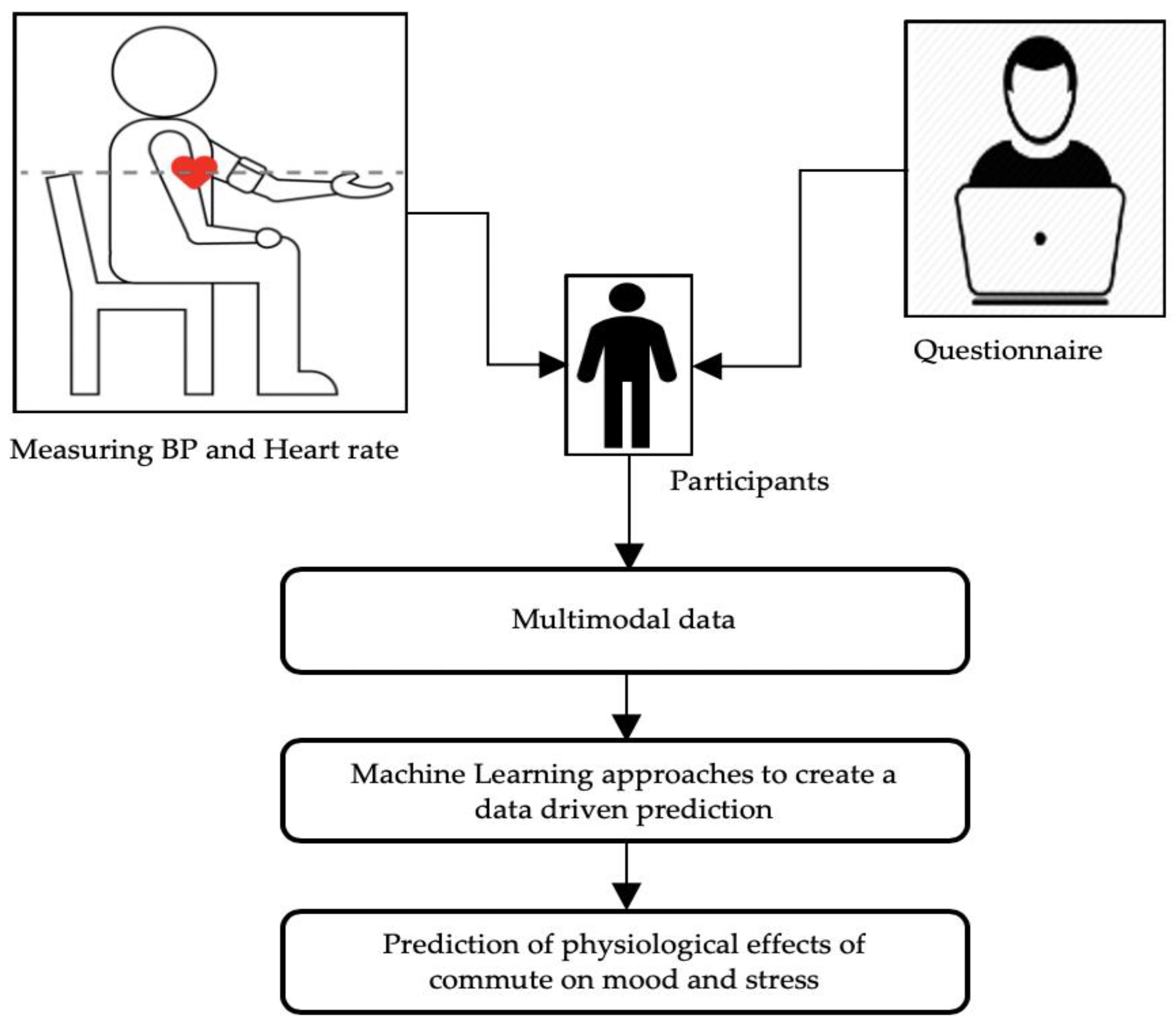
In this research, the data were collected from 16 participants who were employed and commuting regularly to work in London for five continuous working days. All participants signed an informed consent agreeing to participate in the research. Their participation in this study is entirely voluntary, and they were free to withdraw at any time during the research. They are from different parts of London, work in different places, and use different modes of commute. We collected two types of data—qualitative and quantitative—based on questionnaires (the Positive and Negative Affect Schedule [PANAS]) and bio-signals (BP and heart rate), respectively. Non-invasive wearable biosensor technology was employed to acquire the data from the research participants. The MySignals software-development platform was integrated into the system developed for the present research to measure blood pressure and heart rate. The normal BP measurement should be 120/80 mmHg systolic pressure over diastolic pressure. The BP monitor automatically measures the heart rate, where the normal reading should be between 60 and 100 beats per minute (bpm) [25]. Figure 1 shows the data collection process and study design.

After the BP and heart-rate readings of each participant were recorded, other subjective factors and parameters were taken into consideration, such as age, gender, smoking, height, alcohol intake, any medication intake, medical health, location, and weather temperature. The full dataset contains data for five days, with readings taken twice a day for each participant. High BP levels can represent fluctuations due to certain risk factors, such as high alcohol intake, high sodium intake, high protein intake, low calcium levels, as well as low potassium and magnesium intake [26].

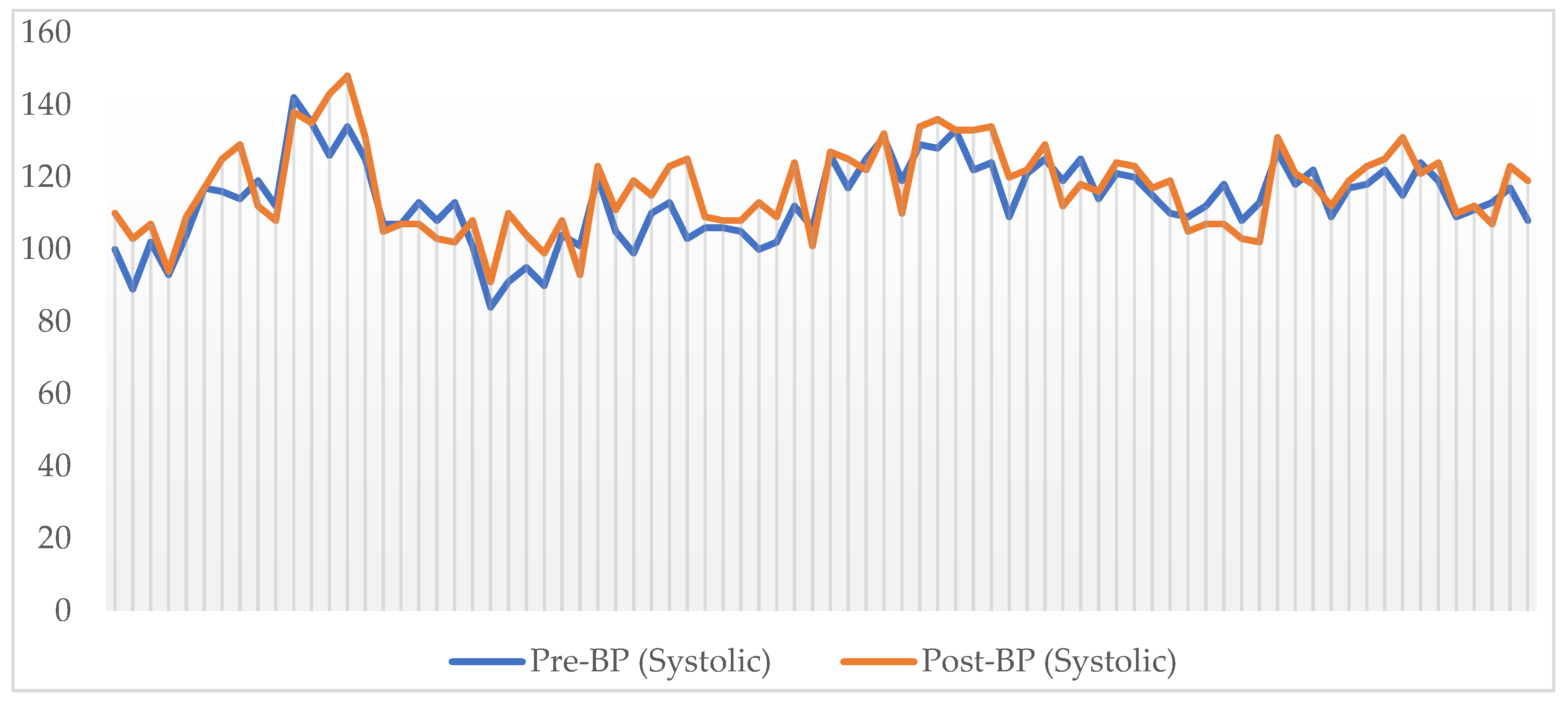
Blood pressure is the pressure of the blood in the arteries as it is pumped around the body by the heart. When our heart beats, it contracts and pushes blood through arteries to the rest of our body. This force creates pressure on the arteries. Blood pressure is recorded as two numbers: the systolic pressure (as the heart beats) over the diastolic pressure (as the heart relaxes between beats). In this research, we recorded the bio-signal (systolic pressure, diastolic pressure and heart rate) before and after the commute from the participants. Figure 2 illustrates a comparison of the pre-systolic pressure over the post-systolic pressure. As pre-systolic refers to systolic pressure recorded before the journey and post refers to systolic pressure recorded after the journey. 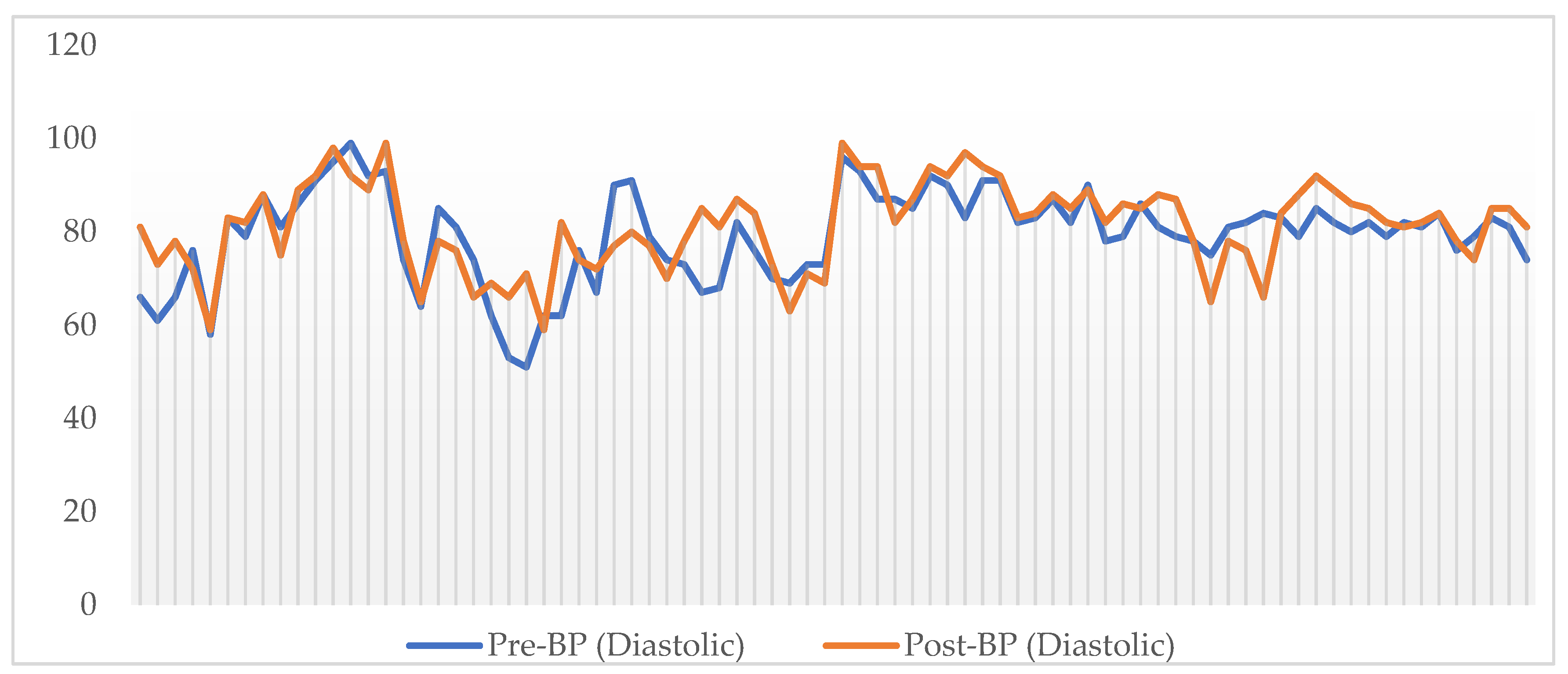Meanwhile, Figure 3 shows a comparison of diastolic pressure before and after the commute. Similarly, Figure 4 compares the recorded heart rate before and after the commute.

In this research, the data were divided into two categories. The first dataset contains only the relevant objective parameters (blood pressure and heart rate), and the second dataset includes all the subjective parameters such as age, height, weight, and alcohol consumption as well as the objective ones. Different machine-learning-based techniques are used in this study to objectively validate the proposed research hypotheses, which are as follows:

• Systolic BP will be higher in longer versus shorter commutes; and
• Objective bio-signals (heart rate, BP) for all participants will be higher post-commute than pre-commute.

We aim to analyse the biodata collected from the commuters in London and apply a machine-learning-based approach to predict the effect of a long commute on their heart rate and BP. The objectives of this research are thus as follows:

• to record biodata (BP and heart rate) of London commuters using non-invasive wearable technology; and
• to apply a machine-learning-based approach to predict the effect of a long commute on commuters’ heart rate and BP.

Questionnaires were used to gather the qualitative data, whereas the quantitative data are the biodata acquired from the participants via sensors. The research participants were asked to fill out a questionnaire form PANAS before and after commuting. The PANAS was developed in 1988 by researchers from the University of Minnesota and Southern Methodist University. Previous mood measures have shown correlations of variable strength between positive and negative affect, and these very measures are of questionable reliability and validity. Watson, Clark, and Tellegen developed the PANAS in an attempt to provide a better, purer measure of each of these dimensions [27]. The PANAS form contains a scale of different words that describe feelings and emotions that vary depending on the situation, environment, and weather [27]. It has been widely used as a self-report measure of effect in community and clinical contexts [28]. In the present study, this method is used to demonstrate effect related to commuting from a subjective point of view. The words employed in PANAS form describe how the participant feels at the moment of answering, such as expressing positive or negative affect before and after the journey [29]. In addition, we have a section in PANAS form for evaluation of the participant’s general stress levels; a participant needs to mention about any upcoming deadline at work, whether they slept well last night, anything annoying that occurred during a commute, and whether they considered yesterday to be a stressful day. In this questionnaire, the feelings and emotions were rated on a scale of 1 to 5, as illustrated in

Table 1. Positive and Negative Affect Schedule (PANAS) Scorecard [27].

1 Very Slightly or Not at All	2 A Little	3 Moderately		4 Quite a Bit	5 Extremely
1. Interested 2. Distressed 3. Excited 4. Upset 5. Strong 6. Guilty 7. Scared 8. Hostile 9. Enthusiastic 10. Proud			11. Irritable 12. Alert 13. Ashamed 14. Inspired 15. Nervous 16. Determined 17. Attentive 18. Jittery 19. Active 20. Afraid

.

In the beginning, all the participants went through the consent form and initial assessment questionnaire to check their suitability for the study. The participants recorded their feelings according to the proposed scale and rated them accordingly from 1 to 5, as shown in Table 1. The participants expressed their subjective feelings twice a day—at the beginning of their commute and the end. After filling out the questionnaire form, the participants started recording their BP and heart-rate readings. All the forms were submitted online and exported to the database. Other factors and parameters are taken into consideration included age, gender, smoking, height, alcohol intake, any medication intake, medical health, location, and weather temperature, and all these data were also exported to the database.

To apply the relevant effective techniques to the data, the data first needed to be pre-processed into the training and testing data for each of the techniques to test the hypotheses. All the values of the parameters in the dataset are in numerical form. In this experiment, two datasets were created for each hypothesis. In the first dataset, only the main parameters related to the hypothesis were included so that we could determine the pure effect of commuting on heart rate and BP. Similarly, for the second dataset, we included the main parameters plus all other parameters collected from the participants. From the second dataset, we can identify the effect of other parameters on heart rate and BP.

For the first hypothesis, the dataset was divided into two subsets. The first one contained the main parameters, such as BP, heart-rate readings (pre- and post-commute), and the duration of the commute in minutes. The second dataset included the main parameters (BP, heart-rate readings [pre- and post-commute] and duration of the commute in minutes) along with the other parameters, such as age, weight, height, smoking, alcohol intake, and temperature according to the weather report in the morning.

Similarly, for the second hypothesis, the dataset was divided into two subsets: the first one with BP and heart-rate readings (pre- and post-commute), and the second one with all parameters (i.e., BP, heart-rate readings [pre- and post-commute], duration of the commute in minutes, age, weight, height, smoking, alcohol intake, and temperature according to the weather report in the morning).

4. Implementation

We developed a machine-learning approach for the implementation and execution of the dataset analysis. Machine learning-based techniques were implemented to create an effective model, and different patterns and training algorithms were created to optimise the performance. The analysis was conducted by treating the data with each technique to obtain outputs that could then be compared in light of the hypotheses of this study. The data were processed for the input and target files and loaded into the software either by importing them from the system or loading them manually from the workspace.

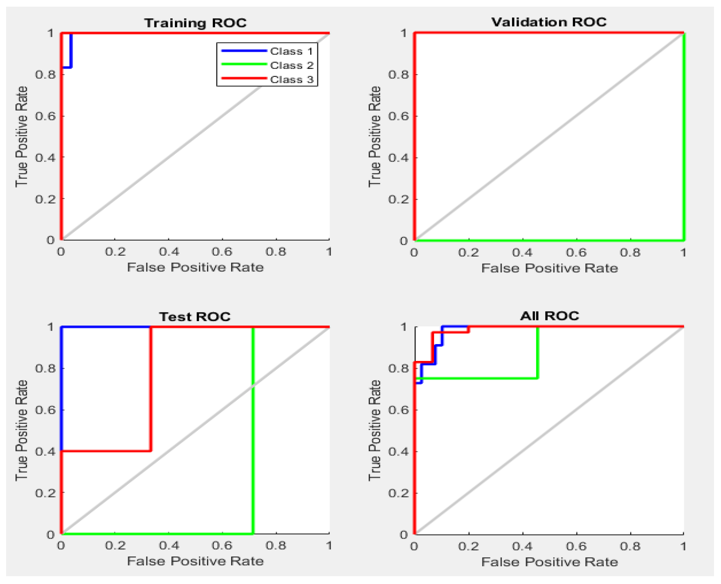
Model performance was evaluated using widely applied statistics, namely the area under the receiver-operator characteristics (ROC) curve or AUC statistic. The area under the ROC curve (AUC) has been used as a criterion to measure the performance of the classification algorithms even if the training data embraces an unbalanced class distribution and cost-sensitiveness [30]. In each class, the ROC curve applies the threshold values to the output values so that for each threshold, the true-positive ratio (TPR) and the false-positive ratio (FPR) values are simplified. 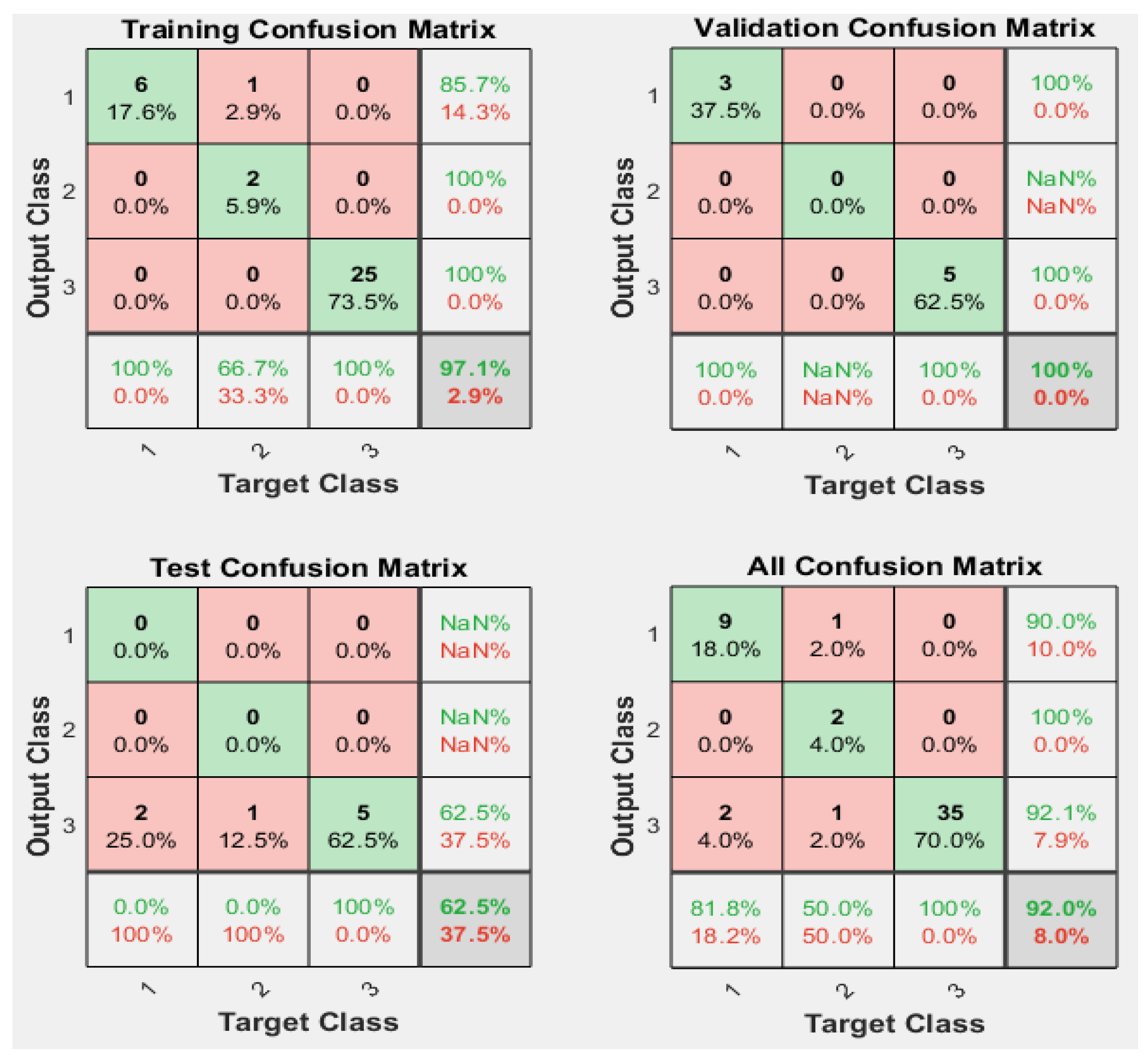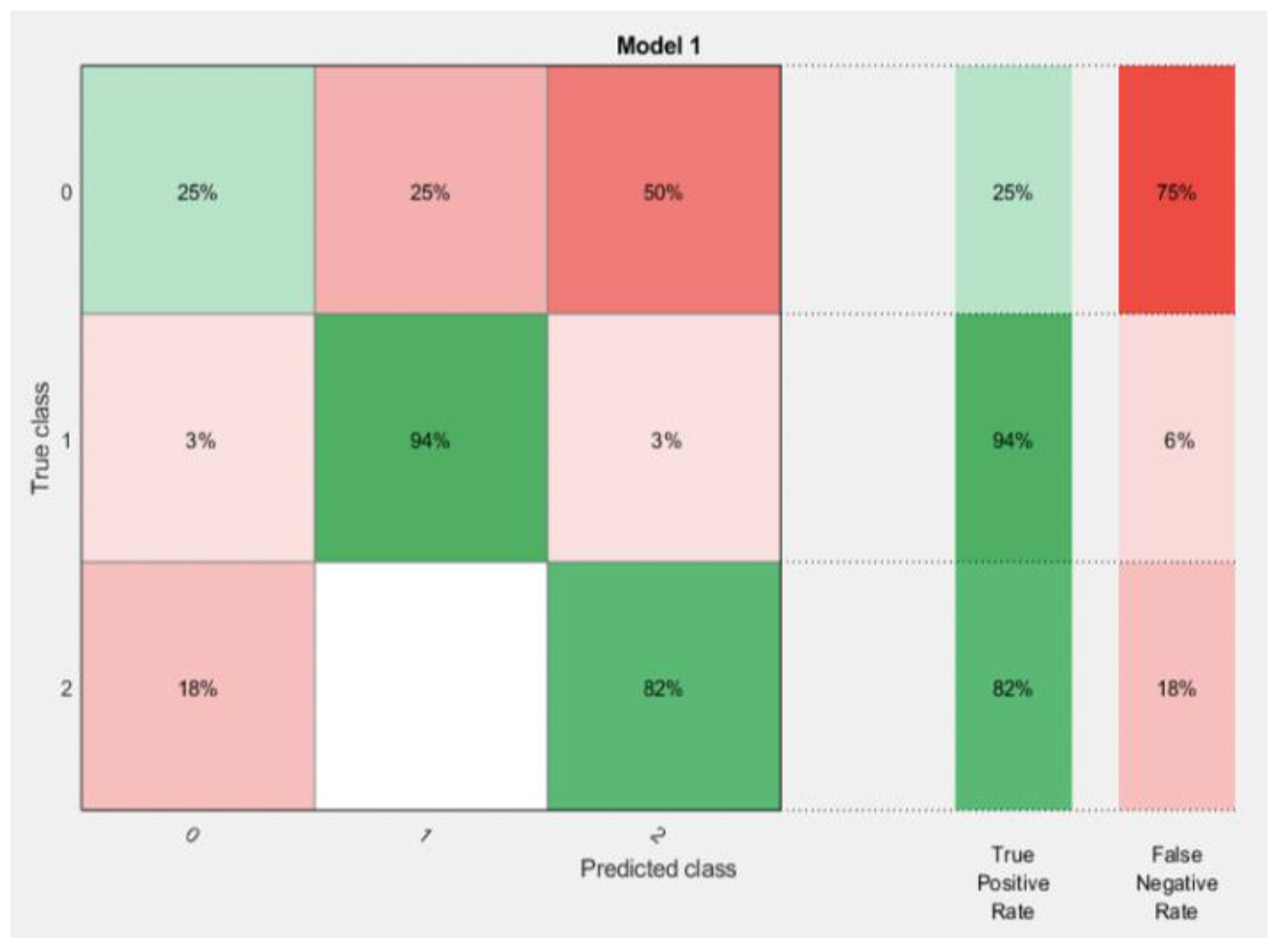This also represents the specificity and sensitivity of the data based on the predictions and observations carried out on the model throughout the training process of the model [31]. The confusion matrix measures and displays the accuracy of a classification model or a training model by comparing both the actual class and predicted class values. It is used to describe the efficiency of a classifier. It is critical for supervised learning in the field of machine learning [32].

To the relevant techniques to the data, the data must first be pre-processed to serve as training and testing data for each of the techniques to confirm the hypotheses. The data were divided into input data and target data. The input data are the values of the parameters from the dataset, and the target data were prepared by comparing the pre- and post-commute values from the data in the form of the numerical values 0, 1, and 2 for all the techniques. If the pre- and post-commute values are the same, then the target value is 0. If the pre-commute value is lower than the post-commute value, then the target value is 1. Finally, if the post-commute value is lower than the pre-commute value, then the target value is 2. In the feed-forward neural network technique, the target data value accepts binary values only. Therefore, the target data values for this technique were prepared in the form of a logical matrix with values of 0 and 1 only.

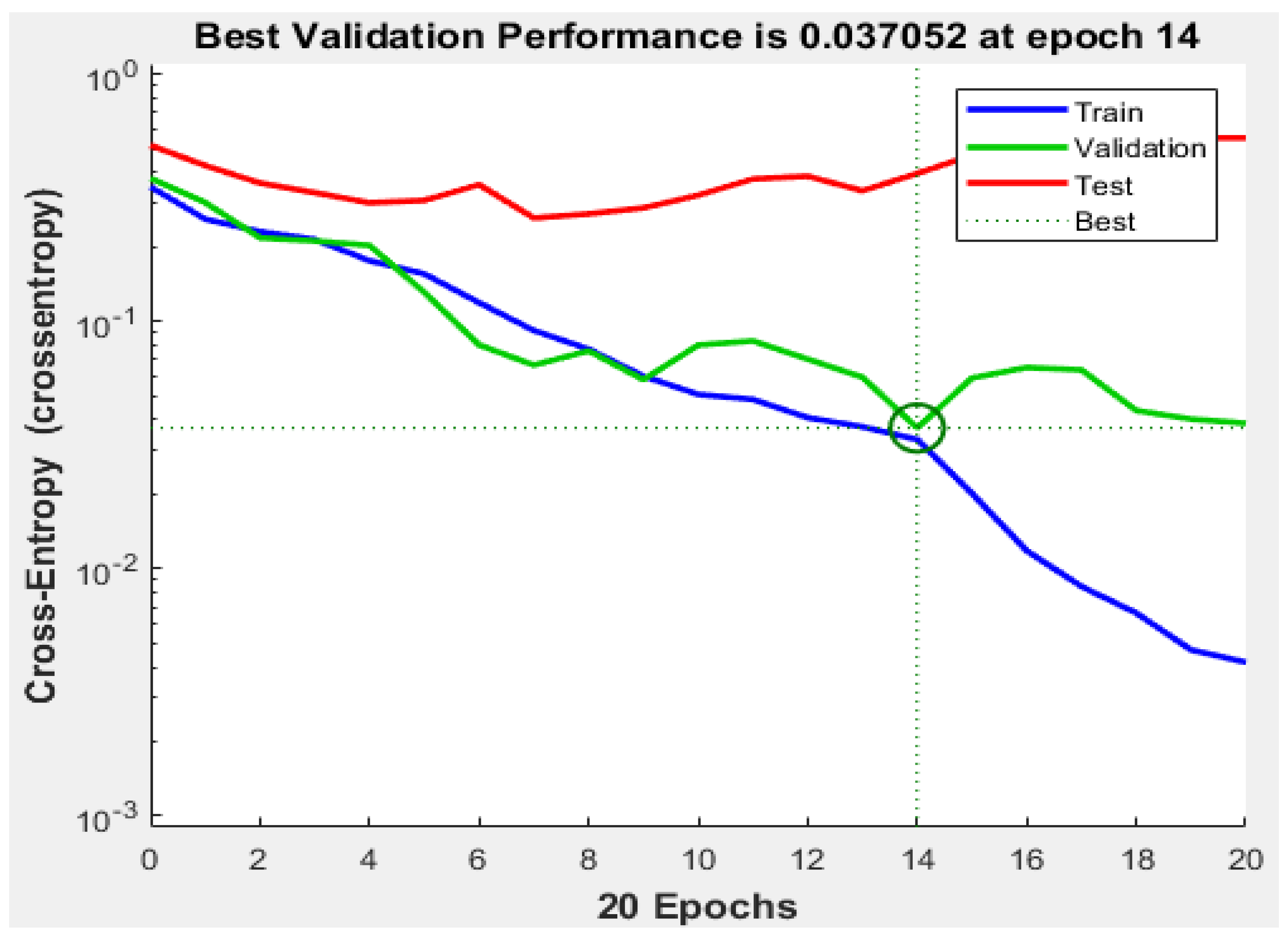
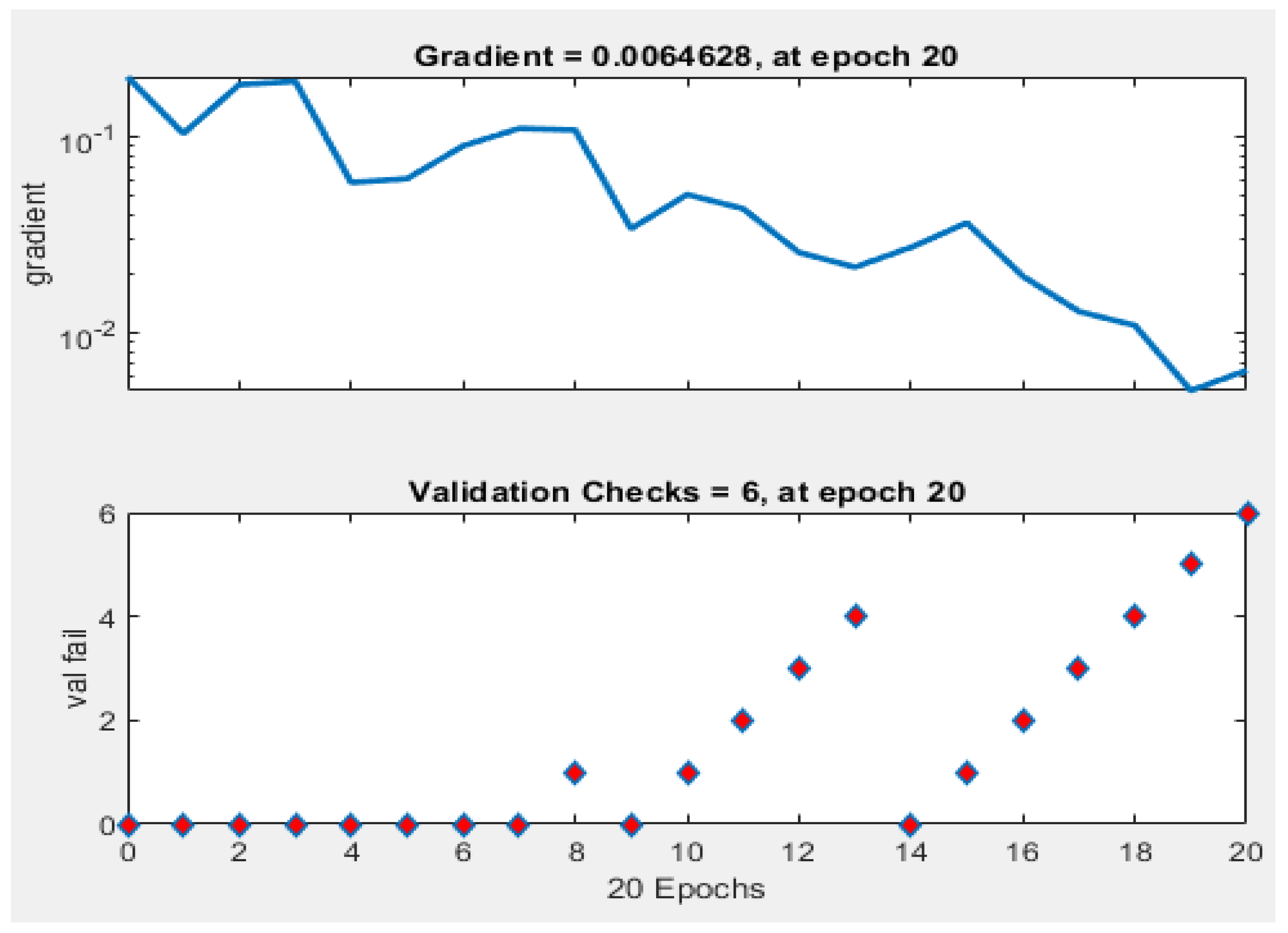
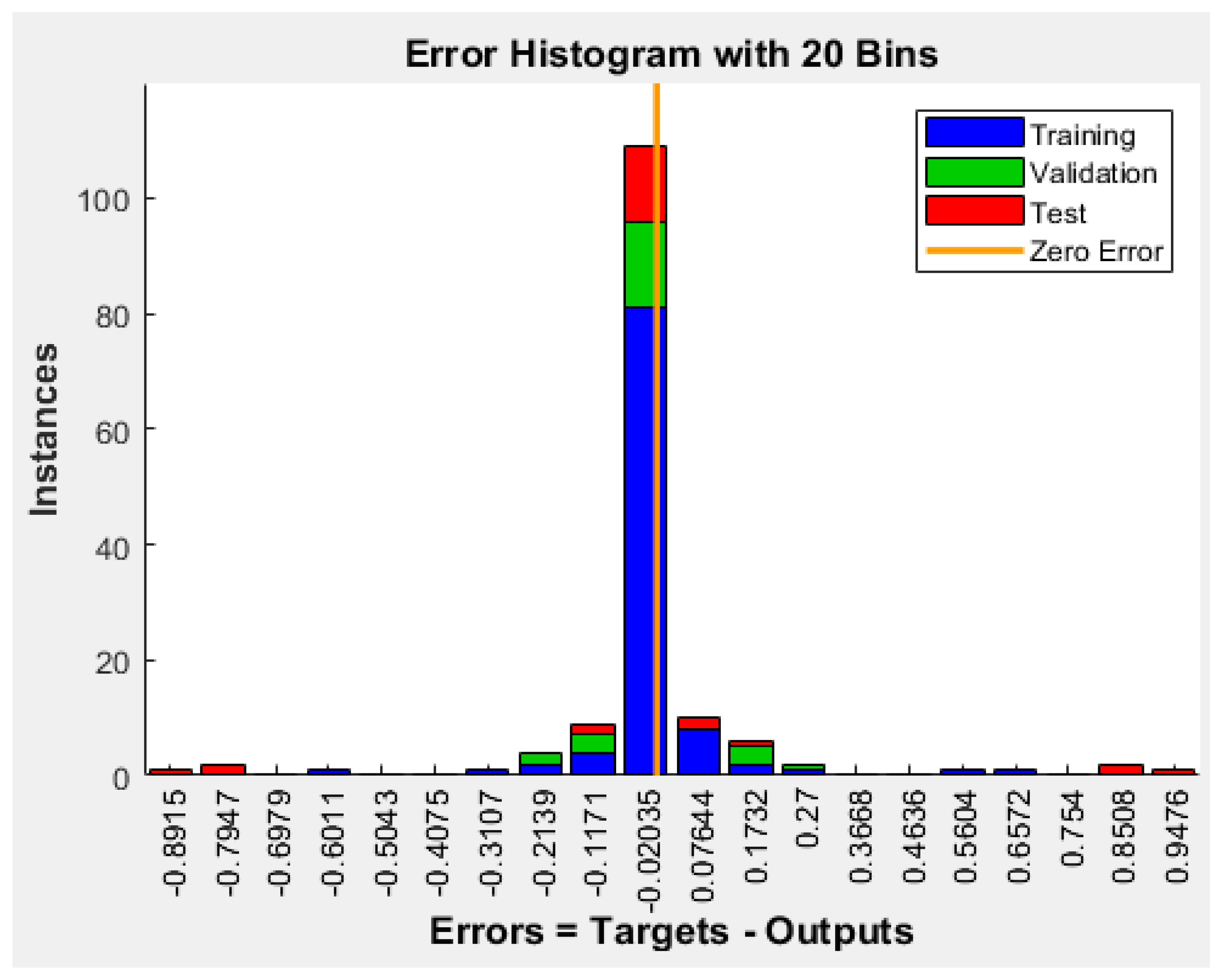
For each technique, the first input dataset and the target data were loaded into the workspace of the model. When the neural network pattern recognition application was opened, the datasets were then selected, and a training sample size of 70%, a validation sample size of 15%, and a testing sample size of 15% were selected under the training process. When the training started, the performance, training state, error histogram, confusion matrix, and ROC curve were plotted based on the data.

5. Results and Discussion

5.1. Validation of the First Hypothesis

The following three techniques were used to validate the first hypothesis, namely that “Systolic BP will be higher in longer commutes than in shorter commutes”:

5.1.1. Feed-Forward Neural Network

The feed-forward neural network is one of the simplest and most popular among the wide range of ANNs. It is an artificial neuron that is made up of linear combinations of weighted sums of the inputs as the ANN contains an input layer, hidden neuron layer, and output layer [16]. Any information inserted into this network flows linearly in a forward, one-way direction from the input layer through the hidden layer and then towards the output layer. The size of the training dataset was previously set to 70% by default by the application, and the validation and testing data sizes were set manually. The validation data and the testing data were set to equal sizes of 15% each to optimise the results. One of the major challenges in the design of a neural network is the fixation of hidden neurons with minimal error and highest accuracy. The number of hidden neurons was set to 10 to the network to perform well during training. The neural network training toolbox allows training using custom datasets and plots the confusion matrix and the ROC curve, respectively. The data were prepared via the training of the neural networks and the classifier models. The dataset was partitioned into two datasets with the following parameters: one with only the relevant parameters and the other with all the parameters. The inputs and targets were loaded and the hidden layer size was set to 10. The data were then divided into 70% training data, 15% validation data, and 15% testing data. The training algorithm used was the scaled conjugate gradient backpropagation method. The performance of the neural network was evaluated by calculating the errors using loss functions of cross-entropy while adjusting the weights and updating the bias by using the scaled conjugate gradient training algorithm. The neural network training performance for a total of 20 epochs was plotted, and the validation performance was plotted based on the simplified error values against the number of iterations or training epochs, as shown in Figure 5 below.

The neural network training state was evaluated and plotted by training the whole network based on the total number of records. The state depends upon the training function that was used to plot the network, which here is the scaled conjugate gradient function, as shown in Figure 6.

Figure 7 below presents an error histogram, which is a plot of a graph of a histogram of error values. This histogram represents any number of errors that occurred during the training of the model or the neural network between target values and predicted values after training a feed-forward neural network. As these error values indicate how the predicted values differ from the target values, they can be negative. The bins are the number of vertical bars on the graph. The total error range is divided into 20 smaller bins here. An error histogram of the feed-forward neural network is shown in Figure 7 below.

The confusion matrix in Figure 8 displays the accuracy of the feed-forward neural network by comparing the actual and predicted classes. The overall accuracy obtained for this model was 92% when the network was trained successfully. The model predicted 35 of the predicted values were found correct out of 35 to have increased just equal to the actual values, as per the assumed hypothesis. Similarly, for the second class, two values were misclassified out of 11, and in the third class, two values were misclassified out of four. The overall accuracy for this classifier is illustrated in Figure 8 below.

The ROC curve was plotted with all the iterations—all training, testing, and validating datasets and also with the whole dataset—and the accuracy was classified according to the training with the data in the network, as shown in Figure 9.

5.1.2. Linear Discriminant Analysis

Generally, this technique is considered for operations such as classification, regression, statistical analysis, and pattern recognition. As mentioned above, in this study, two datasets were compiled: one with the main parameters (BP and heartbeat) and the other with all the parameters collected from the participants, including the main parameters as well. The first dataset, with its input parameters and target data, was loaded into one file in the workspace.

Firstly, the classifier model was trained via a fivefold cross-validation method, which helps to protect against the overfitting of data or any noisy data. This training was successfully conducted for the first input data using the cross-validation method and no validation. After the model was trained, the accuracy obtained was 86% with validation and 92% without validation. When training was conducted with the second dataset, we obtained an accuracy level of 80% for the fivefold cross-validation and 94% without validation. Better results for metrics such as the accuracy and the precision values were shown for both datasets when trained with the no validation method compared to the cross-validation method, as shown in the confusion matrices in Figure 10 and Figure 11 below.

The second dataset containing all the objective and subjective variables was divided into the input or predictor variables and target or response variables when trained a second time via the fivefold cross-validation method. An accuracy level of 80% was obtained. In the confusion matrix shown in Figure 12 below, the TPR is 94% and the FNR is 100%, whereas the positive predicted value rate is 94% and the false discovery rate is 100%.

In the second dataset, the input predictor variables and the target response variables, when trained with no validation method, obtained a total accuracy level of 94%. In the confusion matrix in Figure 13, the TPR is 100%, and the FNR is 50%.

5.1.3. Decision Tree Technique

A decision tree is a supervised machine-learning technique for creating a structured tree with the help of the training data of a trained classifier model. It is also known as a predictive model because it can conduct mapping from observations about the dataset or any parameters or predictor variables by comparing them with the target or response variables. During the training of the classifier model, the first dataset was imported with the relevant parameters, which are the predictor variables, including the target data, which are the response variables to compare with the output of the classifier model. Afterwards, the fivefold cross-validation method has been employed to protect against the overfitting of data.

The confusion matrix was plotted against TPRs, FNRs, positive predictive values, false discovery rates, and the total number of observations against true classes and the predicted class values. The first dataset of input predictor variables and the target response variables, when trained via the cross-validation method, obtained a total accuracy of 76% overall. In the confusion matrix, for the predicted values, 3 predicted values were misclassified as decreased instead of increased, while just 5 predicted values were misclassified as increased instead of decreased. The TPR was 91%, and the FNR was 100%; however, the positive predicted value rate was 80%, and the false discovery rate was found to be 40%.

The same first dataset as before was used, which was comprised of input predictor variables and target response variables. When trained with no validation method, a higher accuracy of 90% was obtained. In the confusion matrix, 34 of the predicted values were found to be correct out of 35 to have increased just closer to the actual values, as per the assumed hypothesis. In the second class, three values were misclassified out of 11, and in the third class, one value was misclassified out of four. The TPR was 97%, which is higher than the validated trained model, and the FNR was 25%; however, the positive predicted value rate was 94%, and the false discovery rate was found to be 40%.

The second dataset including all the subjective and objective parameters was also used to train the classifier model using both validation methods. The target data values, or response variables, were in the form of 0 s, 1 s, and 2 s. In the target data, 0 means “the same”, 1 indicates an increased systolic BP, and 2 indicates decreased systolic BP readings, as required to test the hypothesis. When the model was trained, the accuracy obtained was 76% with the cross-validation method. The confusion matrix and ROC curve were plotted per data. The same first dataset as before was used, which was comprised of the input predictor variables and the target response variables. When the model was trained with no validation method, a higher accuracy of 90% was obtained. Similarly, for the second dataset, we obtained 99% accuracy for both the fivefold cross-validation and no validation cases.

5.1.4. Comparison of Performance of Artificial Intelligence Techniques Using Confusion Matrices

In this research, for all of the techniques applied to the data, a confusion matrix was plotted against the TPRs, FNRs, positive predictive values, false discovery rates, and the total number of observations against the true classes and the predicted class values. The results in

Table 2. Comparison of the confusion matrix for different artificial intelligence techniques for the first hypothesis (same: I, increase: II, decrease: III).

AI Technique	Dataset	Validation	Predicted Class (%)			Misclassification (%)
			I	II	III
Feed-forward neural network	First	No validation	18%	70%	4%	8%
	Second	No Validation	20%	70%	4%	6%
Linear Discriminant Analysis	First	5-fold cross-validation	2%	66%	18%	14%
		No Validation	4%	68%	20%	8%
	Second	5-fold cross-validation	0%	66%	14%	20%
		No validation	4%	70%	20%	6%
Decision Tree	First	5-fold cross-validation	0%	64%	12%	24%
		No validation	6%	68%	16%	10%
	Second	5-fold cross-validation	8%	70%	22%	0%
		No validation	8%	70%	22%	0%

show the accuracy levels of all the classifiers by comparing their actual and predicted classes. The feed-forward neural network exhibited the least misclassification of all the techniques. In Table 2, I represents that the value of the bio-parameter remained the same pre- and post-commute, II represents an increase from pre- to post-commute, and III represents a decrease in the value of the bio-parameter post-commute.

The learning performance of the feed-forward neural network was shown to be much better than that of other techniques.

Table 3. Comparison of different AI techniques with accuracy for the first hypothesis.

Technique	Dataset	Validation	Accuracy
Feed-forward neural network	First	No validation	92%
	Second	No validation	94%
Linear discriminant	First	5-fold cross-validation	86%
		No validation	92%
	Second	5-fold cross-validation	80%
		No validation	94%
Decision tree	First	5-fold cross-validation	76%
		No validation	90%
	Second	5-fold cross-validation	99%
		No validation	99%

below shows the different artificial intelligence techniques used along with their accuracy levels for the first hypothesis: “Systolic BP will be higher in longer commutes versus shorter commutes”.

Figure 14 shows comparisons of the different AI techniques used to examine the first hypothesis with their accuracy for the first and second datasets.

5.2. Validating the Second Hypothesis

Similarly, for the second hypothesis, “The objective bio-signals (heart rate, BP) for all participants will be higher post-commute than pre-commute”, we used the following three AI techniques:

5.2.1. Recurrent Neural Network

As mentioned above, a recurrent neural network is a type of neural network where the yields from past progress are a kind of nourishment that contributes to present progress. In traditional neural systems, every one of the data sources and yields is free of one another. However, for example, in cases when it is required to anticipate the next expression in a sentence, the past words are required and, consequently, there is a need to recall them. To deal with such cases, the RNN was developed, as it can explain such issues with the assistance of a “hidden layer”. This layer is the principal and most significant component of an RNN, which recalls certain data about a grouping. In applying this technique, we used the training function TRAINLM, LEARNGD for adaption learning; the performance function was given as the mean square error (MSE); the number of layers was selected as two; the properties were selected as Layer 1; the number of neurons given was 10, and the transfer function was the TANSIG technique, which was named after the hyperbolic tangent. The accuracy for the first dataset was 72%, and for the second, it was 62%.

5.2.2. Support Vector Machine

An SVM is a supervised machine-learning algorithm that can be used for classification or regression problems. It uses a technique called the kernel trick to transform the data, and then, based on these transformations, it finds an optimal boundary between the possible outputs. Simply put, it does some extremely complex data transformations and then figures out how to separate the data based on the labels or outputs that have been defined. The popularity of this technique is due to its capability of doing both classification and regression. There are different types of SVM techniques available, namely linear SVM, quadratic SVM, cubic SVM, fine Gaussian SVM, medium Gaussian SVM, and coarse Gaussian SVM. After training all the SVM techniques, we obtained 86.0% accuracy for linear SVM and quadratic SVM in the BP-systolic case. For the second dataset, linear SVM and fine Gaussian SVM obtained the same level of accuracy.

5.2.3. K-Nearest Neighbours

In this algorithm, k-means clustering creates k groups from a set of objects to increase the similarity among the members of each group. It is a popular cluster analysis technique for exploring datasets. Cluster analysis is a family of algorithms designed to form groups such that the group members are more similar to one another than to non-group members. It is popular because of its simplicity, which means that it is generally fast and more efficient than other algorithms, especially over large datasets. For systolic BP, we obtained accuracy rates of 66% and 65% for the first and second datasets, respectively. Similarly, for diastolic BP, we obtained 78% accuracy for both datasets. Finally, we obtained 68% accuracy for both datasets for heart rate.

5.2.4. Comparison of Performance of Artificial Intelligence Techniques Using a Confusion Matrix

The confusion matrix is used to visualise the accuracy of all the classifiers by comparing the actual and predicted classes, as shown in

Table 4. Comparison of confusion matrix for different AI techniques for the second hypothesis (same: I, increase: II, decrease: III). BP: blood pressure.

AI Technique	Bio-Parameter	Dataset	Predicted Class			Misclassification (%)
			I	II	III
Support Vector Machine	Systolic-BP	First	0%	56%	30%	14%
		Second	0%	56%	30%	14%
	Diastolic-BP	First	13%	42%	8%	37%
		Second	2%	64%	12%	22%
	Heart rate	First	0%	66%	22%	12%
		Second	0%	62%	16%	22%
Recurrent Neural Network	Systolic-BP	First	0%	72%	0%	28%
		Second	0%	54%	8%	38%
	Diastolic-BP	First	0%	72%	0%	28%
		Second	0%	54%	8%	38%
	Heart rate	First	0%	72%	0%	28%
		Second	0%	54%	8%	38%
K-Nearest Neighbours	Systolic-BP	First	0%	62%	4%	34%
		Second	16%	48%	14%	42%
	Diastolic-BP	First	0%	72%	0%	28%
		Second	17%	55%	7%	21%
	Heart rate	First	0%	60%	8%	32%
		Second	0%	60%	8%	32%

below. In the table, the SVM exhibits the least misclassification compared to other techniques. In the Predicted Class columns, I represents the case in which the values of the bio-parameters stay the same post-commute, II represents an increase post-commute, and III represents a decrease in values of the bio-parameters post-commute.

Table 5. Artificial intelligence techniques with accuracy for the second hypothesis.

Technique	Dataset	Accuracy
		Systolic-BP	Diastolic-BP	Heart Rate
Support vector machine	First	86%	78%	88%
	Second	63%	77%	78%
K-nearest neighbours	First	66%	78%	68%
	Second	65%	78%	68%
Recurrent neural network	First	72%	72%	72%
	Second	62%	62%	72%

below shows the different artificial intelligence techniques used for commuting-effect prediction with the accuracy as obtained for the second hypothesis: “The objective bio-signals (heart rate, BP) for all participants will be higher post-commute than pre-commute”.

Figure 15 below shows different artificial intelligence techniques used for commuting-effect prediction with their accuracy for the second hypothesis.

5.3. PANAS Results

In this study, the participants were required to fill out the PANAS form before and after commuting. The form consists of different words that describe feeling and emotions [28] and is sensitive to fluctuations in mood.

Scoring Instructions

To score the positive affect, we added up the scores on lines 1, 3, 5, 9, 10, 12, 14, 16, 17, and 19 from Table 1. The scores on the PANAS Scorecard range anywhere from 10 to 50. Higher scores represent higher levels of positive affect. Similarly, to score the negative affect, we added up the scores on items 2, 4, 6, 7, 8, 11, 13, 15, 18, and 20 from Table 1. Again, the scores range anywhere from 10 to 50. Following the scoring instructions, we calculated the positive and negative affect pre- and post-commute. Then, we calculated the average of pre-positive affect, pre-negative affect, post-positive affect, and post-negative affect for all of the participants.

Table 6. Average of positive and negative affect from PANAS.

Avg Pre-Positive Affect	Avg Post-Positive Affect	Avg Pre-Negative Affect	Avg Post-Negative Affect
33.75	30.88	12.9	14.92

below shows the values for average positive and negative affect before and after commuting from the PANAS Scorecard.

From Table 6, we can see that the positive affect of pre-commute is higher than post-commute, which signifies that the participants’ feelings and emotions were more positive before the commute. Similarly, the negative affect score is lower pre-commute than post-commute, signifying that the participants were more stressed, or their feelings were more negative after their commute.

Similarly, based on the results obtained using the PANAS, we found that positive affect was higher pre-commute, which indicates that the participants more positive or interested in going to work before the commute. Negative affect is higher after the commute, which indicates a less interested or stressed state post-commute.

When comparing the results obtained using both approaches, those obtained from the machine-learning-based approach matched the subjective results obtained from the PANAS.

In this research, blood pressure and heart rate are main parameters to predict the stress level. In addition, we collected the parameters such as age, gender, smoking, height, alcohol intake, any medication intake, medical health, location, weather (temperature). We have also added the section in PANAS form for evaluation of the participant’s general stress levels; a participant needs to mention about any upcoming deadline at work, whether they slept well last night, anything annoying that occurred during a commute, and whether they considered yesterday to be a stressful day. In this research, the data were collected from participants who were employed and commuting regularly to work in London for five continuous working days. Some of the issues included the participants being from different part of London, having different cultural backgrounds, and being interviewed on different days. These things might slightly challenge model assumptions.

6. Conclusions

In this study, we developed an intelligent model based on different machine-learning approaches to predict the effect of commuting on heart rate and BP. Further, we used questionnaires (the PANAS) to demonstrate the impact of commuting on effect from a subjective point of view. When we applied the machine-learning based model, whether the commute duration was short or long, it was noticed that the systolic pressure was usually higher post-commute than pre-commute one, and we found the objective bio-signals (heart rate and BP) to be higher post-commute than pre-commute one. BP and heart rate are positively correlated to mood and stress. Based on this machine-learning approach, we were able to determine the participants’ level of stress after commuting.

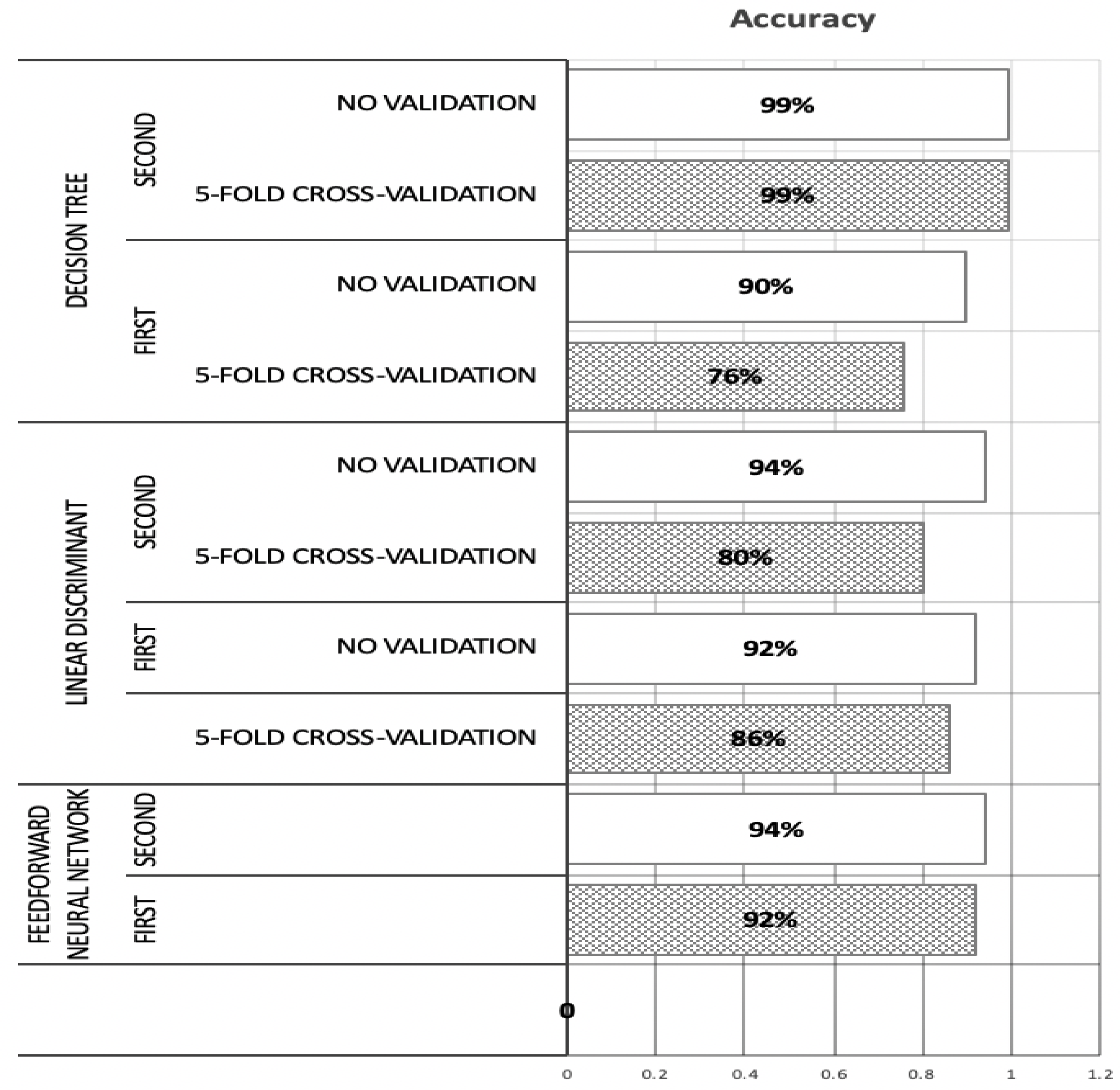
A comprehensive experiment was conducted to achieve the best structure for the feed-forward neural network, which suited the processed datasets. An accuracy level of 92% was obtained for the first dataset, which included only the main bio-signals, while an accuracy level of 94% was achieved for the second dataset, which included the main bio-parameters plus other subjective parameters collected from the participants. This increase in accuracy shows that the neural network was able to achieve better performance with the dataset containing both quantitative and qualitative parameters. The quantitative results confirmed the proposed hypothesis, which assumed that the systolic BP would be higher for longer commutes versus shorter ones, as it was found that the post-commute readings for systolic BP were higher, irrespective of the duration of the commute. Systolic BP was normally higher for shorter commutes than for longer ones.

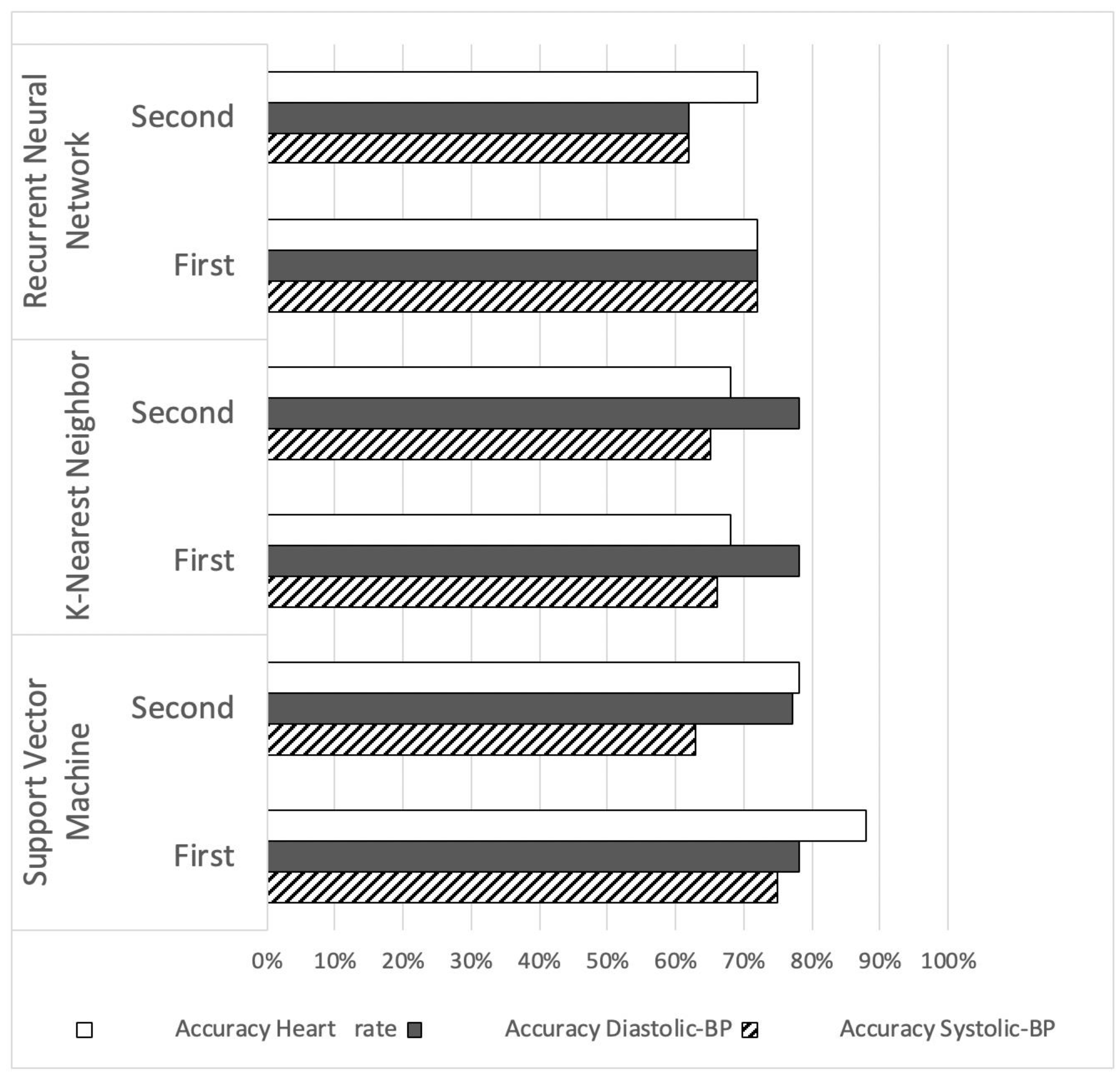
Similarly, the results achieved by the fused machine-learning techniques confirmed the second hypothesis, which assumed that the bio-parameters (diastolic BP and heart rate) would be higher post-commute than pre-commute. The processed dataset was also partitioned into two datasets of parameters, one with only the relevant bio-parameters and the other with all the quantitative and qualitative parameters. In addition to the objective evaluation based on the machine-learning techniques, we used the PANAS survey, which has been widely utilised as a self-report measure of effect in both community and clinical contexts. From the PANAS results, it was determined that the positive affect of the participants was higher pre-commute than post-commute, which indicates that the mood and emotional state of the participants were more positive before commuting. Similarly, the negative affect of the participants was higher post-commute than pre-commute, which indicates that the participants were more stressed after the commute.

This research study forms a core work that gives us the ability to find the effect of commuting on people who commute to work five days a week. In this research, participants from all over Greater London were involved. Our future work in this area will leverage innovative machine-learning-based approaches to predict and evaluate the effect of commuting on productivity in the workplace as well as to study the psychological and physiological effects of commuting.

References

1. Sano, A.; Picard, R.W. Stress recognition using wearable sensors and mobile phones. In Proceedings of the 2013 Humaine Association Conference on Affective Computing and Intelligent Interaction, Geneva, Switzerland, 2–5 September 2013; pp. 671–676. [Google Scholar]
2. Boonnithi, S.; Phongsuphap, S. Comparison of heart rate variability measures for mental stress detection. In Proceedings of the 2011 Computing in Cardiology, Hangzhou, China, 18–21 September 2011; pp. 85–88. [Google Scholar]
3. Vrijkotte, T.; van Doornen, L.; de Geus, E. Effects of work stress on ambulatory blood pressure, heart rate, and heart rate variability. Hypertension 2000, 35, 880–886. [Google Scholar] [CrossRef] [PubMed]
4. Pramanta, S.P.L.A.; Prihatmanto, A.S.; Park, M. A study on the stress identification using observed heartbeat data. In Proceedings of the 6th International Conference on System Engineering and Technology (ICSET), Bandung, Indonesia, 3–4 October 2016; pp. 149–152. [Google Scholar]
5. Being Sick of the Daily Commute Could Be Affecting Your Health. Available online: https://www.nhs.uk/news/lifestyle-and-exercise/being-sick-of-the-daily-commute-could-be-affecting-your-health/ (accessed on 8 June 2019).
6. Triantafyllidis, A.; Tsanas, A. Applications of Machine Learning in Real-Life Digital Health Interventions: Review of the Literature. J. Med. Internet Res. 2019, 21, e12286. [Google Scholar] [CrossRef] [PubMed] [Green Version]
7. Bhattarai, A.; Rus, V.; Dasgupta, D. Classification of clinical conditions: A case study on prediction of obesity and its co-morbidities. In Proceedings of the 10th International Conference on Intelligent Text Processing and Computational Linguistics (CICLING ’09), Mexico City, Mexico, 1–7 March 2009. [Google Scholar]
8. Pollettini, J.T.; Panico, S.R.; Daneluzzi, J.C.; Tinós, R.; Baranauskas, J.A.; Macedo, A.A. Using machine learning classifiers to assist healthcare-related decisions: Classification of electronic patient records. J. Med. Syst. 2012, 36, 3861–3874. [Google Scholar] [CrossRef] [PubMed]
9. Sharif, M.S.; Abbod, M.; Al-Bayatti, A.; Amira, A.; Alfakeeh, A.S.; Sanghera, B. An accurate ensemble classifier for medical volume analysis: Phantom and clinical PET study. IEEE Access 2020, 8, 37482–37494. [Google Scholar] [CrossRef]
10. Jung, Y.K.; Baek, H.C.; Soo, M.I.; Myoung, J.J.; Kim, I.Y.; Kim, S.I. Comparative study on artificial neural network with multiple regressions for continuous estimation of blood pressure. In Proceedings of the IEEE Engineering in Medicine and Biology 27th Annual Conference, Shanghai, China, 1–4 September 2005; pp. 6942–6945. [Google Scholar]
11. Sharif, M.S.; Amira, A. An intelligent system for PET tumour detection and quantification. In Proceedings of the 16th IEEE International Conference on Image Processing (ICIP), Cairo, Egypt, 7–10 November 2009; pp. 2625–2628. [Google Scholar]
12. Faraz, S.; Azhar Ali, S.S.; Hasan Adil, S. Machine learning and stress assessment: A review. In Proceedings of the 3rd International Conference on Emerging Trends in Engineering, Sciences and Technology (ICEEST), Karachi, Pakistan, 21–22 December 2018; pp. 1–4. [Google Scholar]
13. Zhang, B.; Ren, J.; Cheng, Y.; Wang, B.; Wei, Z. Health data driven on continuous blood pressure prediction based on gradient boosting decision tree algorithm. IEEE Access 2019, 7, 32423–32433. [Google Scholar] [CrossRef]
14. Sharif, M.S.; Abbod, M.; Amira, A. Neuro-fuzzy based approach for analysing 3D PET volume. In Proceedings of the IEEE International Conference on the Developments on eSystems Engineering (DeSE)—Special Session, Intelligent technologies on Cancer Research, Dubai, United Arab Emirates, 6–8 December 2011; pp. 158–163. [Google Scholar]
15. Obayya, M.; Abou-Chadi, F. Data fusion for heart diseases classification using multi-layer feed forward neural network. In Proceedings of the 2008 International Conference on Computer Engineering & Systems, Cairo, Egypt, 25–27 November 2008; pp. 67–70. [Google Scholar]
16. Samant, R.; Rao, S. Evaluation of artificial neural networks in prediction of essential hypertension. Int. J. Comput. Appl. 2013, 81, 34–38. [Google Scholar] [CrossRef]
17. Rajeswari, K.; Vaithiyanathan, V.; Neelakantan, T. Feature selection in ischemic heart disease identification using feed forward neural networks. Procedia Eng. 2012, 41, 1818–1823. [Google Scholar] [CrossRef] [Green Version]
18. Kendale, S.; Kulkarni, P.; Rosenberg, A.; Wang, J. Supervised machine-learning predictive analytics for prediction of postinduction hypotension. Anesthesiology 2018, 29, 675–688. [Google Scholar] [CrossRef] [PubMed]
19. Argerich, S.; Herrera, S.; Benito, S.; Giraldo, B.F. Evaluation of periodic breathing in respiratory flow signal of elderly patients using SVM and linear discriminant analysis. In Proceedings of the 2016 38th Annual International Conference of the IEEE Engineering in Medicine and Biology Society (EMBC), Orlando, FL, USA, 16–12 August 2016; pp. 4276–4279. [Google Scholar]
20. Kadi, I.; Idri, A. A decision tree-based approach for cardiovascular dysautonomias diagnosis: A case study. In Proceedings of the 2015 IEEE Symposium Series on Computational Intelligence, Cape Town, South Africa, 7–10 December 2015; pp. 816–823. [Google Scholar]
21. Kampouraki, A.; Manis, G.; Nikou, C. Heartbeat time series classification with support vector machines. IEEE Trans. Inf. Technol. Biomed. 2009, 13, 512–518. [Google Scholar] [CrossRef] [PubMed]
22. Liang, B.; Duan, K.; Xie, Q.; Atef, M.; Qian, Z.; Wang, G.; Lian, Y. Live demonstration: A support vector machine based hardware platform for blood pressure prediction. In Proceedings of the 2016 IEEE Biomedical Circuits and Systems Conference (BioCAS), Shanghai, China, 17–19 October 2016; p. 130. [Google Scholar]
23. Rojo-Alvarez, J.; Barquero-Perez, O.; Mora-Jimenez, I.; Everss, E.; Rodriguez-Gonzalez, A.; Garcia-Alberola, A. Heart rate turbulence denoising using support vector machines. IEEE Trans. Biomed. Eng. 2009, 56, 310–319. [Google Scholar] [CrossRef] [PubMed]
24. Kao, W.; Wei, C.; Liu, J.; Hsiao, P. Automatic heart sound analysis with short-time Fourier transform and support vector machines. In Proceedings of the 2009 52nd IEEE International Midwest Symposium on Circuits and Systems, Cancun, Mexico, 2–5 August 2009; pp. 188–191. [Google Scholar]
25. NHS. What is Blood Pressure? 2020. Available online: https://www.nhs.uk/common-health-questions/lifestyle/what-is-blood-pressure/ (accessed on 6 February 2019).
26. Bhaduri, A.; Bhaduri, A.; Bhaduri, A.; Mohapatra, P.K. Blood pressure modeling using statistical and computational intelligence approaches. In Proceedings of the 2009 IEEE International Advance Computing Conference, Patiala, India, 6–7 March 2009; pp. 1026–1030. [Google Scholar]
27. Watson, D.; Clark, L.; Tellegen, A. Development and validation of brief measures of positive and negative affect: The PANAS scales. J. Personal. Soc. Psychol. 1988, 54, 1063–1070. [Google Scholar] [CrossRef]
28. Merz, E.; Malcarne, V.; Roesch, S.; Ko, C.; Emerson, M.; Roma, V.; Sadler, G. Psychometric properties of Positive and Negative Affect Schedule (PANAS) original and short forms in an African American community sample. J. Affect. Disord. 2013, 151, 942–949. [Google Scholar] [CrossRef] [PubMed] [Green Version]
29. Positive Psychology. What is the Positive and Negative Affect Schedule? 2020. (PANAS). Available online: https://positivepsychology.com/positive-and-negative-affect-schedule-panas/ (accessed on 4 March 2020).
30. Zhang, X.; Jiang, C. Improved SVM for learning multi-class domains with ROC evaluation. In Proceedings of the 2007 International Conference on Machine Learning and Cybernetics, Hong Kong, China, 19–22 August 2007; pp. 2891–2896. [Google Scholar]
31. MathWorks. ROC–Receiver Operating Characteristic. Available online: https://uk.mathworks.com/help/ deeplearning/ref/roc.html (accessed on 6 February 2019).
32. George, R.M.; Mathew, D. Emotion Classification Using Machine Learning and Data Preprocessing approach on Tulu speech data. 2016. Available online: https://pdfs.semanticscholar.org/36d5/b79cd1b92138fc70175124c94a0890c263d9.pdf (accessed on 6 May 2019).
Figure 1. Data collection and study design.
Symmetry 12 00866 g001
Figure 2. Comparison of pre-systolic pressure and post-systolic pressure.
Symmetry 12 00866 g002
Figure 3. Comparison of pre-diastolic pressure and post-diastolic pressure.
Symmetry 12 00866 g003
Figure 4. Comparison of pre-heart rate and post-heart rate.
Symmetry 12 00866 g004
Figure 5. Performance plot for feed-forward network for the first dataset.
Symmetry 12 00866 g005
Figure 6. Training state plot for feed-forward network for the first dataset.
Symmetry 12 00866 g006
Figure 7. Error histogram for feed-forward neural network.
Symmetry 12 00866 g007
Figure 8. Confusion matrix for the feed-forward neural network.
Symmetry 12 00866 g008
Figure 9. Performance of feed-forward neural network using the receiver-operator characteristics (ROC) curve.
Symmetry 12 00866 g009
Figure 10. Accuracy of the linear discriminant for the first dataset with validation.
Symmetry 12 00866 g010
Figure 11. Accuracy of the linear discriminant for the first dataset with no validation.
Symmetry 12 00866 g011
Figure 12. Accuracy of linear discriminant using confusion matrix for the second dataset with validation.
Symmetry 12 00866 g012
Figure 13. Accuracy of linear discriminant using the confusion for the second dataset with no validation.
Symmetry 12 00866 g013
Figure 14. Classification accuracy for artificial intelligence techniques for the first hypothesis.
Symmetry 12 00866 g014
Figure 15. Classification accuracy for artificial intelligence techniques for second hypothesis.
Symmetry 12 00866 g015