Contextual Modulation in Mammalian Neocortex is Asymmetric

Abstract

Neural systems are composed of many local processors that generate an output given their many inputs as specified by a transfer function. This paper studies a transfer function that is fundamentally asymmetric and builds on multi-site intracellular recordings indicating that some neocortical pyramidal cells can function as context-sensitive two-point processors in which some inputs modulate the strength with which they transmit information about other inputs. Learning and processing at the level of the local processor can then be guided by the context of activity in the system as a whole without corrupting the message that the local processor transmits. We use a recent advance in the foundations of information theory to compare the properties of this modulatory transfer function with that of the simple arithmetic operators. This advance enables the information transmitted by processors with two distinct inputs to be decomposed into those components unique to each input, that shared between the two inputs, and that which depends on both though it is in neither, i.e., synergy. We show that contextual modulation is fundamentally asymmetric, contrasts with all four simple arithmetic operators, can take various forms, and can occur together with the anatomical asymmetry that defines pyramidal neurons in mammalian neocortex.

1. Introduction

Biological and artificial neural systems are composed of many local processors, such as neurons or microcircuits, that are interconnected to form various network architectures in which the connections are adaptable via various learning algorithms. The architectures of mammalian neocortex, and of the artificial nets trained by deep learning, have several hierarchical levels of abstraction. In mammalian neocortex there are also feedback and lateral connections within and between different levels of abstraction. The information processing capabilities of neural systems do not depend only on their learning algorithms and architectures, however. They also depend upon the transfer functions that relate each local processor’s outputs to its inputs. These transfer functions are often described in terms of the simple arithmetic operators, e.g., [1,2]. Distinguishing them on that basis can be misleading, however, because real physiological operations are rarely, if ever, that simple.

In biological systems feedback and lateral connections can modulate transmission of feedforward information in various ways. There is ample evidence that modulatory interactions are widespread in mammalian neocortex [3,4,5,6]. Many very different forms of interaction have been called ‘modulatory’, however, and our concern here is with a particular kind of context-dependent form of modulation for which there is direct evidence at the intracellular level. 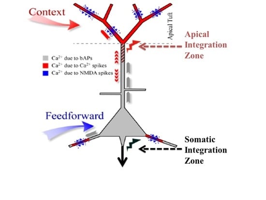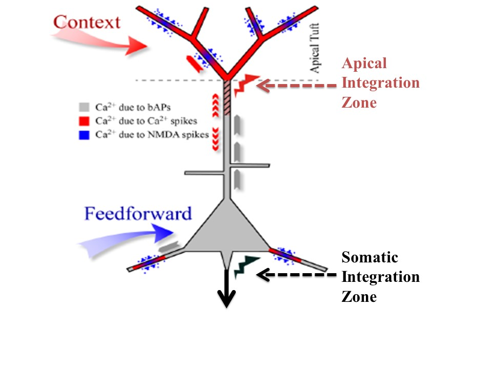This evidence calls into question the common assumption that, from a computational point of view, neurons in general can be adequately thought of as being leaky integrate-and-fire point neurons [7]. They are called point neurons because it is assumed that all their inputs are integrated at the soma to compute the value of a single variable about which information is then transmitted to downstream cells. Though that assumption may indeed be adequate for many kinds of neuron it is not adequate for some principal pyramidal neurons in the cerebral cortex. There is now clear evidence from multi-site intracellular recordings for the existence of a second site of integration near the top of the apical trunk of some neocortical pyramidal cells, such as those in layer 5B. We refer to this second point of integration as the apical integration zone, but it is also sometimes referred to as the ‘nexus’. This second point of integration may be of crucial relevance to our understanding of contextual modulation in the neocortex because anatomical and physiological evidence suggests that activation of the apical integration zone serves as a context that modulates transmission of information about the integrated basal input. The analyses reported here add to our understanding of that theoretical possibility.

We have reviewed the anatomical, physiological, and computational evidence for context-sensitive two-point processors at length elsewhere, as noted below [6] but give a summary here. Evidence for an intracellular mechanism that uses apical input to modulate neuronal output was first reported several years ago [8,9,10,11], though much remains to be learned about the far-reaching implications of such mechanisms. In vitro studies of rat somatosensory cortex show that in addition to the somatic sodium spike initiation zone that triggers axonal action potentials, layer 5 pyramidal cells have a zone of integration just below the main bifurcation point near the top of the apical trunk. If it receives adequate depolarization from the tuft dendrites and a backpropagated spike from the somatic sodium spike initiation zone it triggers calcium spikes that propagate to the soma [8], where it has a strong modulatory effect on the cell’s response to weak basal inputs by converting a single axonal spike into a brief burst of from two to four spikes. Distal apical dendrites are well positioned to implement contextual modulation because they receive their inputs from a wide variety of sources, including non-specific thalamic nuclei, long-range descending pathways, and lateral pathways [9]. Being so remote from the soma, however, input to the apical tuft of layer 5 cells has little effect on output unless propagated to the soma by active dendritic currents. A consequence of this is that input to the tuft alone usually has little or no effect on axonal action potentials, which we assume to be a crucial distinctive property of contextual modulation.

Contextual modulation is of fundamental importance to basic cognitive functions such as perceptual organization, contextual disambiguation, and background suppression [6,12,13,14,15,16,17,18,19]. Many reviews show that selective attention also has modulatory effects (e.g., [20]). There are several hypotheses concerning the neuronal mechanisms by which such modulation may be achieved [21]. Some make use of the distinct anatomy and physiological functions of apical and basal inputs outlined above [22,23,24], and our focus is on the basic information processing properties of such context-sensitive two-point processors.

The central goal of the work reported here is to use advanced forms of multivariate mutual information decomposition to analyze the information processing properties of such context-sensitive two-point processors and compare them with additive, subtractive, multiplicative and divisive interactions. It has been shown that artificial neural systems composed of such context-sensitive two-point neurons can learn to amplify or attenuate feedforward transmission within hierarchical architectures [25,26,27], but the full computational potential of such systems has not yet been adequately explored. Though the primary concern of this paper is biological, we frequently relate it to machine learning using artificial neural nets because that provides clear evidence on the computational capabilities of the biological processes inferred.

To explore the fundamental information processing capabilities of this form of asymmetric contextual modulation this paper compares it with the arithmetic transfer functions that have previously been used to interpret data on ‘neuronal arithmetic’ [1]. To this end we build upon recent extensions to the foundations of information theory that are called ‘partial information decomposition’ [28,29]. These recent advances enrich conceptions of ‘information processing’ by showing how the mutual information between two inputs and a local processor’s output can be decomposed into that unique to each of the two inputs, that shared with the two inputs, and that which depends upon both inputs, i.e., synergy [29,30,31,32]. Though decomposition is possible in principle when there are more than two inputs, the number of components rises more rapidly than exponentially as the number of inputs increase, limiting its applicability to cases where the contributions of only a few different input variables needs to be distinguished. This is not necessarily a severe limitation, however, because each input variable whose contribution to output is to be assessed can itself be computed from indefinitely many elementary input variables by either linear or non-linear functions. Here we show that decomposition in the case of only two integrated input variables is adequate to distinguish contextual modulation from the arithmetic operators.

As the term ‘modulation’ has been used to mean various different things it is important to note that the current paper is concerned with a well-defined conception of contextual modulation [6,25,26,27]. Though explicitly formulated in information-theoretic terms, this conception is close to that used in neurophysiology, e.g., [12], and computational neuroscience, e.g., [33]. The present paper further develops that conception by using multivariate mutual information decomposition to contrast the effects of contextual modulation with those of the simple arithmetic operators. Thus, when in the ensuing we refer simply to ‘modulation’ we mean contextual modulation. 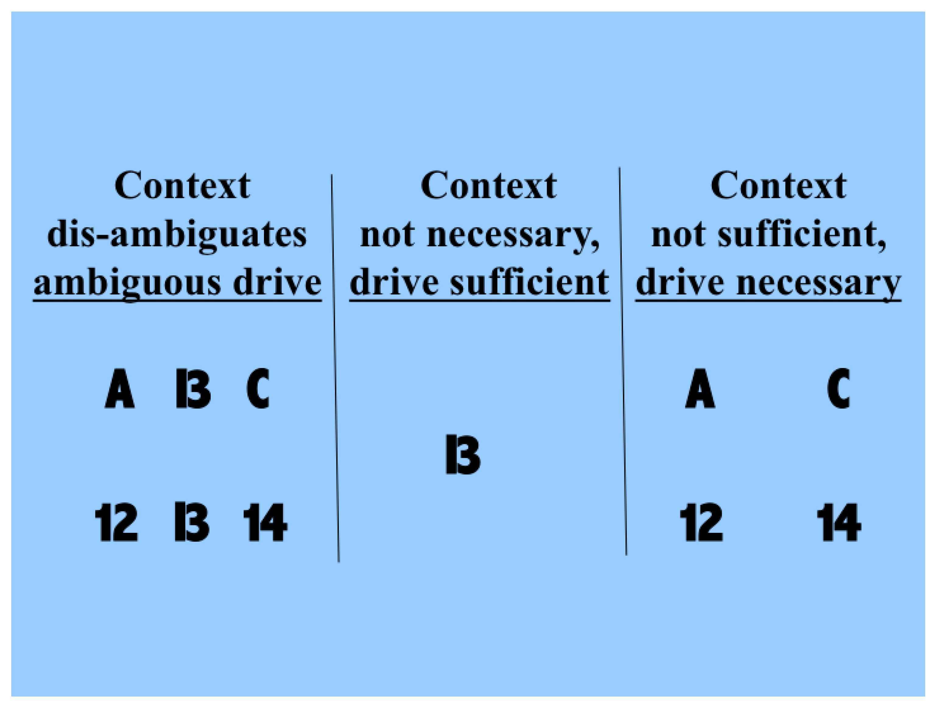A simple example of our notion of contextual modulation is shown in Figure 1. The driving information with which we are concerned here is that provided by the symbol that can be seen as either a B or a 13. Each of these possible interpretations is at less than full strength because of the ambiguity. The two rows in the left column show that the probabilities of making each of the possible interpretations can be influenced by the context in which the ambiguous figure is seen. The central column shows that drive alone is sufficient for some input information to be transmitted, and that context is not necessary because in its absence we can still see that a symbol that could be a B or a 13 is present. The right column shows that drive is necessary and that context is not sufficient, because when the information that is disambiguating in the left column is present in the absence of the driving information we do not see the B or 13 as being present. Though simple, and but one of indefinitely many, this demonstration shows that human neocortex uses context to interpret input in a way that is essentially asymmetric.

Therefore, contextual modulation cannot be implemented by purely multiplicative interactions, as often implied. Multiplication may indeed be involved in a more complex expression describing contextual modulation, as indeed it is for forms of contextual modulation advocated here. The crucial asymmetry does not arise by virtue of that multiplication, however, but by virtue of other things, such as asymmetric limitations on the interacting terms, or by adding one term but not the other to the result of the multiplication.

Though the information used for disambiguation in the example of Figure 1 comes from nearby locations in space, contextual modulation is not identified with any particular location in space because modulatory signals can in principle come from anywhere, including other points in time as well as other locations in space. Furthermore, though the example given here is contrived to make the ambiguity to be resolved obvious to introspection, the ambiguities that we assume to be resolvable by context are more general, and include those due to weak signal to noise ratios, as well as those due to ambiguities of dynamic grouping and of task relevance. In short, we assume that contextual modulation uses other available information to amplify the transmission of ‘relevant’ signals without corrupting their semantic content, i.e., what they transmit information about. Here we use partial information decomposition to show how that is possible.

The information whose transmission is amplified or attenuated has been referred to as the ‘driving’ input, the ‘receptive field (RF)’ input, or the input that specifies the neuron’s ‘selective sensitivity’. Though none of these terms is wholly satisfactory, here we refer to the input about which information transmission is to be modulated as the driving receptive field (RF) input, and the modulatory input as the contextual field (CF) input.

One major contrast between hierarchies of abstraction in neocortex and those in deep learning systems is that intermediate levels of abstraction in neocortex typically have their own intrinsic utility, in addition to being on a path to even higher abstractions. There are outputs to subcortical sites from all levels of neocortical hierarchies, not only from a ‘top’ level. Furthermore, the functional and anatomical asymmetries that we emphasize are most clear for the class of pyramidal cells that provide those outputs from neocortex. Another major contrast is that contextual modulation in neocortex is provided by lateral and feedback connections, and it guides the current processing of all inputs; whereas in nets trained by deep learning back-propagation from higher levels is used only for training the system how to respond to later inputs. The work reported here contrasts with the simplifying assumption that neural systems are composed of leaky integrate-and-fire point neurons. Instead we emphasize functional capabilities that can arise in a local processor, or neuron, with two distinct sites of processing, i.e., two-point processors, as shown by partial information decomposition [29,32]. An anatomical asymmetry that may be associated with this functional asymmetry is obvious and long known. Pyramidal cells in mammalian neocortex have two distinct dendritic trees. One, the basal tree, feeds directly into the soma, from where the output signals are generated. The other is the apical dendritic tree, or tuft, which is much further from the soma and connected to it via the apical trunk. Inputs to these two trees come from very different sources, with the basal tree receiving the narrowly specified inputs about which the cell transmits information, while the apical tree receives information from a much broader context. Wide-ranging, but informal, reviews of evidence on this division of labor between driving and modulatory inputs within neocortical pyramidal cells indicate that it has fundamental implications for consciousness and cognition [13,34]

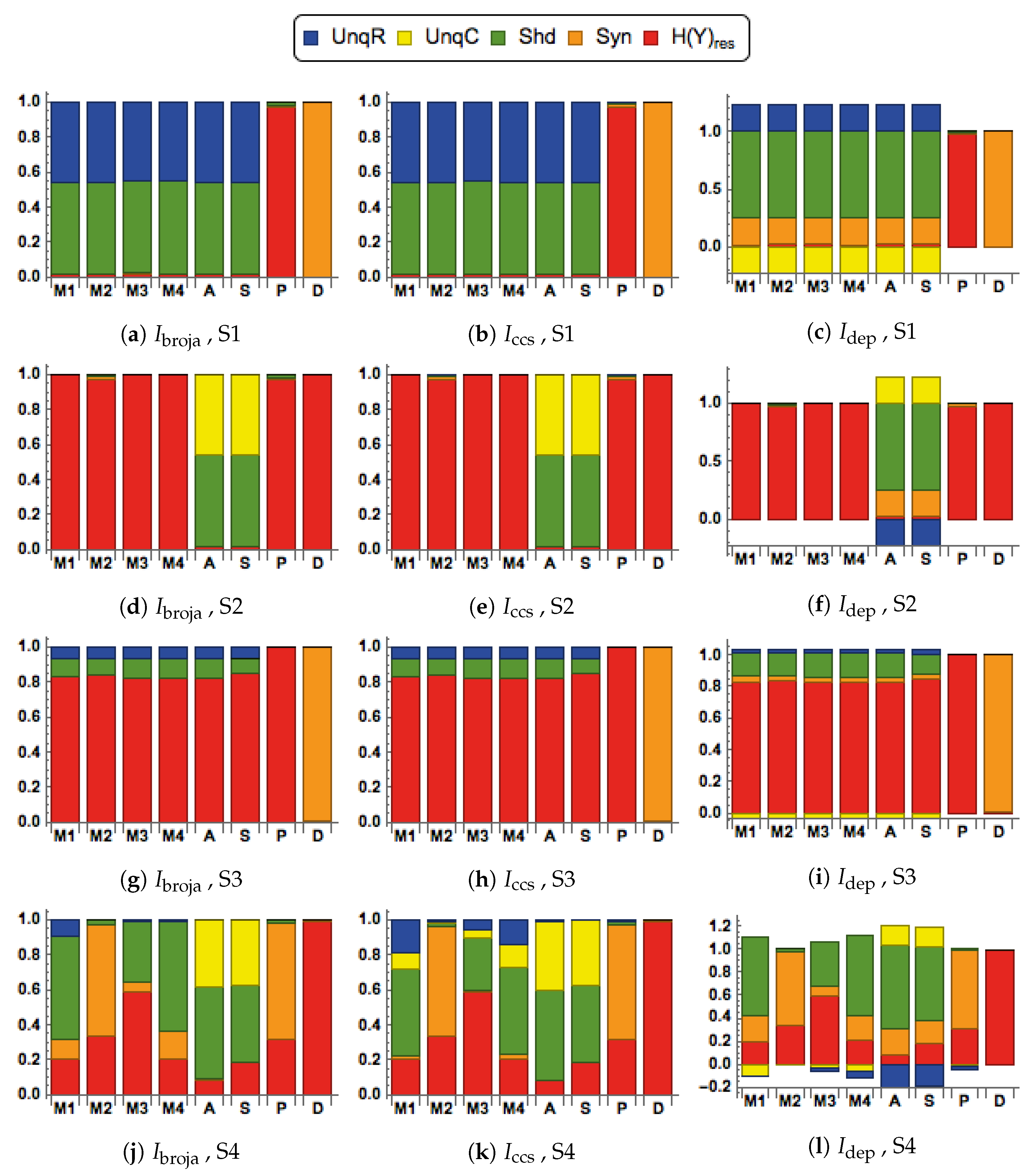
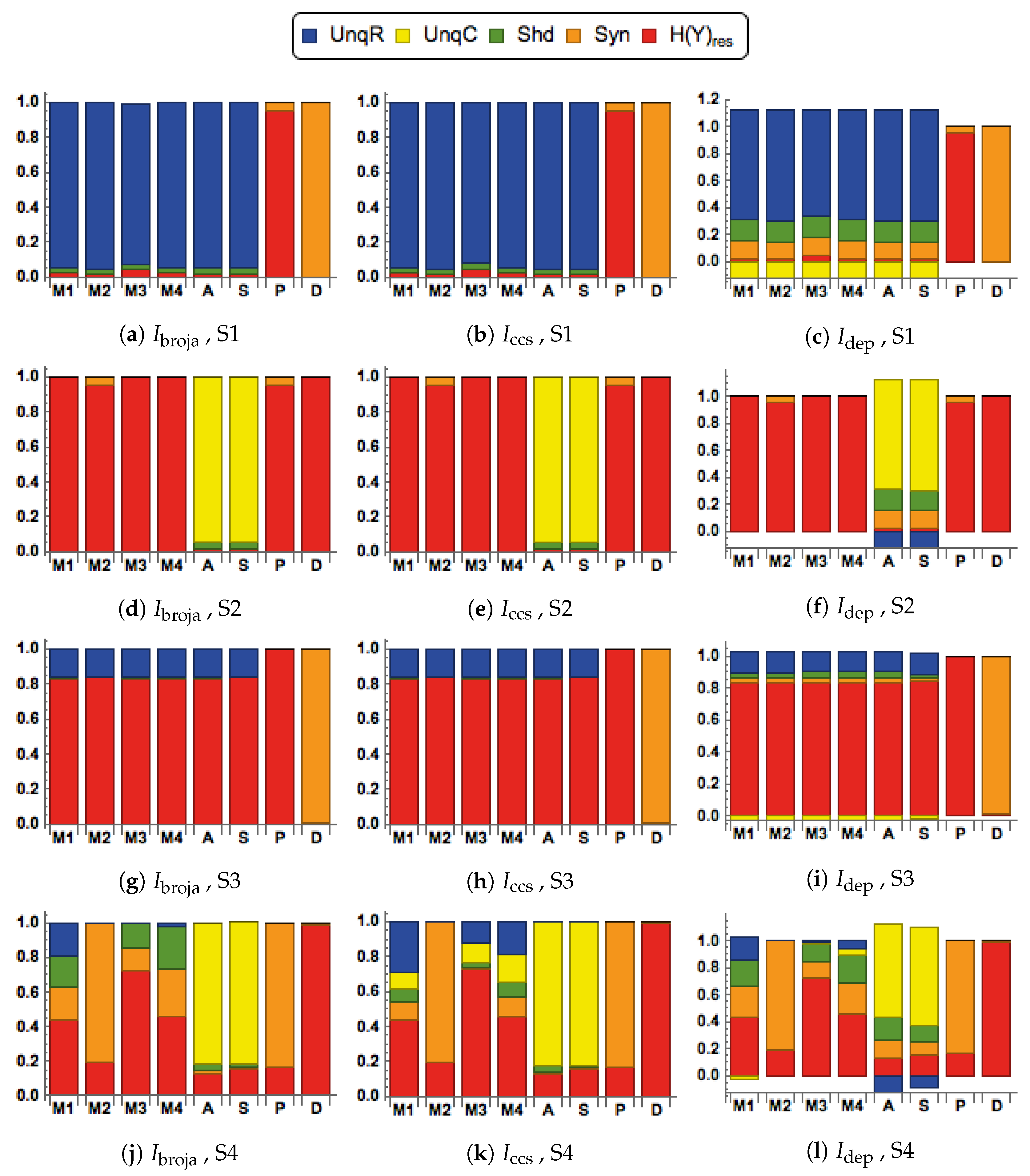
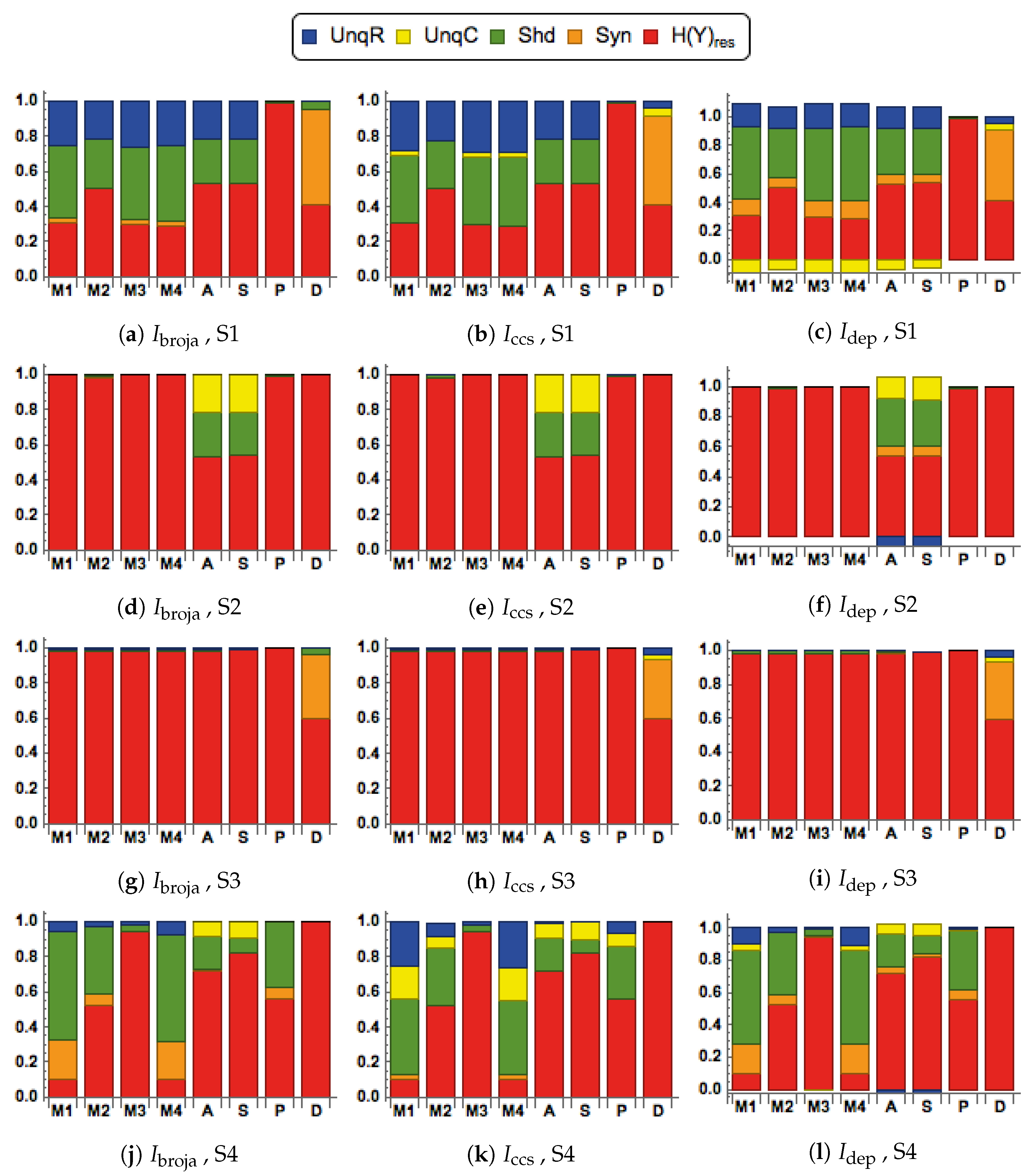
To further study these issues rigorously we use multivariate mutual information decomposition [28] to analyze the information transmitted by one binary output variable, e.g., an output action potential or brief burst of action potentials, given two input variables, and we consider five different types of partial information decomposition. The partial information decompositions of four different forms of contextual modulation are studied. Those decompositions are compared with decompositions of purely additive, subtractive, multiplicative, or divisive transfer functions. Here we consider continuous inputs that are generated from multimodal and unimodal Gaussian probability models. The eight different forms of interaction are considered for each of four scenarios in which the signal strengths given to the two inputs are different. These strength scenarios are chosen to show the distinctive information processing properties of contextual modulation. These properties are as follows. First, information uniquely about the drive can be transmitted when contextual modulation is absent or very weak, and all of it is transmitted if the drive is strong enough. Second, little or no information or misinformation is transmitted uniquely about the modulatory input when drive is absent or very weak whatever the strength of the modulation. Third, modulatory inputs can amplify or attenuate the transmission of driving information that is weak or ambiguous. We show that this modulation is characterized by a synergistic component of the output that is present at intermediate levels of drive strength, but not at either very high or very low levels. Finally, we provide evidence that contextual modulation is asymmetric at the cellular level in neocortex by applying partial information decomposition to a highly detailed multi-compartmental model of a layer 5 pyramidal cell and showing that it functions in a way that approximates contextual modulation as defined above.

The work reported here builds on some long-established principles of cognition and neuroscience, but also offers a clear advance beyond them. Our conception of contextual modulation builds upon the view, long held by philosophers such as Immanuel Kant, that basic perception and other cognitive functions are in effect ‘unconscious inference’ [35]. There is now ample evidence from psychophysics to neurophysiology to support and extend that view [12,36]. Though proposed by us more than 25 years ago, the conception of local processors as having two points of integration is not yet widely shared by those who work on systems neuroscience, many of whom remain fully committed to the assumption that, from the functional point of view, neurons in general can be adequately conceived of as leaky integrate-and-fire point neurons [37]. That is beginning to change, however, because evidence from intracellular recordings at well-separated points on a single neuron is now becoming too strong to ignore [9,13]. Partial information decomposition is a very recent extension to the foundations of information theory. It has great potential for use in the cognitive and neurosciences, as well as in artificial intelligence and neuromorphic computing. Its application to such issues has just begun [28], but it has far to go. Use of two-point processors in artificial neural nets is also beginning [38], but not yet in the form of the context-sensitive two-point processors analyzed here. When context-sensitive two-point processors are used in such applications new light may be cast on well-established difficulties in the use of context, such as getting stuck in ‘local minima’ within the contextual landscape, and interference between competing contexts. This is the first paper in which partial information decomposition is used to explicitly distinguish the information processing properties of context-sensitive two-point processors from those of the simple arithmetic operators.

2. Methods

2.1. Notation and Definitions

A nomenclature of mathematical terms and acronyms is provided at the end of the paper.

In [29], a local processor with two binary inputs and a binary output was discussed. Here, the inputs are instead continuous and have an absolutely continuous probability density function (p.d.f.), defined on ${\mathbb{R}}^2$. We denote the inputs to the processor by the continuous random variables R and C (where R stands for the receptive field drive and C for the contextual input), and the output by the binary random variable, Y, taking values in the set $\{-1,1\}$. The conditional distribution of Y, given that $R=r,C=c$ is Bernoulli with conditional probability of the logistic form

$$Pr(Y=1|R=r,C=c)=1/(1+exp(-T(r,c\left)\right),$$

(1)

where $T(r,c)$ is a continuous function defined on ${\mathbb{R}}^2$.

We now define the standard information-theoretic terms that are required in this work and based on results in [39,40]. We denote by the function H the usual Shannon entropy, and note that any term with zero probabilities makes no contribution to the sums involved. The joint mutual information that is shared by Y and the pair $(R,C)$ is given by,

$$I(Y;R,C)=H\left(Y\right)+H(R,C)-H(Y,R,C).$$

(2)

The information that is shared between Y and R but not with C is

$$I(Y;R|C)=H(Y,C)+H(R,C)-H(C)-H(Y,R,C),$$

(3)

and the information that is shared between Y and C but not with R is

$$I(Y;C|R)=H(Y,R)+H(R,C)-H(R)-H(Y,R,C).$$

(4)

The information shared between Y and R is

$$I(Y;R)=H\left(Y\right)+H\left(R\right)-H(Y,R)$$

(5)

and between Y and C is

$$I(Y;C)=H\left(Y\right)+H\left(C\right)-H(Y,C)$$

(6)

The interaction information [41] is a measure of information involving all three variables, $Y,R,C$ and is defined by

$$II(Y;R;C)=I(Y;R,C)-I(Y;R)-I(Y;C)$$

(7)

It has been employed as a measure of synergy [42,43].

2.2. Partial Information Decompositions

Partial Information Decomposition (PID) was introduced by Williams and Beer [30]. It provides a framework under which the mutual information, shared between the inputs and the output of a system, can be decomposed into components which measure four different aspects of the information: the unique information that each input conveys about the output; the shared information that both inputs possess regarding the output; the information that the inputs in combination have about the output. Partial information decomposition has been applied to data in neuroscience; see, e.g., [31,44,45,46]. For a recent overview, see [28]. The PIDs were computed using the freely available Python package, dit [47].

Here there are two inputs, $R,C$, and one output, Y. The information decomposition can be expressed as [32]

$$I(Y;R,C)=I_{unq}(Y;R|C)+I_{unq}(Y;C|R)+I_{shd}(Y;R,C)+I_{syn}(Y;R,C).$$

(8)

Adapting the notation of [32] we express our joint input mutual information in four terms as follows:

It is possible to make deductions about a PID by using the following four equations which give a link between the components of a PID and certain classical Shannon measures of mutual information. The following are in (Equations (4) and (5), [32]), with amended notation; see also [30].

$$\begin{array}{cc}\hfill I(Y;R)& =\mathrm{Unq}R+\mathrm{Shd}\hfill \end{array}$$

(9)

$$\begin{array}{cc}\hfill I(Y;C)& =\mathrm{Unq}C+\mathrm{Shd},\hfill \end{array}$$

(10)

$$\begin{array}{cc}\hfill I(Y;R|C)& =\mathrm{Unq}R+\mathrm{Syn},\hfill \end{array}$$

(11)

$$\begin{array}{cc}\hfill I(Y;C|R)& =\mathrm{Unq}C+\mathrm{Syn}.\hfill \end{array}$$

(12)

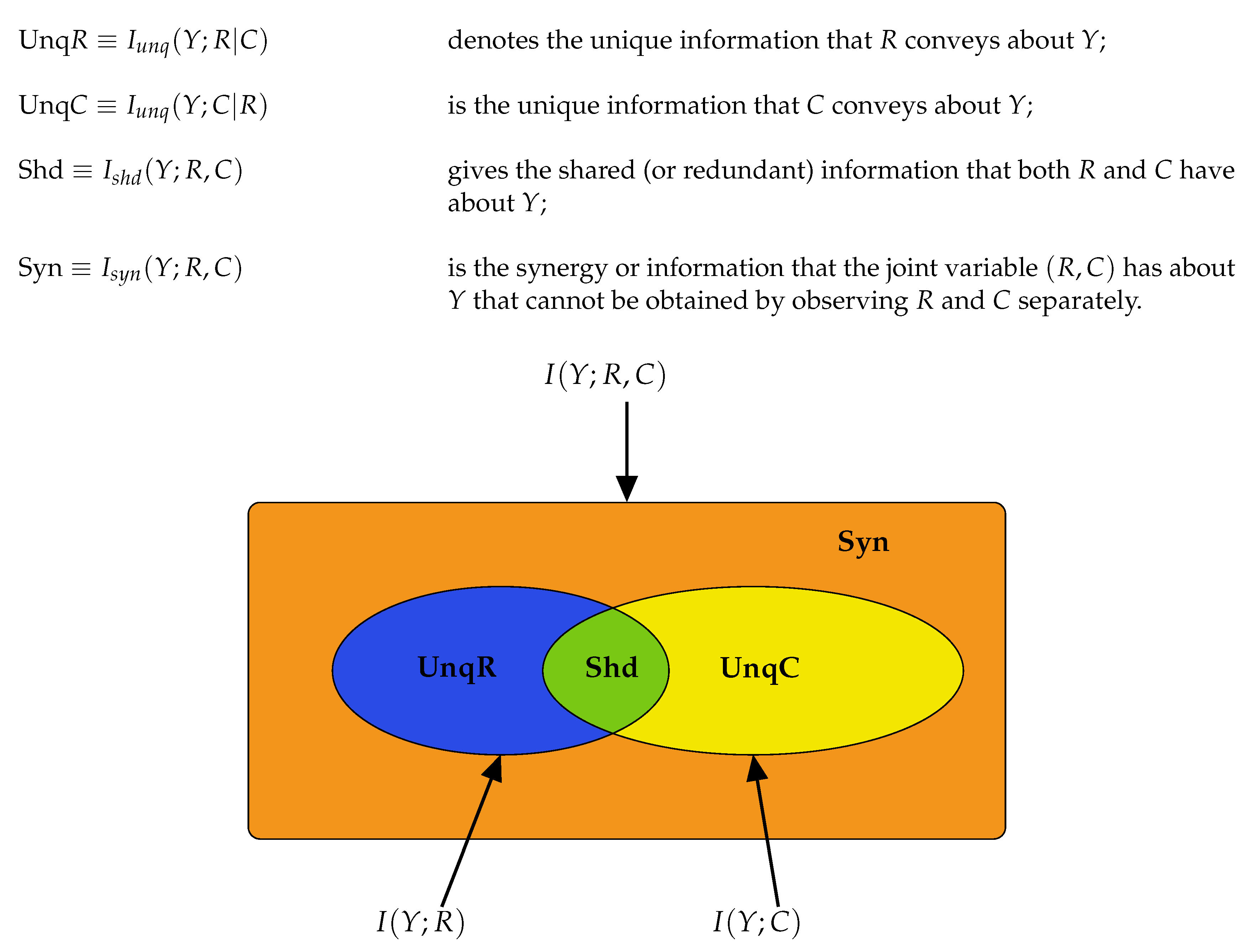
The Equations (8)–(10) are illustrated in graphical format in Figure 2. Using (8)–(10) we may deduce the following connections between classical information measures and partial information components.

$$II(Y;R;C)=\mathrm{Syn}-\mathrm{Shd}$$

(13)

$$I(Y;R)-I(Y;C)=\mathrm{UnqR}-\mathrm{UnqC}$$

(14)

When the partial information components are all non-negative, we may deduce the following from $\left(2\right)$, $\left(9\right)$ and $\left(10\right)$. When the interaction information in $\left(7\right)$ is positive, a lower bound on the synergy of a system is given by the interaction information [41]. Also, the expression in $\left(14\right)$ provides a lower bound for UnqR, when $I(Y;R)>I(Y;C)$. Thus, some deductions can be made without considering a PID. While such deductions can be useful in providing information bounds, it is only by computing a PID that the actual values of the partial information components can be obtained.

We consider here five of the different information decompositions that have been proposed. The five methods of decomposition are $I_{\min }$ [30], $I_{\mathrm{proj}}$ [48], $I_{\mathrm{broja}}$ [49,50], $I_{\mathrm{ccs}}$ [51] and $I_{\mathrm{dep}}$ [52]. Although there are clear conceptual differences between them, our emphasis is upon aspects of the decompositions on which we find that they all agree.

In particular, all the PID methods, except $I_{\mathrm{ccs}}$, produce PID components that are non-negative, whereas $I_{\mathrm{ccs}}$ can produce negative values. The PID $I_{\mathrm{ccs}}$ is a pointwise-based method in which local information measures are employed at the level of individual realizations. This is also the case with fully pointwise PIDs, such as [53,54]. Local mutual information is explained by Lizier in [55]. If $U,V$ are discrete random variables then the mutual information $I(U,V)$ shared between U and V can be written as an average of the local mutual information terms $i(u;v)$, for each individual realization $(u,v)$ of $(U,V)$, as follows

$$I(U;V)=\sum _{u,v}p(u,v){log}_2\frac{p(u,v)}{p\left(u\right)p\left(v\right)}=\sum _{u,v}p(u,v){log}_2\frac{p\left(u\right|v)}{p\left(u\right)}=\sum _{u,v}p(u,v){log}_{2}i(u;v),$$

(15)

where

$$i(u;v)={log}_2\frac{p\left(u\right|v)}{p\left(u\right)}$$

is the local mutual information associated with the realization $(u,v)$ of $(U,V)$.

The local mutual information $i(u;v)$ is positive when $p\left(u\right|v)>p(u)$, so that “knowing the value of v increased our expectation of (or positively informed us about) the value of the measurement u” [55]. The local mutual information $i(u;v)$ is negative when $p\left(u\right|v)<p(u)$, so that “knowing about the value of v actually changed our belief $p\left(u\right)$ about the probability of occurrence of the outcome u to a smaller value $p\left(u\right|v)$, and hence we considered it less likely that u would occur when knowing v than when not knowing v, in a case were u nevertheless occurred” [55]. Of course, the average of these local measures is the mutual information $I(U;V)$, as in $\left(15\right)$, but when pointwise information measures are used to construct a PID there can be negative averages. For further details of how negative values of PID components can occur, see [53,54].

In the simulations, it will be found in some cases that the $I_{\mathrm{ccs}}$ PID has a negative value for the unique information due to context, C. We interpret this to mean that the unique information provided by C is, on average, less likely to result in predicting the correct value of the output Y. We adopt the term ‘misinformation’ from [53,54], and describe this as ‘unique misinformation due to context, C’.

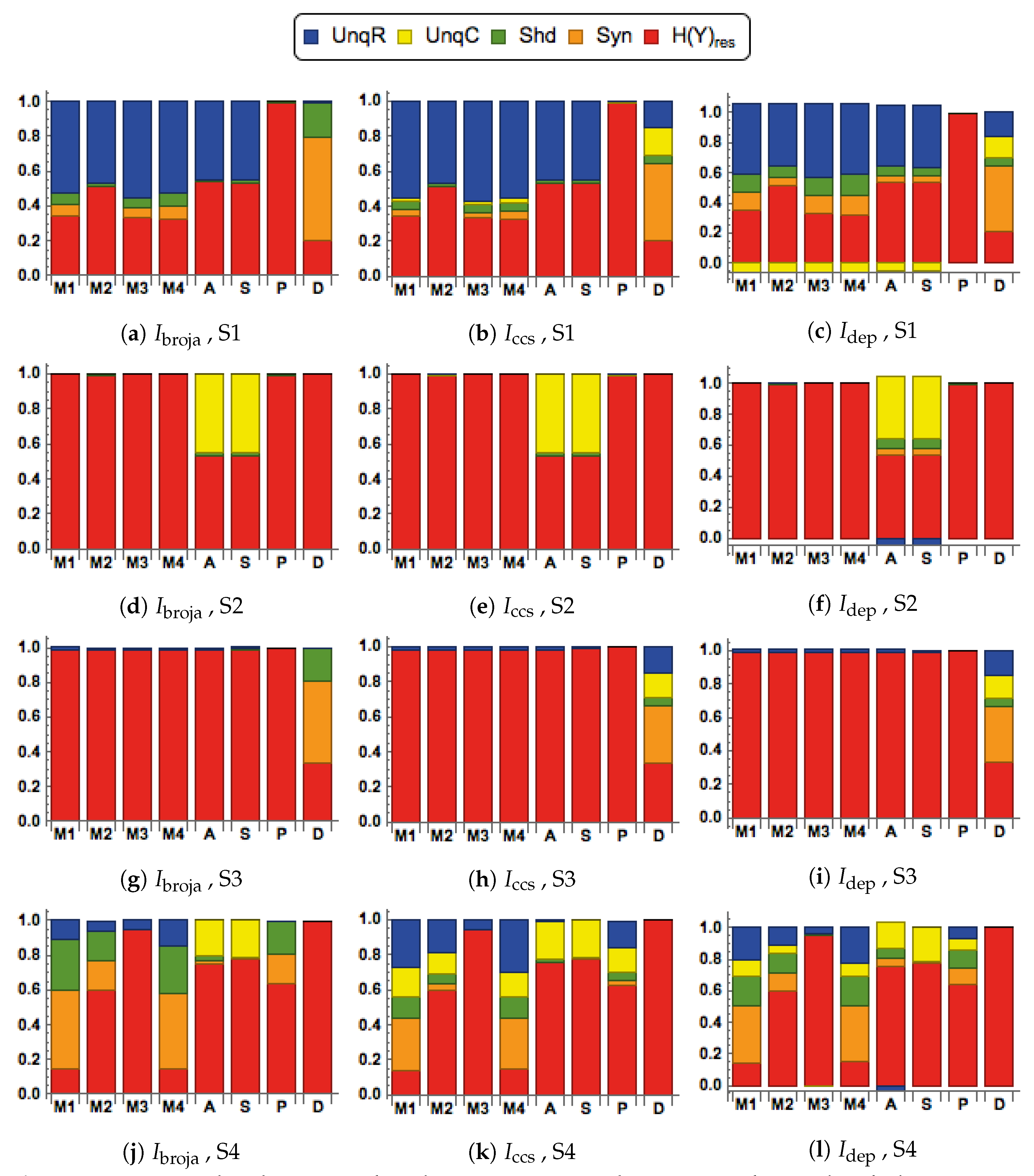
We also consider residual output entropy defined by $H{\left(Y\right)}_{\mathrm{res}}=H\left(Y\right|R,C)$. In addition to the four PID components, this residual measure is useful in expressing the information that is in Y but not in $R,C$. It is also worth noting that these five terms add up to the output entropy $H\left(Y\right)$, and when plotted we refer to the decomposition as a spectrum.

$$H\left(Y\right)=\mathrm{UnqR}+\mathrm{UnqC}+\mathrm{Shd}+\mathrm{Syn}+H{\left(Y\right)}_{\mathrm{res}}.$$

(16)

When making comparisons between different systems it is sometimes necessary to normalize the five measures in $\left(16\right)$ by dividing each term by their total, the output entropy, $H\left(Y\right)$. Such normalization was applied in some systems that are considered in Section 3.1.

2.3. Transfer Functions

We consider eight different forms of transfer function when computing the conditional output probabilities in $\left(1\right)$. These transfer functions provide different ways of combining the two inputs. The functions in $\left(17\right)$ define modulatory forms of interaction, whereas those in $\left(18\right)$ are arithmetic. One aim of this study is to compare the PIDs obtained when using the different functions.

There are four modulatory transfer functions that are defined as follows.

$$\begin{array}{cc}\hfill T_{\mathrm{M}1}(r,c)& =\frac{1}{2}r(1+exp\left(rc\right))\hfill \\ \hfill T_{\mathrm{M}2}(r,c)& =r+rc\hfill \\ \hfill T_{\mathrm{M}3}(r,c)& =r(1+tanh\left(rc\right))\hfill \\ \hfill T_{\mathrm{M}4}(r,c)& =r{2}^{rc}\hfill \end{array}$$

(17)

We also consider four transfer functions that correspond to arithmetic interactions between the inputs. They are given by

$$T_{\mathrm{A}}(r,c)=r+c,T_{\mathrm{S}}(r,c)=r-c,T_{\mathrm{P}}(r,c)=rc,T_{\mathrm{D}}(r,c)=r/c.$$

(18)

2.4. Different Signal-Strength Scenarios

The inputs to the processor, $R,C$ are composed as $R=s_1{X}_1$ and $C=s_2{X}_2$, where $X_1,X_2$ are continuous random variables that have mean values of $\pm 1$. Then the mean values of R are $\pm s_1$ and the mean values of C are $\pm s_2$. The signal strengths, $s_1,s_2$, are non-negative real parameters that characterize the strength of each input.

Four combinations of signal strengths are used in this study, as defined in

Table 1. The four signal-strength scenarios

S1	Scenario 1: Strong R, with C near 0	($s_1=10.0,s_2=0.05$)
S2	Scenario 2: R near zero, with strong C	($s_1=0.05,s_2=10.0$)
S3	Scenario 3: Weak R, with C near 0	($s_1=1.00,s_2=0.05$)
S4	Scenario 4: Weak R, with moderate C	($s_1=1.00,s_2=5.00$)

.

They are chosen to test for the key properties of contextual modulation. They are:

CM1:

The drive, R, is sufficient for the output to transmit information about the input, so context, C, is not necessary.

CM2:

The drive, R, is necessary for the output to transmit information about the input, so context, C, is not sufficient.

CM3:

The output can transmit unique information about the drive, R, but little or no unique information or misinformation about the context, C.

CM4:

The context can strengthen the transmission of information about R when R is weak.

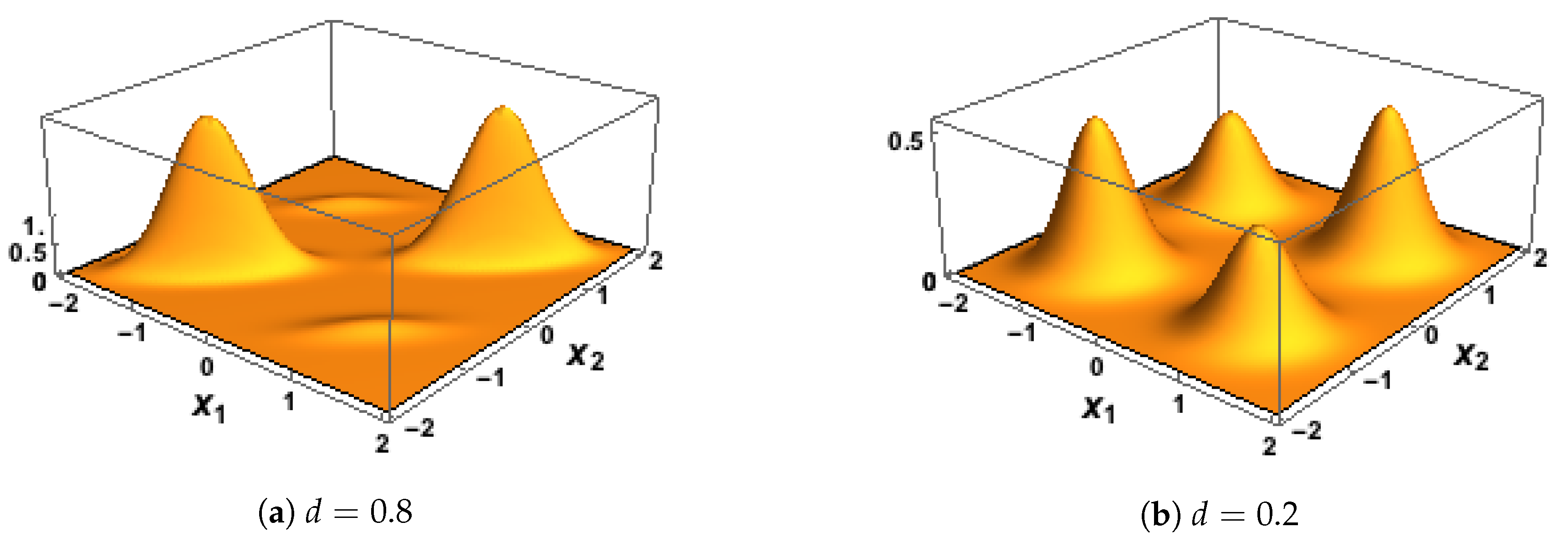
2.5. Bivariate Gaussian Mixture Model (BGM)

In earlier work [29], we considered units that are bipolar. The bivariate Gaussian mixture model offers a generalization to continuous inputs which reflect underlying binary events. We also consider a single bivariate Gaussian model for the inputs that is obviously more relevant to interactions between the two sites of integration within pyramidal cells. It is useful to know that two such different models for the inputs give essentially the same results on all the issues explored herein. We require the marginal distributions for the integrated receptive and contextual fields R and C to be bimodal, with the distribution of R with modes at $\pm s_1$ and the distribution of C with modes at $\pm s_2$. We shall define a bivariate Gaussian mixture model for $(R,C)$ which has four modes – at $(-s_1,-s_2),(-s_1,s_2),(s_1,-s_2)$ and $(s_1,s_2)$. First we consider the bivariate Gaussian mixture model for $(X_1,X_2)$, with probability density function

$$f(x_1,x_2|{\mu }_1,{\mu }_2,{\mu }_3,{\mu }_4,\mathsf{\Sigma })=\sum _{i=1}^4{\pi }_i{f}_i(x_1,x_2|{\mu }_i,\mathsf{\Sigma }),$$

(19)

where

$${\mu }_1=\left[\begin{array}{c}-1\\ -1\end{array}\right],{\mu }_2=\left[\begin{array}{c}-1\\ 1\end{array}\right],{\mu }_3=\left[\begin{array}{c}1\\ -1\end{array}\right],{\mu }_4=\left[\begin{array}{c}1\\ 1\end{array}\right],\mathsf{\Sigma }={\sigma }^2\left[\begin{array}{cc}1& \rho \\ \rho & 1\end{array}\right]$$

and the $\left\{{\pi }_i\right\}$ are the mixing proportions that are non-negative and sum to unity. For simplicity, we have assumed that the bivariate Gaussian pdfs, which form the four components of the mixture, have the same covariance matrix and also that the variances of $X_1$ and $X_2$ are equal. We note, in particular, that the correlation between $X_1$ and $X_2$ is equal to $\rho$ in all four of the component distributions.

However, we require investigation of, the correlation of $X_1$ and $X_2$ for the mixture distribution defined by $f(x_1,x_2|{\mu }_1,{\mu }_2,{\mu }_3,{\mu }_4,\mathsf{\Sigma })$ and, in particular, we need to find a way of setting this correlation to take any desired value in the simulations. We proceed as follows.

Consider the random vector X given by

$$X=\left[\begin{array}{c}{X}_1\\ X_2\end{array}\right]$$

Then, with respect to the mixture model $\left(19\right)$, X has mean vector

$$\mathbb{E}\left(X\right)=\sum _{i=1}^4{\pi }_i\mathbb{E}\left(X\right|i)=\sum _{i=1}^4{\pi }_i{\mu }_i=\left[\begin{array}{c}-{\pi }_1-{\pi }_2+{\pi }_3+{\pi }_4\\ -{\pi }_1+{\pi }_2-{\pi }_3+{\pi }_4\end{array}\right],$$

where we have used the law of iterated expectation. We make the simplifying assumption that ${\pi }_4={\pi }_1$ and that ${\pi }_3={\pi }_2$ which results in both components of $\mathbb{E}\left(X\right)$ being equal to zero. This assumption also means that ${\pi }_1+{\pi }_2=\frac{1}{2}.$

We denote the covariance matrix of X in the mixture model $\left(19\right)$ by K. Then

$$K=\mathbb{E}\left[(X-\mu ){(X-\mu )}^T\right]=\mathbb{E}\left(X{X}^T\right)-\mu {\mu }^T=\mathbb{E}\left(X{X}^T\right),$$

since $\mu$ is the zero vector. Now, again using the law of iterated expectation, we have that

$$\mathbb{E}\left(X{X}^T\right)=\sum _{i=1}^4{\pi }_i\mathbb{E}\left(X{X}^T\right|i)=\sum _{i=1}^4{\pi }_i(\mathsf{\Sigma }+{\mu }_i{\mu }_i^T)=\mathsf{\Sigma }+\sum _{i=1}^4{\pi }_i{\mu }_i{\mu }_i^T,$$

which simplifies to

$$K=\mathbb{E}\left(X{X}^T\right)=\left[\begin{array}{cc}{\sigma }^2+1& \rho {\sigma }^2+2{\pi }_1-2{\pi }_2\\ \rho {\sigma }^2+2{\pi }_1-2{\pi }_2& {\sigma }^2+1\end{array}\right].$$

Therefore, in the mixture model $\left(19\right)$, the Pearson correlation coefficient of $X_1$ and $X_2$ is

$$\mathrm{cor}(X_1,X_2)=\frac{\rho {\sigma }^2+2{\pi }_1-2{\pi }_2}{{\sigma }^2+1}.$$

Setting this expression to be equal to the desired value of the correlation, d, gives that

$${\pi }_1-{\pi }_2=\frac{1}{2}(d-(\rho -d){\sigma }^2).$$

Taking $\rho =d$ and using the equality ${\pi }_1+{\pi }_2=\frac{1}{2}$ gives that

$${\pi }_1=(1+d)/4\equiv \lambda \mathrm{and}{\pi }_2=(1-d)/4\equiv \mu .$$

Hence, to generate values of $(X_1,X_2)$ from the BGM model that have correlation d we take

$$\mathsf{\Sigma }={\sigma }^2\left[\begin{array}{cc}1& d\\ d& 1\end{array}\right],{\pi }_4={\pi }_1=\lambda \mathrm{and}{\pi }_3={\pi }_2=\mu ,$$

for some pre-selected value of $\sigma$.

Now let $R=s_1{X}_1$ and $C=s_2{X}_2$. Then $(R,C)$ has the same correlation as $(X_1,X_2),$ by the invariance of Pearson correlation under linear transformation, and it has a bivariate Gaussian mixture model with component means

$$\left[\begin{array}{c}-s_1\\ -s_2\end{array}\right],\left[\begin{array}{c}-s_1\\ s_2\end{array}\right],\left[\begin{array}{c}{s}_1\\ -s_2\end{array}\right],\left[\begin{array}{c}{s}_1\\ s_2\end{array}\right]$$

and component covariance matrices all equal to

$${\sigma }^2\left[\begin{array}{cc}{s}_1^2& d{s}_1{s}_2\\ d{s}_1{s}_2& s_2^2\end{array}\right],$$

with mixing proportions $\{\lambda ,\mu ,\mu ,\lambda \}$. It follows from the above discussion that in the bivariate Gaussian mixture model $\left(19\right),$ $(R,C)$ has mean vector $\mu$ and covariance matrix K given by

$$\mu =\left[\begin{array}{c}0\\ 0\end{array}\right]\mathrm{and}K=({\sigma }^2+1)\left[\begin{array}{cc}1& d\\ d& 1\end{array}\right].$$

Some plots of the BGM probability density function are given in Figure 3. To complete the 3D specification of the joint distribution for $(Y,R,C)$ the conditional distribution of Y, given that $R=r$ and $C=c$, was assumed to be Bernoulli with probability equal to the logistic function applied to $T(r,c)$, as in $\left(1\right)$.

2.6. Single Bivariate Gaussian Model (SBG)

While in our previous work [29] bipolar inputs have been considered, and a continuous version considered in Section 2.5, there are many datasets in neuroscience and in machine learning where the input variables are not bimodal. We extend our approach, therefore, by considering the input data to have been generated from a single bivariate Gaussian probability model. We take $(X_1,X_2)$ to have a bivariate Gaussian distribution, with mean vector and covariance matrix

$$\mu =\left[\begin{array}{c}1\\ 1\end{array}\right],\mathsf{\Sigma }={\sigma }^2\left[\begin{array}{cc}1& d\\ d& 1\end{array}\right].$$

Then, R and C are bivariate Gaussian, with mean vector and covariance matrix

$$\mu =\left[\begin{array}{c}{s}_1\\ s_2\end{array}\right],\mathsf{\Sigma }={\sigma }^2\left[\begin{array}{cc}{s}_1^2& d{s}_1{s}_2\\ d{s}_1{s}_2& s_2^2\end{array}\right].$$

Taking $\sigma =0.3$, ensures that almost 100% of the generated values of $(X_1,X_2)$ lie within the unit square $[0,2]\times [0,2]$, and so the corresponding values of R and C are almost certainly positive.

Given positive inputs, it is necessary to introduce a bias term, b, into each transfer function. Thus, the general $T(r,c)$ is replaced here by

$$T_b(r,c)=T(r,c)-b,$$

where b is taken to be the median of the values of $T(r,c)$ obtained by plugging in the generated values of r and c. This choice of b ensures that the simulated outputs are equally likely to be $+1$ or $-1$, so the output entropy $H\left(Y\right)$ will be very close to its maximum value of 1. The conditional output probabilities are computed using $\left(1\right)$, with $T(r,c)$ replaced by $T_b(r,c)$ for each of the transfer functions in (17) and (18).

2.7. First Simulation, with Inputs Generated Using the BGM Model

The first simulation study has four factors: transfer function, PID method, scenario and the correlation between the inputs. For each combination of the eight transfer functions, four signal-strength scenarios and two values of correlation (0.8, 0.2), data were generated using the following procedure.

One million samples of $(X_1,X_2)$ were generated from the bivariate Gaussian mixture model in $\left(19\right)$ for a given value of the correlation, d, a given combination of the signal strengths, $s_1,s_2$ and a given transfer function. In all cases the standard deviation of $X_1$ and $X_2$ was taken as $\sigma =0.3$.

For each sample, the values of R and C were computed as $r=s_1{x}_1$ and $c=s_2{x}_2$, and these values were passed through the appropriate transfer function to compute the conditional output probability, ${\theta }_{rc}$ in $\left(1\right)$. For each value of $r,c$ a value of Y was simulated from the Bernoulli distribution with probability, ${\theta }_{rc}$, thus giving a simulated data set for $(Y,R,C)$.

Given the that PIDs have not yet been developed for this type of data, it is necessary to bin the data. For each data set, a hierarchical binning procedure was employed. The values of R were separated according to sign, and then the positive values were split equally into three bins using tertiles, and similarly for the negative values of R. The same procedure was used to define bins for the values of C.

The values of the binary output Y were binned according to sign. Having defined the bins, the one million $(Y,R,C)$ observations were allocated to the appropriate bins. This procedure produced a $6\times 6\times 2$ probability array that was used in each case as input for the computation of each of the five PIDs used in the study, making use of the package, dit, which is available on GitHub (https://github.com/dit/dit).

2.8. The Second Simulation, with Inputs Generated Using the SBG Model

The second simulation study is essentially a repeat of the first study, as described in Section 2.6, with the continuous input data for R and C being generated using the SBG model of Section 2.6 rather than the BGM model. The values of the binary output Y were simulated in a similar way, with transfer functions of the form $T_b(r,c)$ used rather than $T(r,c)$. The binning of the data was performed in a slightly different way. Given the absence of bipolarity here, the values of R were divided equally into six bins defined by sextiles, and similarly for C. The binary outputs were split according to sign. Thus, again here, a $6\times 6\times 2$ probability array was created, and it was used in each case to compute the PIDs.

3. The Results

The PIDs obtained using the methods, $I_{\min }$, $I_{\mathrm{proj}}$, $I_{\mathrm{broja}}$, were almost identical in both simulations, so we show results only for the $I_{\mathrm{broja}}$ method. Thus, anything said in the ensuing about this method also applies to the $I_{\min }$ and $I_{\mathrm{proj}}$ PIDs.

3.1. First Simulation, with Inputs Generated Using the BGM Model

Here, each input is generated from a bimodal Gaussian distribution which has four modes, as defined near $\left(19\right)$. The results are presented in Figure 4 and Figure 5 in a way that makes it easy to make many different comparisons if the color scheme for depicting the five different components is learned. They show that different transfer functions can transmit similar components of input information in some signal-strength scenarios, but very different components under other scenarios. The rich variety of spectra produced provides a new perspective on the information processing capabilities of each of the transfer functions. In particular, they show that the components of information transmitted by contextual modulation differ greatly from those of all four simple arithmetic operators, including multiplication and division, which are also often thought of as modulatory.

The asymmetrical effects of R and C on output when using a modulatory transfer are clear. The first row of spectra in Figure 4 is for strong drive and weak modulation. Nearly all the input information is transmitted, half as that unique to the drive, shown in blue, and half as a shared component due to the correlation between the two inputs. The second row of spectra is for the reverse strength scenario. In that case no information is transmitted. The two bottom rows show that although modulatory transfer functions do not transmit information unique to the modulator (C), they do use that information to modulate output in cases where drive is present but weak.

3.1.1. Distinctive Information Transmission Properties of Contextual Modulation

The distinctive properties of contextual modulation can be seen by comparing the $I_{\mathrm{broja}}$ decomposition of M1, i.e., the left-most spectra in column 1 of Figure 4, with those of all four simple arithmetic operators. The four rows show these decompositions for each of the four different signal-strength scenarios. M1 transmits the same or very similar components as additive and subtractive operators when context strength is close to zero. Thus, in the absence of contextual information, it defaults to near-equivalence with the additive and subtractive operators. The effects of contextual modulation differ greatly from those of addition and subtraction when drive strength approaches zero, however. In that case no input information is transmitted by the modulatory interaction whereas additive and subtractive operators transmit all or most of the input information in the form of the shared component and that unique to the stronger input. These comparisons show that drive is both necessary and sufficient for transmission of input information by the contextual modulatory interaction, M1, and that contextual input is neither necessary nor sufficient. Thus, this clearly displays the marked asymmetry between the effects of driving and modulatory input that is a distinctive property of contextual modulation.

In Figure 5, the correlation between R and C is weak (0.2), rather than strong (0.8), and this produces some clear differences in the expression of some information components when the spectra are compared with the corresponding spectra in Figure 4. For all transfer functions, except the multiplicative transfer function, P, and the divisive transfer function, D, there has been a large reduction in shared information, with a corresponding increase in the values of the unique information. This is not surprising since the part of the shared information that is due to the correlation between the inputs must decrease as the correlation between inputs is changed from strong to weak.

All of the conclusions regarding the comparisons of the modulatory with the arithmetic transfer functions that are discussed above, where the correlation between inputs is strong, apply here also when this correlation is weak, as do the conclusions regarding contextual modulation.

For both values of the correlation between the inputs we note the following. The components transmitted by M1 differ greatly from those of the multiplicative and divisive operators under all signal-strength scenarios. The multiplicative and divisive operators predominantly transmit synergistic components. They never transmit unique components. Contextual modulation does transmit some synergy, but that is much smaller than that transmitted by either multiplication or division, and occurs only when drive is weak. When drive is strong enough it transmits large components of both shared information and of that unique to the drive Though contextual modulation is neither necessary nor sufficient for information transmission, its modulatory effects can be clearly seen by comparing the components transmitted by M1 when drive is weak and context is moderate in Figure 4j and Figure 5j, with those transmitted when drive is weak and context is near zero in Figure 4g and Figure 5g. Moderate context increases the transmission of information about the drive by 0.4 bits. Stronger contextual inputs increase it even further. This increase is predominantly in the shared information but does include some increase in the component unique to the drive, and an increase in the synergistic component.

These fundamental contrasts between contextual modulation and the arithmetic operators apply also to the forms of interaction labeled as M2, M3, and M4, but with a few differences in some of the signal-strength scenarios. No differences between the four forms of contextual modulation occur when the strength of either the drive or the context is near zero. When neither is near zero the main effect of M2 is to greatly increase the synergistic component, resembling P. When drive is weak and context is strong M2 transmits mainly synergy, and is not at all effective in amplifying transmission of either the unique or shared information in the drive. M3 and M4 in that case do amplify transmission of shared information, but not of that unique to the drive. Over all scenarios only M1 uses context to increase the transmission of information unique to the drive.

3.1.2. Comparison of Five Different Forms of Information Decomposition

Encouraging convergence of the PID methodologies is indicated by our finding that the $I_{\mathrm{broja}}$ decomposition gives essentially the same results as $I_{\min }$ and $I_{\mathrm{proj}}$. Furthermore, the distinctive properties of contextual modulation seen when using the $I_{\mathrm{broja}}$ decomposition still apply when using the other forms, except for a few differences that are as follows. The PIDs $I_{\mathrm{dep}}$ and $I_{\mathrm{ccs}}$ differ from $I_{\mathrm{broja}}$, $I_{\min }$ and $I_{\mathrm{proj}}$, mainly in that when neither drive nor context are near zero they show that M1, M3 and M4 transmit some information unique to the context ($I_{\mathrm{dep}}$) and some misinformation unique to the context ($I_{\mathrm{ccs}}$), whereas $I_{\mathrm{broja}}$ does not. Therefore, the $I_{\mathrm{dep}}$ and $I_{\mathrm{ccs}}$ PIDs in Figure 4k do not support condition CM3 for contextual modulation.

In contrast to all the other methods the $I_{\mathrm{ccs}}$ PID can have negative unique information components. From $\left(9\right)$–$\left(12\right)$ it can be seen that a negative value for UnqR or UnqC corresponds the value of Shd or Syn or both being larger than they would be if the unique components were non-negative. Therefore, the $I_{\mathrm{ccs}}$ spectra can cover a range of approximately 1.4 instead of the range of 1 for the other PID methods. Nevertheless, in Scenario 1, the spectra for P and D are exactly the same as those obtained using $I_{\mathrm{broja}}$ and $I_{\mathrm{dep}}$. For the other transfer functions, which have almost identical spectra, the fact that UnqC is about −0.2 means that the synergy and shared components in these six spectra are correspondingly larger by 0.2. In Scenario 2, all the spectra are the same except for A and S. In this case, a negative value for UnqR leads to the presence of non-zero synergy and a larger estimate of the shared information. The spectra for Scenario 3 are almost the same as the corresponding transfer functions with $I_{\mathrm{broja}}$ and $I_{\mathrm{dep}}$, and so similar comments apply. In Scenario 4, the patterns of the spectra and the comparisons between them are essentially the same as those in the $I_{\mathrm{broja}}$ PIDs and so similar comparisons apply here, although the presence of negative unique components distorts the values of the other PID components, thus giving the spectra a somewhat different appearance.

In all four scenarios, transfer functions P and D have the same spectra for all five of the PID methods. For Scenarios 1–3, all five PID methods show the same results for each transfer function, with the exception of functions A and S in Scenario 2 (d, e, f) in which $I_{\mathrm{ccs}}$ has different spectra than those obtained with the other four methods. In Scenario 4, the spectra produced using $I_{\mathrm{dep}}$ are very similar to those obtained with $I_{\min }$, $I_{\mathrm{proj}}$ and $I_{\mathrm{broja}}$ except for the presence of larger values of UnqR and UnqC. Apart from functions P and D, the $I_{\mathrm{ccs}}$ spectra appear to be rather different from the corresponding spectra given with the other four methods due to the presence of negative values for UnqR and/or UnqC.

When the correlation between inputs is weak, as in Figure 5, all five PID methods produce the same spectra for P and D. For the remaining transfer functions, the corresponding $I_{\mathrm{broja}}$ and $I_{\mathrm{dep}}$ spectra are identical when either the drive or context is close to zero. When the drive is weak and the context is moderate, the corresponding $I_{\mathrm{dep}}$ and $I_{\mathrm{broja}}$ spectra are virtually identical for the arithmetic transfer functions, along with M2, whereas for M1, M2 and M3 $I_{\mathrm{dep}}$ produces larger unique components, and in particular positive values of information unique to the context.

When the correlation between inputs is weak, the negative components in $I_{\mathrm{ccs}}$ are smaller in magnitude. Apart from the negative unique components, the $I_{\mathrm{ccs}}$ spectra are very similar to those of the $I_{\mathrm{broja}}$ and $I_{\mathrm{dep}}$ methods when either drive or context is close to zero. When neither is close to zero, the $I_{\mathrm{ccs}}$ spectra are more like the corresponding $I_{\mathrm{broja}}$ spectra than those due to $I_{\mathrm{dep}}$ because $I_{\mathrm{dep}}$ has larger values for information unique to the context, C.

The same conclusions regarding contextual modulation and the comparison of PID methods, that are given above in the case of strong correlation between inputs, apply here also when that correlation is weak.

Despite these differences the overall picture that emerges is that the distinctive properties of contextual modulation and their fundamental contrasts with the four simple arithmetic operators can be clearly seen in the decompositions produced by all five methods for computing the decompositions. The only exception regarding contextual modulation is that noted for $I_{\mathrm{dep}}$ and $I_{\mathrm{ccs}}$. Whether the differences noted between the various methods have any functional significance remains to be determined.

3.2. Second Simulation, with Inputs Generated Using the SBG Model

In this simulation, each input is generated from a unimodal Gaussian distribution. The spectra for the case of strong correlation between inputs are in Figure 6.

When either the drive or context is close to zero, the modulatory transfer functions indicate that conditions CM1 and CM2 are satisfied. Furthermore, comparison of the corresponding spectra between Scenarios 3 and 4 shows that conditions CM3 and CM4 also hold, although only marginally for M3; M1, M2 and M4 transmit mainly shared information along with some synergy and information unique to the drive. Transfer functions A and S are different from M1-M4 in that they express information that is unique to whichever is the stronger input, and they have fairly large values of UnqC in Scenarios 2 and 4, thus breaking condition CM3.

When either the drive or context is close to zero P transmits virtually no information; when this is not the case, P expresses mainly shared information, and has a similar spectra to those of M2 for all five PIDs. Transfer function D transmits virtually no information in Scenarios 2 and 4 where the context is moderate or strong, but when the context is close to zero it transmits mainly synergistic information.

3.2.1. Distinctive Information Transmission Properties of Contextual Modulation

When the correlation between inputs is weak, in Figure 7, there is generally less shared information and larger values for the unique information components and the synergistic information. The same points made in the case of strong correlation between inputs also apply here: transfer functions M1, M2 and M4 possess the properties CM1—CM4 required for contextual modulation, and M3 marginally so. Thus, none of the simple arithmetic transfer functions have the properties required for modulation, even though two of them, subtraction and division are asymmetric. Modulation requires more than mere asymmetry; it requires a special kind of asymmetry.

3.2.2. Comparison of Five Different Forms of Information Decomposition

Ignoring the very small negative spectral components in the $I_{\mathrm{ccs}}$ PIDs, indicating the transmission of a little unique misinformation, all five PID methods produce very similar spectra in Scenarios 1–3 for all transfer functions except D. Transfer function D gives the same spectra across all PID methods in Scenarios 2 and 4, but in Scenarios 1 and 3 the other PID methods express the same level of synergistic information, but where $I_{\mathrm{broja}}$ gives a small shared component $I_{\mathrm{dep}}$ and $I_{\mathrm{ccs}}$ have small unique information components.

In Scenario 4, where the drive is weak and the context is moderate, the corresponding $I_{\mathrm{broja}}$ and $I_{\mathrm{ccs}}$ spectra are rather similar, although $I_{\mathrm{ccs}}$ suggests the transmission of some unique information due to context, C with M1 and M4. The corresponding $I_{\mathrm{dep}}$ spectra for all transfer functions, except for M1, M2 and M4, has similar spectra to those given by $I_{\mathrm{broja}}$ and $I_{\mathrm{ccs}}$; for M1, M2 and M4, $I_{\mathrm{dep}}$ has larger unique components, including quite large unique components due to context with M1 and M4.

Only the spectra computed by the $I_{\mathrm{broja}}$, $I_{\min }$, $I_{\mathrm{proj}}$ and $I_{\mathrm{ccs}}$ methods possess all the requirements CM1-CM4 required to demonstrate contextual modulation.

3.3. Partial Information Decomposition of Binarized Action Potential Data from a Detailed Multi-Compartment Model of A Neuron

Pyramidal cells in layer 5 of neocortex have a central role in neocortex, and provide most of its output to centers outside of the thalamo-cortical system. A detailed multi-compartmental model of a layer 5 pyramidal neuron was used [56] to produce data on the number of action potential (AP)s emitted for all combinations of two variables: the numbers of basal and apical inputs to the model. The numbers of basal inputs were equally spaced in the range 0, 10, 20, …300, while the numbers of apical inputs were equally spaced in the range 0, 10, 20, …, 200, giving 31 different numbers of basal input and 21 different numbers of apical input. There were 651 combinations of numbers of basal and apical inputs, and for each one the number of APs that were omitted were recorded in the range 0 to 4. These data were not analyzed in [56] but they are available [57]. We take R to represent the number of basal inputs, and C to represent the number of apical inputs. The output Y is taken to be binary, i.e., ‘burst’ or ‘no burst’, coded as 1 and 0 respectively, where a ‘burst’ is defined as 2–4 APs within the brief interval following input, and ‘no burst’ is defined as 0 or 1 AP. (PID analyses were conducted also with the numbers of spikes split into three categories (0–1, 2, 3–4 APs) and the results (not shown here) were very similar to those displayed in Figure 8) Please note that here R, C are considered to be discrete random variables, and Y has the value 0 or 1 (rather than −1 or 1, as previously).

This is a discrete set of data, but for each combination of the basal and apical inputs the conditional distribution of Y given that $R=r,C=c$ is degenerate, since there is only one value of the binary output Y for each combination of R and C. Thus, it is necessary to categorize the data to produce a PID. The values of each of the inputs R and C were divided into four categories by using the quartiles of each of their distributions, thus giving a 4 × 4 × 2 contingency table for use in computing the partial information components.

Several classical information measures were computed for this 4 × 4 × 2 system; see

Table 2. Some estimated classical Shannon information measures, given to two significant figures. The unit is bit.

H(Y)	$\mathit{I}(\mathit{Y};\mathit{R})$	$\mathit{I}(\mathit{Y};\mathit{C})$	$\mathit{I}(\mathit{Y};\mathit{R}|\mathit{C})$	$\mathit{I}(\mathit{Y};\mathit{C}|\mathit{R})$	$\mathit{I}(\mathit{Y};\mathit{R},\mathit{C})$	$\mathit{II}(\mathit{Y};\mathit{R};\mathit{C})$
0.88	0.28	0.16	0.43	0.31	0.59	0.16

. In this 4 × 4 × 2 system, the joint mutual information $I(Y;R,C)\doteq 0.59$ bit, while $I(Y;R)-I(Y;C)\doteq 0.12>0$, so in any non-negative PID UnqR is larger than UnqC by 0.12 bit. The interaction information in this system is 0.16 bit, which is 26% of the joint mutual information. Thus, without performing a PID we can deduce that UnqR > UnqC and that at least 26% of the mutual information between the output Y and the inputs $R,C$ is due to synergy. To obtain the actual values of the partial information components, the five PIDs were applied to these data and the results are given in Figure 8.

All five PIDs reveal an asymmetry between the unique information components with much more unique information being transmitted about R than about C. The unique information transmitted about the basal input is large, at 20% of the joint mutual information. Information transmitted uniquely about C is at or near zero for the PIDs using the $I_{\min }$, $I_{\mathrm{proj}}$ and $I_{\mathrm{broja}}$ methods, and is low for the other two methods. All PIDs have a large synergy component. The basal and apical inputs combine to transfer 53% of the joint mutual information as synergy, and they contribute to transferring 27% as shared information. Similar results are obtained using the $I_{\mathrm{ccs}}$ and $I_{\mathrm{dep}}$ PID methods, except that they suggest a larger transmission of unique information about C than do $I_{\min }$, $I_{\mathrm{proj}}$ and $I_{\mathrm{broja}}$, with shared and synergistic information being less. In brief, decomposition of the components of information transmitted by such a cell indicates that the basal input is predominantly driving, and the apical input is predominantly amplifying, as previously hypothesized [29].

4. Conclusions and Discussion

These decompositions of the information transmitted by various neuronal transfer functions show that contextual modulation has properties that contrast with those of all four arithmetic operators, that it can take various forms, and that it requires a special kind of asymmetric transfer function. They enhance our understanding of contextual modulation in the neocortex. Furthermore, decomposition of the output of a multi-compartmental model of a layer 5 pyramidal cell indicates that contextual modulation can occur at the level of individual cells.

4.1. Contextual Modulation Contrasts with the Arithmetic Operators

The information processing properties of contextual modulation are very different from those of the arithmetic operators. Though the modulatory transfer functions studied here are defined by the arithmetic operators their information processing properties are not in any simple sense a compilation of those of the individual operators used to define them. Outputs from additive and subtractive interactions transmit unique information about whichever input is strongest, whereas the modulatory functions transmit unique information only about the drive. Multiplicative and divisive operators also differ greatly from the contextual modulation studied above. Though contrasts between the four elementary arithmetic operators loom large in descriptions of modulatory interactions, it is sometimes noted that they may also involve complex combinations of them [2]. Here we have shown that the information processing consequences of even simple combinations of them can be very different from those of the elementary operators themselves. It should also be noted that many different processes in neocortex have been referred to as ‘gain modulation’ [2]. Many of them are examples of contextual modulation as rigorously defined here, but some of them are not.

Emphasis upon the essential asymmetry of contextual modulation may give the impression that it cannot be reciprocal. It can be reciprocal, however, and often is in neocortex. Consider the example shown in Figure 1. The central symbol is more likely to be seen as a letter if the surrounding symbols are seen as letters, but perception of them also depends on perception of the central symbol as the many different streams of processing engage in reciprocal mutual disambiguation. Long-range lateral connections between distinct streams of processing with non-overlapping receptive fields could implement that reciprocal modulation.

The contextual modulations studied here transmit information unique to the driving input while transmitting little or no unique information or misinformation about the context, C, though using it to amplify or attenuate transmission of information about the drive. When the driving input is very weak modulatory functions transmit little or no input information, whereas additive and subtractive transfer functions can transmit much or all of it. Modulatory transfer functions transmit all the information in the drive given that it is strong enough, including that which is unique to the drive, whereas divisive and multiplicative transfer functions transmit little or no information unique to either input, and predominantly transmit synergistic information. Divisive interactions transmit little or no input information under conditions where the amplifying effects of modulation are strongest, i.e., where drive is present but weak and modulatory inputs are strong. Modulatory transfer functions show strong asymmetries between driving and modulatory inputs, as they were designed to do, and this clearly contrasts them with additive and multiplicative functions.

Modulatory, additive, and subtractive transfer functions can have equivalent or similar effects under special input conditions, however, such as when the modulatory input is very weak. Many empirically observed transfer functions that seem linear may therefore seem so only because the modulatory input was weak or absent, as it is in many physiological and psychological experiments.

4.2. There are Various Forms of Contextual Modulation

Five different forms of contextual modulation have been studied here: M1-M4, and that in the detailed compartmental model of a pyramidal cell. Though the differences between them were not great, they may be of considerable functional significance. Decompositions of the modulatory interactions observed in the psychophysical experiments performed in the Dering lab [29] show them to be more similar to our original modulatory interaction M1 than to the others investigated here. Much remains to be learned concerning the various forms of contextual modulation that occur in neocortex, however, as discussed further in Section 4.5.

The results reported here can be seen as pure cases of drive and contextual modulation. We have no grounds for supposing that intermediate cases have no functional utility in neural systems, however. On the contrary, it seems probable that intermediate cases combining some properties of drive and modulation will be found in biological neural systems.

4.3. Is Coordinate Transformation an Example of Contextual Modulation?

When summarizing evidence that gain modulation is a basic principle of brain function, Salinas and Sejnowski [58,59] argue that it is a non-linear way in which neurons combine information from two (or more) sources, which may be of sensory, motor, or cognitive origin. They argue that gain modulation is revealed when one input, the modulatory one, affects the gain or the sensitivity of the neuron to the other input, without modifying its selectivity or receptive field properties. Though this may seem to be equivalent to contextual modulation, Salinas and Sejnowski demonstrate its role in coordinate transformation, and this shows that there are important differences between their concept of gain modulation and contextual modulation. Coordinate transformations compute relations between two inputs so they transmit large synergistic components when both inputs are strong. This clearly contrasts with the contextual modulation studied here, which transmits no synergistic information when both inputs are strong.

4.4. Is the Contrast Between ‘Modulation’ and ‘Drive’ Adequately Defined?

Many researchers contrast modulation with drive, as do we. Sherman and Guillery have long been associated with this terminology, and have provided much of the most convincing physiological evidence for its usefulness [36]. From our present perspective some difficult issues arise for this terminology, however. First, there is as yet no consensus on how to define ‘drive’, and different ways of defining it will have different implications for the contrast with modulation. For example, drive could be defined as input that specifies selectivity or receptive field properties [59], as input that is necessary for information to be transmitted [6], or even as the information whose transmission is modulated. Second, the decompositions reported here show that both additive and subtractive interactions contribute to output semantics. Though ‘drive’ can be defined to mean driving either up or down, it is more likely to be interpreted as excitatory drive. Third, multiplicative and divisive transfer functions predominantly transmit synergistic information that requires knowledge of both inputs, so both inputs are essential. Therefore, if drive is defined as either specifying the receptive fields to which cells are selectively sensitive or as necessary for information to be transmitted, it would need to include multiplicative and divisive interactions in the ‘drive’, even though well-established terminology describes them as being modulatory. Finally, it seems better to define ‘contextual modulation’ by saying what it is than by saying what it is not. This is what the scenarios studied above were designed to do. One further way to clarify these issues would be by applying information decomposition to physiological phenomena such as those on which Sherman and Guillery [36] base their distinction between drive and modulation.

4.5. What Forms of Modulation Occur in Neocortex?

Neurophysiological and biophysical evidence for multiplicative and divisive forms of gain modulation have been extensively discussed in previous reviews [1,2]. The possibility of context-sensitive two-point processors was not adequately considered in those reviews, however. That may in part be due to the relative sparseness of direct evidence from multi-site intracellular recordings, which require considerable technical virtuosity, particularly in awake behaving animals. It may also have been due to the lack of an adequate mathematical framework within which to conceptualize and measure the distinct contributions that two inputs can make to an output. Partial information decomposition may help to meet that need but is a very recent development that has not yet been extensively applied to physiological data from networks of neurons or to psychophysical phenomena. Where it has been applied to networks of neurons [44,60] and to the contextual effects of flankers in psychophysical studies of visual edge detection [29], results are encouraging. Nevertheless, we see these results, and those reported here, as no more than early stages in the exploration of context-sensitive sensitive two-point neurons, and in the application of multivariate mutual information decomposition to crucial issues in neuroscience.