Efficient Algorithm for Generating Maximal L-Reflexive Trees ^†

Abstract

The line graph of a graph G is another graph of which the vertex set corresponds to the edge set of G, and two vertices of the line graph of G are adjacent if the corresponding edges in G share a common vertex. A graph is reflexive if the second-largest eigenvalue of its adjacency matrix is no greater than 2. Reflexive graphs give combinatorial ground to generate two classes of algebraic numbers, Salem and Pisot numbers. The difficult question of identifying those graphs whose line graphs are reflexive (called L-reflexive graphs) is naturally attacked by first answering this question for trees. Even then, however, an elegant full characterization of reflexive line graphs of trees has proved to be quite formidable. In this paper, we present an efficient algorithm for the exhaustive generation of maximal L-reflexive trees.

1. Introduction

Throughout this paper, we consider connected simple graphs, i.e., connected undirected graphs without loops or multiple edges. Let G be a simple graph, and A be the adjacency matrix of G. Zeroes of polynomial $det(xI-A)$ are called the eigenvalues of G and comprise the spectrum of G. Since A is symmetric, the spectrum of G consists of only real numbers (not necessarily distinct).

The line graph of G, denoted by $L\left(G\right)$, is a graph whose vertex set corresponds to the edge set of G, and two vertices of $L\left(G\right)$ are adjacent if the corresponding edges in G share a common vertex (see [1,2,3] for more details). The subdivision graph of G, denoted by $S\left(G\right)$, is a graph obtained from G by inserting a vertex of degree two into each edge of G.

A graph G is reflexive if its second-largest eigenvalue is not greater than 2. Since graph reflexivity is a hereditary property, research on reflexive graphs is usually centered on maximal reflexive graphs, i.e., those graphs that cannot be extended within the observed class (by adding vertices and/or edges) without violating reflexivity.

A graph G is called L-reflexive if its line graph $L\left(G\right)$ is reflexive. Similarly, a graph G is called S-reflexive if its subdivision graph $S\left(G\right)$ is reflexive. These two notions are actually equivalent, as shown in ([4], Theorem 3).

Graph reflexivity has been investigated for various classes of graphs [5], such as trees [6,7], unicyclic graphs [8], bicyclic graphs [9], and cactuses [4,10]. Reflexive graphs are also related to two classes of algebraic numbers, Salem and Pisot numbers. In [11], a class of reflexive graphs (called Salem graphs) are associated with Salem numbers (called graph Salem numbers) whose limiting points are Pisot numbers. In the same paper, all reflexive trees that defined Salem numbers were described as well. In [12], a procedure for finding Pisot numbers as limiting points of graph Salem numbers was given.

Describing L-reflexive graphs, i.e., graphs whose line graphs are reflexive, is a difficult problem. The first, natural approach in solving this problem is to consider its restricted version for trees. Even then, however, an elegant full characterization of reflexive line graphs of trees has proven to be quite formidable. More light on the structural composition of such trees was shed in [4,12], and we used these results as the basis for our considerations.

In this paper, we focus on an algorithm for generating all L-reflexive trees that are maximal in the sense that adding one edge to a pendant vertex of such an L-reflexive tree violates its reflexivity. In Section 2, we define the problem that we considered, and provide some background results that were needed in Section 3, where we describe an efficient algorithm for generating all maximal L-reflexive trees. In Section 4, we present some computational experiments to test our algorithm, and in Section 5, we close with some concluding remarks.

2. Preliminaries

In this section, we clearly define the problem with which we are dealing and provide some background results from [4,12] used in the paper.

In ([12], Theorem 2.4), it was shown that the structure of an L-reflexive tree has the general form given in Figure 1 apart from a few sporadic cases.

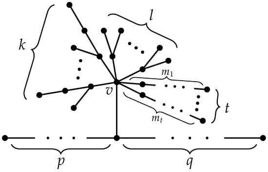
Figure 1. Structure of L-reflexive trees.

A nonsporadic L-reflexive tree contains a central vertex v with different branches emanating from it whose shape is illustrated in Figure 1. All $m_i$s and p, q values in the figure refer to the number of edges, whereas k, l, and t values refer to the number of corresponding branches. Some of the t-branches can also be unbounded, so their length is infinite.

The following criterion from ([12], Theorem 3.1) determines whether a tree in Figure 1 is L-reflexive.

Theorem 1.

Let T be a tree as in Figure 1. For some s and $j=0,1,\dots ,s$, denote by $t_j$ the number of $m_i$s equal to $j+1$, and by $t_{s+1}$ denote the number of infinite $m_i$s (i.e, the number of unbounded t-branches). Then, T is L-reflexive if and only if

$$4k+l+\sum _{i=0}^s\frac{i+1}{2i+3}{t}_i+\frac{1}{2}{t}_{s+1}\le \frac{p+q+1}{(2p-1)(2q-1)-4}+1,$$

(1)

where $1\le p\le q$ and $p+q\ge 4$.

It is also argued in [12] that we can simplify the left-hand side of Inequality (1) by taking $k=0$ and $l=0$, so Inequality (1) is reduced to

$$\sum _{i=0}^s\frac{i+1}{2i+3}{t}_i+\frac{1}{2}{t}_{s+1}\le \frac{p+q+1}{(2p-1)(2q-1)-4}+1.$$

(2)

Furthermore, from the discussion on the values of p and q in [12], it basically follows that the right-hand side of Inequality (2) can be taken to have discrete values, such as $6,3,2\frac{2}{5},2\frac{1}{7},2,\dots$. Thus, for one of these (fixed) discrete values of the right-hand side of Inequality (2), without losing too much generality, we can regard L-reflexive trees as trees having the canonical structure given in Figure 2.

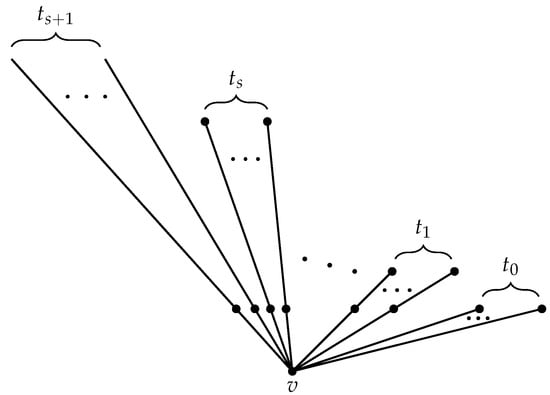
Figure 2. Canonical structure of L-reflexive trees.

To summarize, if

$$L=\sum _{i=0}^s\frac{i+1}{2i+3}{t}_i+\frac{1}{2}{t}_{s+1}$$

and $R=6,3,2\frac{2}{5},2\frac{1}{7},2,\dots$, then a canonical tree from Figure 2 is L-reflexive if and only if $L\le R$ for some $s\ge 0$, and some sequence $t_0,\dots ,t_s,t_{s+1}$ with each $t_i\ge 0$, where $i=0,\dots ,s,s+1$. Such an L-reflexive tree T is also maximal if adding one edge to any finite branch of the tree T makes its corresponding new sum L strictly greater than R.

The problem we are, therefore, interested in is: Given a fixed value $R=6,3,2\frac{2}{5},2\frac{1}{7},2,\dots$, generate all maximal L-reflexive trees with the canonical structure shown in Figure 2 (the number of such trees is finite, as shown in [4]).

Now, for $j=1,\dots ,s,s+1$, consider number of nodes $k_j$ at level j of the canonical tree from Figure 2. This is illustrated in Figure 3.

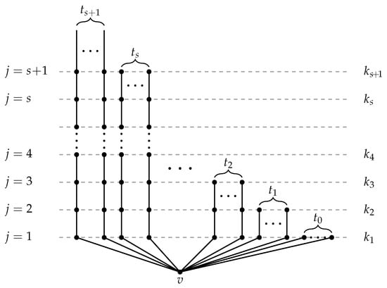
Figure 3. Levelled canonical structure of L-reflexive trees.

It is easy to see from Figure 3 that

$$k_j=\sum _{i=j-1}^{s+1}{t}_i,j=1,\dots ,s,s+1.$$

The next lemma shows that sum L for a canonical tree from Figure 2 can be computed in a different way using $k_j$s instead of $t_i$s as coefficients.

Lemma 1.

Let

$$L=\sum _{i=0}^s\frac{i+1}{2i+3}{t}_i+\frac{1}{2}{t}_{s+1}$$

for some $s\ge 0$ and some sequence $t_0,\dots ,t_s,t_{s+1}$ with each $t_i\ge 0$, $i=0,\dots ,s,s+1$. If $k_{s+2}=t_{s+1}$ and

$$k_j=\sum _{i=j-1}^{s+1}{t}_i,j=1,\dots ,s,s+1$$

then

$$L=\sum _{j=1}^{s+1}\frac{1}{(2j+1)(2j-1)}{k}_j+\frac{1}{2}{k}_{s+2}.$$

Proof. 

Since

$$\frac{1}{(2j+1)(2j-1)}=\frac{j}{2j+1}-\frac{j-1}{2j-1},j=1,\dots ,s+1,$$

telescoping gives

$$\begin{array}{cc}\hfill & \sum _{j=1}^{s+1}\frac{1}{(2j+1)(2j-1)}{k}_j+\frac{1}{2}{k}_{s+2}=\hfill \\ \hfill & \sum _{j=1}^{s+1}\left(\frac{j}{2j+1}-\frac{j-1}{2j-1}\right)\sum _{i=j-1}^{s+1}{t}_i+\frac{1}{2}{t}_{s+1}=\hfill \\ \hfill & \sum _{i=0}^s\frac{i+1}{2i+3}{t}_i+\frac{1}{2}{t}_{s+1}=L,\hfill \end{array}$$

as claimed. □

Coefficients $t_i$s can easily be recovered from coefficients $k_j$s, as the next lemma shows.

Lemma 2.

Let

$$L=\sum _{j=1}^{s+1}\frac{1}{(2j+1)(2j-1)}{k}_j+\frac{1}{2}{k}_{s+2}$$

for some $s\ge 0$ and some sequence $k_1,\dots ,k_{s+1},k_{s+2}$ such that $k_1\ge k_2\ge \cdots \ge k_{s+1}\ge k_{s+2}\ge 0$. If $t_{s+1}=k_{s+2}$ and $t_i=k_{i+1}-k_{i+2}$ for $i=0,\dots ,s$, then

$$L=\sum _{i=0}^s\frac{i+1}{2i+3}{t}_i+\frac{1}{2}{t}_{s+1}.$$

Proof. 

Similar telescoping technique. □

3. Algorithm

The basic idea of the algorithm for discovering a maximal L-reflexive tree (mlrt) having the structure given in Figure 2 is to use Lemma 1 to incrementally compute its corresponding sum L until it exceeds value R. Assuming for the moment that a maximal L-reflexive tree is finite, starting from $k_1$ nodes, $1\le k_1\le d$, at level 1, and going up level by level, at next level j we add $k_j\le k_{j-1}$ nodes (and edges) so that their total contribution, i.e., $k_j/\left((2j+1)(2j-1)\right)$, to already computed sum L does not exceed R. Clearly, if adding even one node at some level j makes already computed sum L greater than value R, then the tree encoded by sequence $k_1,\dots ,k_{j-1}$ is maximally L-reflexive.

The search space for all (finite and infinite) maximal L-reflexive trees is the set of all canonical trees from Figure 2. To facilitate systematic and efficient search, we modelled this space as an infinite tree with nodes representing subsets of all canonical trees from Figure 2. More precisely, the root of the search-space tree represents the set of all canonical trees from Figure 2, i.e., the set of such trees that have $k_1$ nodes on level 1, denote it by $T_{1,k_1}$. Set $T_{1,k_1}$ can be partitioned into mutually disjoint subsets $T_{2,k_1,k_1}$, $T_{2,k_1,k_1-1}$,…,$T_{2,k_1,1}$ of canonical trees having $k_1$, $k_1-1$, …, 1, respectively, nodes on level 2. Similarly, each set of trees $T_{2,k_1,m}$ on level 2, where $m=k_1,k_1-1,\dots ,1$, can be further divided into mutually disjoint subsets $T_{3,k_1,m,m}$, $T_{3,k_1,m,m-1}$, …, $T_{3,k_1,m,1}$ of canonical trees having m, $m-1$, …, 1, respectively, nodes on level 3. Continuing this procedure in the same fashion, we can thus represent the search space for all maximal L-reflexive trees from Figure 2 as a tree shown in Figure 4.

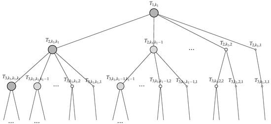
Figure 4. Search-space tree for maximal L-reflexive trees.

Figure 4 shows that set $T_{j,k_1,k_2,k_3,\dots ,k_j}$, where $k_1\ge k_2\ge k_3\ge \cdots \ge k_j\ge 1$, is represented by the subtree whose root is node $T_{j,k_1,k_2,k_3,\dots ,k_j}$ at level j on the path that starts from node $T_{1,k_1}$ on level 1. This path goes next to node $T_{2,k_1,k_2}$ on level 2, then to node $T_{3,k_1,k_2,k_3}$ on level 3, and so on. The path in this way ends with node $T_{j,k_1,k_2,k_3,\dots ,k_j}$ on level j. We also slightly abused our notation by using $T_{j,k_1,k_2,k_3,\dots ,k_j}$ to denote both a set of trees and a node in Figure 4 representing that set.

To each node $T_{j,k_1,k_2,\dots ,k_j}$ in Figure 4, we assigned a value $S\left(T_{j,k_1,k_2,\dots ,k_j}\right)=k_j$ and called it the node’s size, because $T_{j,k_1,k_2,\dots ,k_j}$ represents canonical trees that have $k_j$ nodes on level j. Different sizes of nodes are indicated in Figure 4 by the scaled diameters of the corresponding circles.

The following lemma is an immediate consequence of the construction of the search-space tree.

Lemma 3.

Let $T^{\prime }$ and $T^{″}$ be two canonical trees from Figure 2 and let $T^{\prime }\in T_{l,k_1,k_2^{\prime },\dots ,k_l^{\prime }}$ and $T^{″}\in T_{j,k_1,k_2^{″},\dots ,k_j^{″}}$. Then $T^{\prime }$ is a subtree of $T^{″}$ if and only if $l\le j$ and $k_i^{\prime }\le k_i^{″}$ for each $i=2,\dots ,l$.

We also assigned another value to each node $T_{j,k_1,k_2,\dots ,k_j}$ in Figure 4, called the node’s load, representing partial sum L accumulated when we follow the path going from the root to that node. In other words, node load $L=L(·)$ is computed recursively as

$$\begin{array}{cc}\hfill & L(T_{1,k_1)}=k_1/3,\hfill \\ \hfill & L\left(T_{j,k_1,k_2,\dots ,k_j}\right)=L\left(T_{j,k_1,k_2,\dots ,k_{j-1}}\right)+\frac{k_j}{(2j+1)(2j-1)},\hfill \end{array}$$

for $j=2,3,\dots$ and $1\le k_j\le k_{j-1}\le \cdots \le k_1\le d$.

We can now establish criteria for detecting whether a node of the search-space tree from Figure 4 represents a finite or infinite maximal L-reflexive tree. The first criterion for a finite maximal L-reflexive tree is obvious and stated here without proof.

Lemma 4.

A node $T_{j,k_1,k_2,\dots ,k_j}$ in Figure 4 represents a finite maximal L-reflexive tree encoded by sequence $k_1,k_2,\dots ,k_j$ if and only if its load L is not greater than R, and the load of all of its children is (strictly) greater than R.

On the other hand, whether a node of the tree from Figure 4 represents an infinite maximal L-reflexive tree can be determined using the following lemma.

Lemma 5.

Node $T_{j,k_1,k_2,\dots ,k_j}$ in Figure 4 represents an infinite L-reflexive tree encoded by sequence $k_1,k_2,\dots ,k_j$ if and only if its load L satisfies inequality

$$L+\frac{k_j}{2(2j+1)}\le R.$$

(3)

Proof. 

Node $T_{j,k_1,k_2,\dots ,k_j}$ on level j in Figure 4 represents an infinite L-reflexive tree if and only if for every $n\ge j$

$$L+\sum _{i=j}^n\frac{k_j}{(2i+3)(2i+1)}<R.$$

This inequality can be rewritten as

$$L+k_j·\left(\sum _{i=0}^n\frac{1}{(2i+3)(2i+1)}-\sum _{i=0}^{j-1}\frac{1}{(2i+3)(2i+1)}\right)<R$$

or

$$L+k_j·\left(\sum _{i=0}^n\frac{1}{(2i+3)(2i+1)}-\frac{j}{2j+1}\right)<R.$$

Letting $n\to \infty$ in the last inequality we get

$$L+k_j·\left(\frac{1}{2}-\frac{j}{2j+1}\right)\le R,$$

which is desired Inequality (3). □

We can use Lemma 5 to discover an infinite maximal L-reflexive tree if Inequality (3) is satisfied for the corresponding node in Figure 4 on the lowest level.

To now find all maximal L-reflexive trees, we can apply depth-first search to explore the search-space tree from Figure 4, computing the load of visited nodes along the way, and using Lemmas 4 and 5 to end a path from the root. However, we can actually do better by applying a kind of branch-and-bound technique to considerably cut the search space.

Namely, we first need to explore all children of a given node, but only those (if any) whose load does not exceed R. Clearly, the subtrees rooted at the children whose load already exceed R cannot possibly even contain L-reflexive trees, let alone maximal. The children whose load does not exceed R must be explored because the subtrees rooted in them each contain at least one maximal L-reflexive tree.

The second observation encompassed in the following lemma relates to nodes representing infinite maximal L-reflexive trees. Namely, Lemma 6 allows us to further cut the search space because, once a node representing an infinite maximal L-reflexive tree is found during depth-first search, all children nodes of its ancestors from the lemma can be ignored since they represent subtrees of the first-time-found infinite maximal L-reflexive tree.

Lemma 6.

Let node $T_{j,k_1,k_2,\dots ,k_j}$ in Figure 4 represent an infinite maximal L-reflexive tree, and for $l=1,\dots ,j-1$ consider any ancestor $T_{l,k_1,k_2,\dots ,k_l}$ of that node. Then, all children $T_{l+1,k_1,k_2,\dots ,k_l,k_l}$, $T_{l+1,k_1,k_2,\dots ,k_l,k_l-1}$, …, $T_{l+1,k_1,k_2,\dots ,k_l,1}$ of ancestor $T_{l,k_1,k_2,\dots ,k_l}$ also represent infinite L-reflexive trees.

Proof. 

By Lemma 3, children $T_{l+1,k_1,k_2,\dots ,k_l,k_l}$, $T_{l+1,k_1,k_2,\dots ,k_l,k_l-1}$, …, $T_{l+1,k_1,k_2,\dots ,k_l,1}$ of ancestor $T_{l,k_1,k_2,\dots ,k_l}$ are subtrees of $T_{j,k_1,k_2,\dots ,k_j}$. □

Previous considerations are incorporated into recursive algorithm mlrt given in Figure 5. Therefore, the following theorem is straightforward.

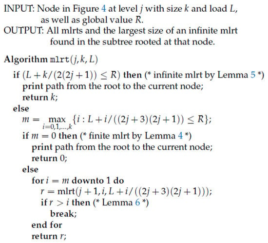
Figure 5. Maximal L-reflexive tree (mlrt) algorithm.

Theorem 2.

An initial call mlrt$(1,k_1,k_1/3)$for fixed $k_1\le d=\mathrm{deg}\left(v\right)$ and $R=6,3,2\frac{2}{5},2\frac{1}{7},2,\dots$ correctly generates all maximal L-reflexive trees from Figure 2.

4. Experiments

We tested our algorithm for the “hardest” cases of the right-hand side of Inequality (2), i.e., the five different values of $R=6,3,2\frac{2}{5},2\frac{1}{7},2$. For each value of R, we also used corresponding meaningful values for maximal degree d of central vertex v of a maximal L-reflexive tree from Figure 2. Results are shown in Table 1, where $N_{\mathrm{fin}}$ and $N_{\inf }$ denote the number of finite and infinite maximal L-reflexive trees, respectively. Not all rows in the table give exact values for $N_{\mathrm{fin}}$ and $N_{\inf }$, only their lower bounds, because the algorithm did not terminate in a reasonable amount of time due to a huge number of maximal L-reflexive trees.

Table 1. Number of maximal L-reflexive trees.

$R=6$	$d=18$:   $N_{\mathrm{fin}}=1,N_{\inf }=0$
	$d=17$:   $N_{\mathrm{fin}}=10,N_{\inf }=2$
	$d=16$:   $N_{\mathrm{fin}}=6474,N_{\inf }=131$
	$d=15$:   $N_{\mathrm{fin}}\ge 20310,N_{\inf }\ge 401$
	$d=14$:   $N_{\mathrm{fin}}\ge 13502,N_{\inf }\ge 254$
	$d=13$:   $N_{\mathrm{fin}}\ge 24957,N_{\inf }\ge 554$
	$d=12$:   $N_{\mathrm{fin}}=0,N_{\inf }=1$
$R=3$	$d=8$:   $N_{\mathrm{fin}}=10,N_{\inf }=2$
	$d=7$:   $N_{\mathrm{fin}}=6463,N_{\inf }=130$
	$d=6$:   $N_{\mathrm{fin}}=0,N_{\inf }=1$
$R=2\frac{2}{5}$	$d=7$:   $N_{\mathrm{fin}}=1,N_{\inf }=0$
	$d=6$:   $N_{\mathrm{fin}}=32,N_{\inf }=4$
	$d=5$:   $N_{\mathrm{fin}}\ge 28498,N_{\inf }\ge 298$
	$d=4$:   $N_{\mathrm{fin}}=0,N_{\inf }=1$
$R=2\frac{1}{7}$	$d=6$:   $N_{\mathrm{fin}}=2,N_{\inf }=0$
	$d=5$:   $N_{\mathrm{fin}}=590,N_{\inf }=17$
	$d=4$:   $N_{\mathrm{fin}}=0,N_{\inf }=1$
$R=2$	$d=6$:   $N_{\mathrm{fin}}=1,N_{\inf }=0$
	$d=5$:   $N_{\mathrm{fin}}=10,N_{\inf }=2$
	$d=4$:   $N_{\mathrm{fin}}=0,N_{\inf }=1$

5. Conclusions

In the paper, we considered L-reflexive trees that are those trees for which the second-largest eigenvalue of their line graph is at most 2. Previous work [4,12] showed that, apart from some sporadic examples, any L-reflexive tree is a subtree of a universal tree $T(k,l,t,m_1,\dots ,m_t;p,q)$ from Figure 1. The work in [4,12] also gave a criterion in the form of an inequality involving $k,l,t,m_i$’s,$p,q$ that precisely determines when these parameters yield an L-reflexive tree.

This paper used this inequality to devise an efficient recursive algorithm that searches for parameters that make the inequality true. In particular, the aim was to find maximal examples. The search has a natural rooted-tree structure, and some paths from the root may infinitely extend. These infinite trees can be neatly identified, in theory giving a finite search space.

References

- Cvetković, D.; Rowlinson, P.; Simić, S. Spectral Generalizations of Line Graphs: On Graphs with Least Eigenvalue −2; Cambridge University Press: Cambridge, UK, 2004. [Google Scholar]
- Cvetković, D.; Rowlinson, P.; Simić, S. An Introduction to the Theory of Graph Spectra; Cambridge University Press: Cambridge, UK, 2009. [Google Scholar]
- Cvetković, D.; Rowlinson, P.; Simić, S.K. Graphs with least eigenvalue −2: Ten years on. Linear Algebra Appl. 2015, 483, 504–539. [Google Scholar] [CrossRef]
- Simić, S.K.; Živković, D.; Anđelić, M.; da Fonseca, C.M. Reflexive line graphs of trees. J. Algebraic Combin. 2016, 43, 447–464. [Google Scholar] [CrossRef]
- Simić, S.K.; Anđelić, M.; da Fonseca, C.M.; Živković, D. Notes on the second largest eigenvalue of a graph. Linear Algebra Appl. 2015, 465, 262–274. [Google Scholar] [CrossRef]
- Maxwell, G. Hyperbolic trees. J. Algebra 1978, 54, 46–49. [Google Scholar] [CrossRef][Green Version]
- Neumaier, A. The second largest eigenvalue of trees. Linear Algebra Appl. 1982, 46, 2–25. [Google Scholar] [CrossRef]
- Radosavljević, Z. On unicyclic reflexive graphs. Appl. Anal. Discrete Math. 2007, 1, 228–240. [Google Scholar]
- Radosavljević, Z.; Simić, S. Which bicyclic graphs are reflexive? Fak. Ser. Mat. 1996, 7, 90–104. [Google Scholar]
- Rašajski, M.; Radosavljević, Z.; Mihailović, B. Maximal reflexive cactii with four cycles, The approach via Smith graphs. Linear Algebra Appl. 2011, 435, 2530–2543. [Google Scholar] [CrossRef]
- McKee, J.; Smyth, C. Salem Numbers, Pisot numbers, Mahler measure, and graphs. Exp. Math. 2005, 14, 211–229. [Google Scholar] [CrossRef]
- Anđelić, M.; Simić, S.K.; Živković, D. Reflexive line graphs of trees and Salem numbers. Mediterr. J. Math. 2019, 16, 127. [Google Scholar] [CrossRef]
© 2020 by the authors. Licensee MDPI, Basel, Switzerland. This article is an open access article distributed under the terms and conditions of the Creative Commons Attribution (CC BY) license (http://creativecommons.org/licenses/by/4.0/).