Criticality or Supersymmetry Breaking?

 , and
, and 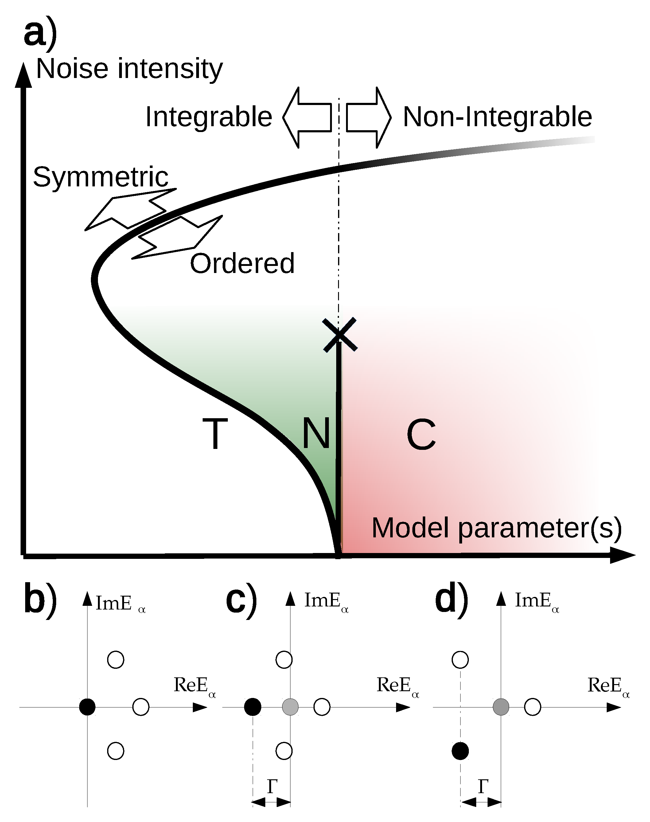
Abstract
1. Introduction
2. Basic Phase Diagram
2.1. 1D Chain of Stochastic Neuron-Like Elements
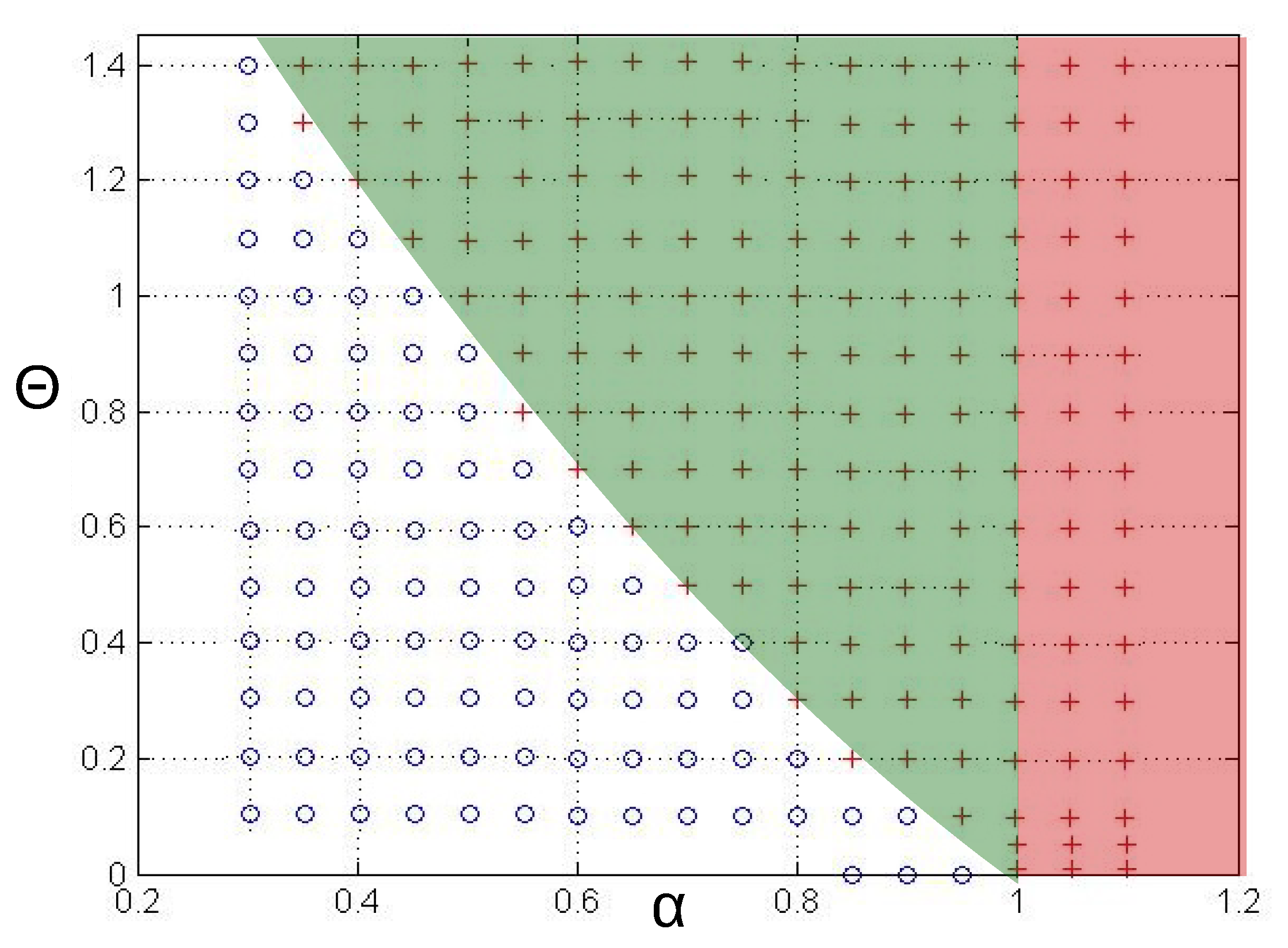
2.2. Stochastic Neurodynamics on Neuromorphic Hardware
Emulation Results
3. Neurodynamic Meaning of the Three Phases
Fine Structure
4. Conclusions
Author Contributions
Funding
Acknowledgments
Conflicts of Interest
Abbreviations
| DC | dynamical complexity |
| FVF | flow vector field |
| ND | neurodynamics |
| SDE | stochastic differential equation |
| SOC | self-organized criticality |
| STS | supersymmetric theory of stochastics |
| TS | topological supersymmetry |
Appendix A. Key Elements of Sts
Appendix A.1. The Model
Appendix A.2. From SDE to Topological Field Theory
Appendix A.3. Operator Representation
Appendix A.4. Eigensystem
Appendix A.5. Dynamical Partition Function, Supersymmetry Breaking, and Chaos
Appendix A.6. The Phase Diagram
References
- Aschwanden, M.J. Self-Organized Criticality in Astrophysics: The Statistics of Nonlinear Processes in the Universe; Springer: Berlin, Germany; New York, NY, USA, 2011. [Google Scholar]
- Preis, T.; Schneider, J.J.; Stanley, H.E. Switching processes in financial markets. Proc. Natl. Acad. Sci. USA 2011, 108, 7674–7678. [Google Scholar] [CrossRef] [PubMed]
- Gutenberg, B.; Richter, C.F. Magnitude and Energy of Earthquakes. Nature 1955, 176, 795. [Google Scholar] [CrossRef]
- Eldredge, N.; Gould, S. Punctuated equilibria: An alternative to phyletic gradualism. In Models in Paleobiology; Schopf, T., Ed.; Freeman, Cooper & Co.: San Francisco, CA, USA, 1972; pp. 82–115. [Google Scholar]
- Bialek, W.; Cavagna, A.; Giardina, I.; Mora, T.; Pohl, O.; Silvestri, E.; Viale, M.; Walczak, A.M. Social interactions dominate speed control in poising natural flocks near criticality. Proc. Natl. Acad. Sci. USA 2014, 111, 7212–7217. [Google Scholar] [CrossRef] [PubMed]
- Bialek, W.; Cavagna, A.; Giardina, I.; Mora, T.; Silvestri, E.; Viale, M.; Walczak, A.M. Statistical mechanics for natural flocks of birds. Proc. Natl. Acad. Sci. USA 2012, 109, 4786–4791. [Google Scholar] [CrossRef] [PubMed]
- Chialvo, D.R. Emergent complex neural dynamics. Nat. Phys. 2010, 6, 744–750. [Google Scholar] [CrossRef]
- Beggs, J.M.; Plenz, D. Neuronal Avalanches Are Diverse and Precise Activity Patterns That Are Stable for Many Hours in Cortical Slice Cultures. J. Neurosci. 2004, 24, 5216–5229. [Google Scholar] [CrossRef]
- Beggs, J.M.; Plenz, D. Neuronal Avalanches in Neocortical Circuits. J. Neurosci. 2003, 23, 11167–11177. [Google Scholar] [CrossRef]
- Musha, T.; Yamamoto, M. 1/f fluctuations in biological systems. Engineering in Medicine and Biology Society, 1997. In Proceedings of the 19th Annual International Conference of the IEEE, Chicago, IL, USA, 30 October–2 November 1997; Volume 6, pp. 2692–2697. [Google Scholar]
- Levina, A.; Herrmann, J.M.; Geisel, T. Dynamical synapses causing self-organized criticality in neural networks. Nat. Phys. 2007, 3, 857–860. [Google Scholar] [CrossRef]
- Bak, P.; Tang, C.; Wiesenfeld, K. Self-organized criticality: An explanation of the 1/ f noise. Phys. Rev. Lett. 1987, 59, 381–384. [Google Scholar] [CrossRef]
- Jensen, H.J.; Christensen, K.; Fogedby, H.C. 1/ f noise, distribution of lifetimes, and a pile of sand. Phys. Rev. B 1989, 40, 7425–7427. [Google Scholar] [CrossRef]
- Vespignani, A.; Zapperi, S. How self-organized criticality works: A unified mean-field picture. Phys. Rev. E 1998, 57, 6345–6362. [Google Scholar] [CrossRef]
- Watkins, N.W.; Pruessner, G.; Chapman, S.C.; Crosby, N.B.; Jensen, H.J. 25 Years of Self-organized Criticality: Concepts and Controversies. Space Sci. Rev. 2016, 198, 3–44. [Google Scholar] [CrossRef]
- Pruessner, G. Self-Organised Criticality; Cambridge University Press: Cambridge, UK, 2012. [Google Scholar]
- Frigg, R. Self-organised criticality—What it is and what it isn’t. Stud. Hist. Philos. Sci. Part A 2003, 34, 613–632. [Google Scholar] [CrossRef]
- Vespignani, A.; Zapperi, S. Order Parameter and Scaling Fields in Self-Organized Criticality. Phys. Rev. Lett. 1997, 78, 4793–4796. [Google Scholar] [CrossRef]
- Perković, O.; Dahmen, K.; Sethna, J.P. Avalanches, Barkhausen Noise, and Plain Old Criticality. Phys. Rev. Lett. 1995, 75, 4528–4531. [Google Scholar] [CrossRef] [PubMed]
- Christensen, K.; Moloney, N. Complexity and Criticality; Imperial College Press: London, UK, 2005. [Google Scholar]
- Massobrio, P.; de Arcangelis, L.; Pasquale, V.; Jensen, H.J.; Plenz, D. Criticality as a signature of healthy neural systems. Front. Syst. Neurosci. 2015, 9, 22. [Google Scholar] [CrossRef]
- Botcharova, M.; Farmer, S.F.; Berthouze, L. Markers of criticality in phase synchronization. Front. Syst. Neurosci. 2014, 8, 176. [Google Scholar] [CrossRef]
- Hesse, J.; Gross, T. Self-organized criticality as a fundamental property of neural systems. Front. Syst. Neurosci. 2014, 8, 166. [Google Scholar] [CrossRef]
- Roberts, J.A.; Iyer, K.K.; Vanhatalo, S.; Breakspear, M. Critical role for resource constraints in neural models. Front. Syst. Neurosci. 2014, 8, 154. [Google Scholar] [CrossRef]
- Bédard, C.; Kröger, H.; Destexhe, A. Does the 1/f Frequency Scaling of Brain Signals Reflect Self-Organized Critical States? Phys. Rev. Lett. 2006, 97, 118102. [Google Scholar] [CrossRef]
- Dehghani, N.; Hatsopoulos, N.; Haga, Z.; Parker, R.; Greger, B.; Halgren, E.; Cash, S.; Destexhe, A. Avalanche Analysis from Multielectrode Ensemble Recordings in Cat, Monkey, and Human Cerebral Cortex during Wakefulness and Sleep. Front. Physiol. 2012, 3, 302. [Google Scholar] [CrossRef]
- Priesemann, V.; Wibral, M.; Valderrama, M.; Pröpper, R.; Le Van Quyen, M.; Geisel, T.; Triesch, J.; Nikolić, D.; Munk, M.H.J. Spike avalanches in vivo suggest a driven, slightly subcritical brain state. Front. Syst. Neurosci. 2014, 8, 108. [Google Scholar] [CrossRef]
- Zare, M.; Grigolini, P. Criticality and avalanches in neural networks. Chaos Solitons Fractals 2013, 55, 80–94. [Google Scholar] [CrossRef]
- Tomen, N.; Rotermund, D.; Ernst, U. Marginally subcritical dynamics explain enhanced stimulus discriminability under attention. Front. Syst. Neurosci. 2014, 8, 151. [Google Scholar] [CrossRef]
- Obukhov, S.P. Self-organized criticality: Goldstone modes and their interactions. Phys. Rev. Lett. 1990, 65, 1395–1398. [Google Scholar] [CrossRef]
- LunBiao, X.; Bin, C.; MingXing, L. Goldstone Modes in Driven Diffusion Systems. Commun. Theor. Phys. 1999, 32, 229. [Google Scholar] [CrossRef]
- Ovchinnikov, I.V. Self-organized criticality as Witten-type topological field theory with spontaneously broken Becchi-Rouet-Stora-Tyutin symmetry. Phys. Rev. E 2011, 83, 051129. [Google Scholar] [CrossRef]
- Ovchinnikov, I.V. Introduction to Supersymmetric Theory of Stochastics. Entropy 2016, 18, 108. [Google Scholar] [CrossRef]
- Birmingham, D.; Blau, M.; Rakowski, M.; Thompson, G. Topological field theory. Phys. Rep. 1991, 209, 129. [Google Scholar] [CrossRef]
- Labastida, J.M.F. Morse theory interpretation of topological quantum field theories. Commun. Math. Phys. 1989, 123, 641–658. [Google Scholar] [CrossRef]
- Witten, E. Topological quantum field theory. Commun. Math. Phys. 1988, 117, 353–386. [Google Scholar] [CrossRef]
- Witten, E. Topological sigma models. Commun. Math. Phys. 1988, 118, 411–449. [Google Scholar] [CrossRef]
- Blau, M. The Mathai-Quillen formalism and topological field theory. J. Geom. Phys. 1993, 11, 95–127. [Google Scholar] [CrossRef]
- Baulieu, L.; Grossman, B. A topological interpretation of stochastic quantization. Phys. Lett. B 1988, 212, 351. [Google Scholar] [CrossRef]
- Baulieu, L.; Singer, M. The topological sigma model. Commun. Math. Phys. 1989, 125, 227. [Google Scholar] [CrossRef]
- Slavik, A. Generalized differential equations: Differentiability of solutions with respect to initial conditions and parameters. J. Math. Anal. Appl. 2013, 402, 261–274. [Google Scholar] [CrossRef]
- Ovchinnikov, I.V.; Schwartz, R.N.; Wang, K.L. Topological supersymmetry breaking: The definition and stochastic generalization of chaos and the limit of applicability of statistics. Mod. Phys. Lett. B 2016, 30, 1650086. [Google Scholar] [CrossRef]
- Ovchinnikov, I.V.; Di Ventra, M. Chaos or Order ? arXiv 2017, arXiv:1702.06561. [Google Scholar]
- Lorenz, E. Deterministic nonperiodic flow. J. Atmos. Sci. 1963, 20, 130. [Google Scholar] [CrossRef]
- Gilmore, R. Topological analysis of chaotic dynamical systems. Rev. Mod. Phys. 1998, 70, 1455. [Google Scholar] [CrossRef]
- Witten, E. Dynamical breaking of supersymmetry. Nucl. Phys. B 1981, 188, 513–554. [Google Scholar] [CrossRef]
- Pfeil, T.; Grübl, A.; Jeltsch, S.; Müller, E.; Müller, P.; Petrovici, M.A.; Schmuker, M.; Brüderle, D.; Schemmel, J.; Meier, K. Six Networks on a Universal Neuromorphic Computing Substrate. Front. Neurosci. 2013, 7, 11. [Google Scholar] [CrossRef] [PubMed]
- Pfeil, T.; Jordan, J.; Tetzlaff, T.; Grübl, A.; Schemmel, J.; Diesmann, M.; Meier, K. Effect of Heterogeneity on Decorrelation Mechanisms in Spiking Neural Networks: A Neuromorphic-Hardware Study. Phys. Rev. X 2016, 6, 021023. [Google Scholar] [CrossRef]
- Quintero, N.R.; Sánchez, A.; Mertens, F.G. Overdamped sine-Gordon kink in a thermal bath. Phys. Rev. E 1999, 60, 222–230. [Google Scholar] [CrossRef] [PubMed]
- Eilenberger, G. BREMSSTRAHLUNG FROM SOLITONS. Z. Phys. B Condens. Matter 1977, 27, 199–203. [Google Scholar] [CrossRef]
- Lomdahl, P.S.; Soerensen, O.H.; Christiansen, P.L. Soliton excitations in Josephson tunnel junctions. Phys. Rev. B 1982, 25, 5737–5748. [Google Scholar] [CrossRef]
- Braun, O.M.; Kivshar, Y.S. Nonlinear dynamics of the Frenkel–Kontorova model. Phys. Rep. 1998, 306, 1–108. [Google Scholar] [CrossRef]
- Hermon, Z.; Ben-Jacob, E.; Schön, G. Charge solitons in one-dimensional arrays of serially coupled Josephson junctions. Phys. Rev. B 1996, 54, 1234–1245. [Google Scholar] [CrossRef]
- Pesin, Y. Characteristic Lyapunov exponents and smooth ergodic theory. Russ. Math. Surv. 1977, 32, 55–114. [Google Scholar] [CrossRef]
- Arnold, L. Lyapunov Exponents of Nonlinear Stochastic Systems. In Nonlinear Stochastic Dynamic Engineering Systems: IUTAM Symposium Innsbruck Igls, Austria, 21–26 June 1987; Ziegler, F., Schuëller, G.I., Eds.; Springer: Berlin/Heidelberg, Germany, 1988; pp. 181–201. [Google Scholar]
- Grassberger, P.; Badii, R.; Politi, A. Scaling laws for invariant measures on hyperbolic and nonhyperbolic atractors. J. Stat. Phys. 1988, 51, 135–178. [Google Scholar] [CrossRef]
- Hudson, A.E.; Calderon, D.P.; Pfaff, D.W.; Proekt, A. Recovery of consciousness is mediated by a network of discrete metastable activity states. Proc. Natl. Acad. Sci. USA 2014, 111, 9283–9288. [Google Scholar] [CrossRef] [PubMed]
- Ries, C.R.; Puil, E. Mechanism of Anesthesia Revealed by Shunting Actions of Isoflurane on Thalamocortical Neurons. J. Neurophysiol. 1999, 81, 1795–1801. [Google Scholar] [CrossRef] [PubMed]
- Touboul, J.; Destexhe, A. Can Power-Law Scaling and Neuronal Avalanches Arise from Stochastic Dynamics? PLoS ONE 2010, 5, e8982. [Google Scholar] [CrossRef] [PubMed]
- Meisel, C.; Storch, A.; Hallmeyer-Elgner, S.; Bullmore, E.; Gross, T. Failure of adaptive self-organized criticality during epileptic seizure attacks. PLoS Comput. Biol. 2012, 8, e1002312. [Google Scholar] [CrossRef]
- Beck, J.M.; Ma, W.J.; Pitkow, X.; Latham, P.E.; Pouget, A. Not Noisy, Just Wrong: The Role of Suboptimal Inference in Behavioral Variability. Neuron 2012, 74, 30–39. [Google Scholar] [CrossRef]
- Deco, G.; Rolls, E.T.; Romo, R. Stochastic dynamics as a principle of brain function. Prog. Neurobiol. 2009, 88, 1–16. [Google Scholar] [CrossRef]
- Rolls, E.T.; Webb, T. Cortical attractor network dynamics with diluted connectivity. Brain Res. 2012, 1434, 212–225. [Google Scholar] [CrossRef]
- Wilson, H.R.; Cowan, J.D. Excitatory and Inhibitory Interactions in Localized Populations of Model Neurons. Biophys. J. 1972, 12, 1–24. [Google Scholar] [CrossRef]
- Siettos, C.; Starke, J. Multiscale modeling of brain dynamics: From single neurons and networks to mathematical tools. Wiley Interdiscip. Rev. Syst. Biol. Med. 2016, 8, 438–458. [Google Scholar] [CrossRef]
- Freedman, M.H.; Kitaev, A.; Larsen, M.J.; Wang, Z. Topological quantum computation. Bull. Am. Math. Soc. 2003, 40, 31–38. [Google Scholar] [CrossRef]
- Parisi, G.; Sourlas, N. Supersymmetric field theories and stochastic differential equations. Nucl. Phys. B 1982, 206, 321. [Google Scholar] [CrossRef]
- Zinn-Justin, J. Renormalization and stochastic quantization. Nucl. Phys. B 1986, 275, 135–159. [Google Scholar] [CrossRef]
- Drummond, I.; Horgan, R. Stochastic processes, slaves and supersymmetry. J. Phys. A 2012, 45, 095005. [Google Scholar] [CrossRef]
- Witten, E. Supersymmetry and Morse theory. J. Differ. Geom. 1982, 17, 661–692. [Google Scholar] [CrossRef]
- Itô, K. Stochastic integral. Proc. Imp. Acad. 1944, 20, 519–524. [Google Scholar] [CrossRef]
- Stratonovich, R. A new representation for stochastic integrals and equations. SIAM J. Contr. 1966, 4, 362–371. [Google Scholar] [CrossRef]
- von Kampen, N. Itó versus Stratonovich. J. Stat. Phys. 1981, 24, 175–187. [Google Scholar] [CrossRef]
- Mostafazadeh, A. Pseudo-Hermiticity versus PT-symmetry III: Equivalence of pseudo-Hermiticity and the presence of anti-linear symmetries. J. Math. Phys. 2002, 43, 3944–3951. [Google Scholar] [CrossRef]
- Ovchinnikov, I.V.; Enßlin, T.A. Kinematic dynamo, supersymmetry breaking, and chaos. Phys. Rev. D 2016, 93, 085023. [Google Scholar] [CrossRef]
- Li, K.; Livermore, P.W.; Jackson, A. An optimal Galerkin scheme to solve the kinematic dynamo eigenvalue problem in a full sphere. J. Comput. Phys. 2010, 229, 8666–8683. [Google Scholar] [CrossRef]
- Lerche, I. Kinematic-Dynamo Theory. Astrophys. J. 1971, 166, 62. [Google Scholar] [CrossRef]
- Roberts, P.H. Kinematic Dynamo Models. R. Soc. Lond. Philos. Trans. Ser. A 1972, 272, 663–698. [Google Scholar]
- Bouya, I.; Dormy, E. Revisiting the ABC flow dynamo. Phys. Fluids 2013, 25, 037103. [Google Scholar] [CrossRef]
- Ott, E. Lagrangian chaos and the fast kinematic dynamo problem. In Chaos, Kinetics and Nonlinear Dynamics in Fluids and Plasmas, Proceedings of a Workshop Held in Carry-Le Rouet, France, 16–21 June 1997; Benkadda, S., Zaslavsky, G.M., Eds.; Springer: Berlin/Heidelberg, Germany, 1998; pp. 263–274. [Google Scholar]
- Adler, R.; Konheim, A.; Mc Andrew, M. Topological entropy. Trans. Am. Math. Soc. 1965, 114, 309. [Google Scholar] [CrossRef]


© 2020 by the authors. Licensee MDPI, Basel, Switzerland. This article is an open access article distributed under the terms and conditions of the Creative Commons Attribution (CC BY) license (http://creativecommons.org/licenses/by/4.0/).
Share and Cite
Ovchinnikov, I.V.; Li, W.; Sun, Y.; Hudson, A.E.; Meier, K.; Schwartz, R.N.; Wang, K.L. Criticality or Supersymmetry Breaking? Symmetry 2020, 12, 805. https://doi.org/10.3390/sym12050805
Ovchinnikov IV, Li W, Sun Y, Hudson AE, Meier K, Schwartz RN, Wang KL. Criticality or Supersymmetry Breaking? Symmetry. 2020; 12(5):805. https://doi.org/10.3390/sym12050805
Chicago/Turabian StyleOvchinnikov, Igor V., Wenyuan Li, Yuquan Sun, Andrew E. Hudson, Karlheinz Meier, Robert N. Schwartz, and Kang L. Wang. 2020. "Criticality or Supersymmetry Breaking?" Symmetry 12, no. 5: 805. https://doi.org/10.3390/sym12050805
APA StyleOvchinnikov, I. V., Li, W., Sun, Y., Hudson, A. E., Meier, K., Schwartz, R. N., & Wang, K. L. (2020). Criticality or Supersymmetry Breaking? Symmetry, 12(5), 805. https://doi.org/10.3390/sym12050805