Article

An Imbalanced Data Handling Framework for Industrial Big Data Using a Gaussian Process Regression-Based Generative Adversarial Network

School of Industrial Engineering, Kumoh National Institute of Technology, Gumi 39177, Korea
*
Author to whom correspondence should be addressed.
Symmetry 2020, 12(4), 669; https://doi.org/10.3390/sym12040669
Submission received: 20 March 2020 / Revised: 17 April 2020 / Accepted: 20 April 2020 / Published: 23 April 2020

Abstract

:
The developments in the fields of industrial Internet of Things (IIoT) and big data technologies have made it possible to collect a lot of meaningful industrial process and quality-based data. The gathered data are analyzed using contemporary statistical methods and machine learning techniques. Then, the extracted knowledge can be used for predictive maintenance or prognostic health management. However, it is difficult to gather complete data due to several issues in IIoT, such as devices breaking down, running out of battery, or undergoing scheduled maintenance. Data with missing values are often ignored, as they may contain insufficient information from which to draw conclusions. In order to overcome these issues, we propose a novel, effective missing data handling mechanism for the concepts of symmetry principles. While other existing methods only attempt to estimate missing parts, the proposed method generates a whole set of data set using Gaussian process regression and a generative adversarial network. In order to prove the effectiveness of the proposed framework, we examine a real-world, industrial case involving an air pressure system (APS), where we use the proposed method to make quality predictions and compare the results with existing state-of-the-art estimation methods.

1. Introduction

Failure analysis and process predictions for manufacturing processes have significant impacts on improving product quality and process reliability. A number of studies on failure cause analysis and classification using machine learning or deep learning methods are actively been conducted, which will lead to improvements in product quality and reliability. For instance, a failure of the brakes in a vehicle may lead to a significant accident, so it is important to predict any potential failures. In heavy vehicles such as trucks excavators, the performance of the brakes is very important due to the heavy weight they must bring to a halt. The brakes of a truck are driven by an air pressure system, and therefore require pressurized air to operate. If the air pressure in the system does not reach a certain level, its brakes may not work precisely and then serious accidents can occur. This research focuses on quality prediction of an air compressor and pressure system found in vehicles. The air pressure system (APS), an essential part of the vehicle, stops or decelerates the vehicle by applying compressed air to the brakes. Figure 1 depicts the APS structure.
As shown in Figure 1, the air compressor compresses air that is initially at atmospheric pressure and maintains the air at optimum pressure through the air compressor governor. The compressed air moves to the air reservoir. When the driver presses the brake pedal, the brake valve closes and compressed air stored in the air reservoir is used to brake by applying pressure to the brake chamber through the line.
It is important to predict defects and malfunctions in the APS. Well considered analysis of data leads to reliable predictions of potential APS failures and contributes to the minimization of dangers, as well as reduces maintenance costs. In this study, the data set for the failure analysis is from APS operations and the relevant quality data is from the Scania trucks data set [1]. This data set consists of the operating sensor attributes from a broken Scania truck, in which the attributes are anonymized. In order to investigate the causes of any APS failure, these attributes and their data are analyzed using several machine learning and statistical methods.
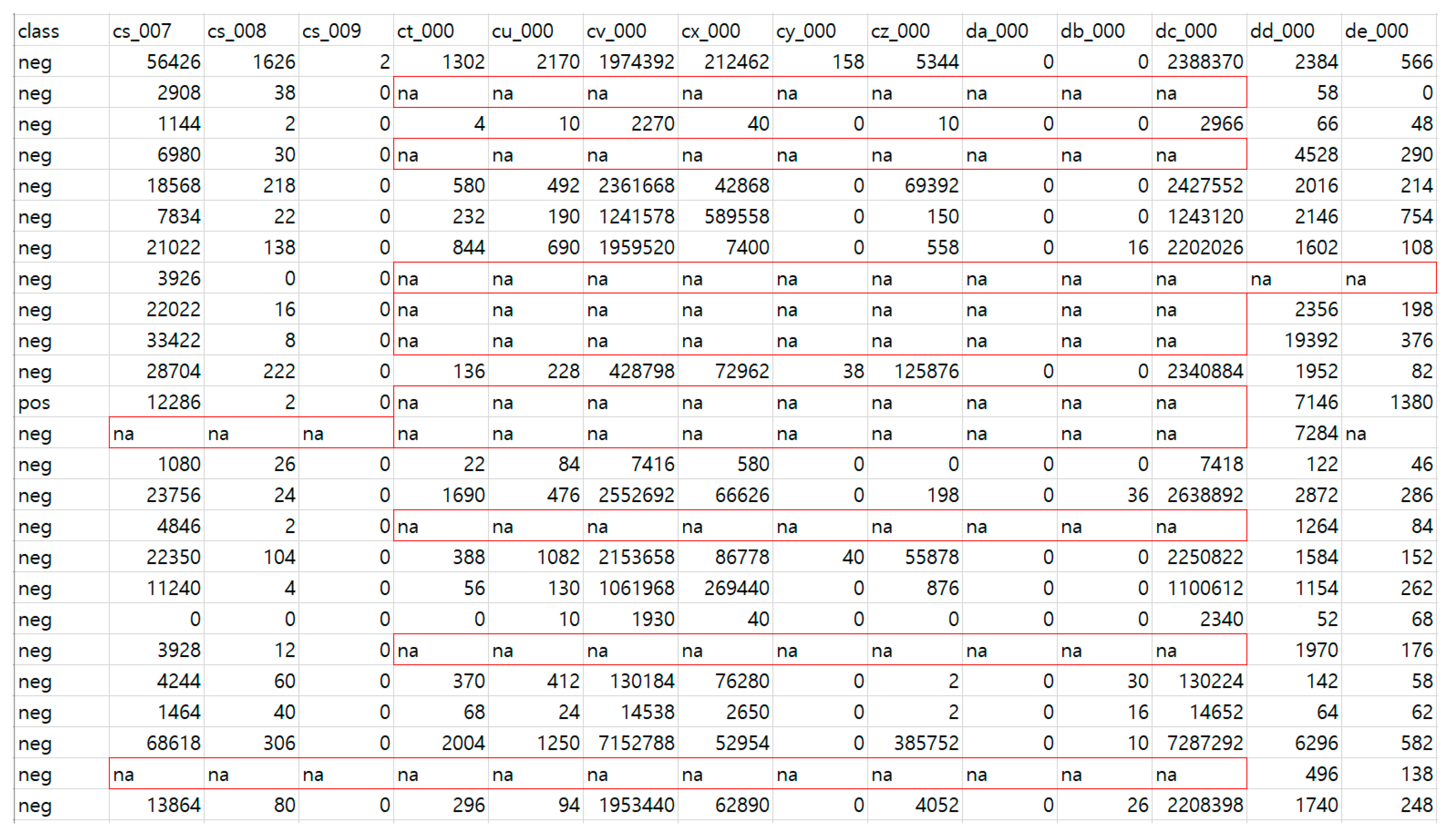
However, the data have a number of missing values due to sensor failures. Missing data can mean that there is insufficient information for analysis by existing methods and can make it difficult to identify the actual cause of any failure. In addition, missing values cause disproportionately distributed data, and for models trained on properly proportioned data this reduces the accuracy of the classification performance. Figure 2 shows the issue of missing values in a real APS failure incident in the Scania trucks data set. Missing values are marked as not available (na). The data are used for the failure study of a vehicle. The positive class (pos) of the data set indicates that the failure is in the APS, and the negative class (neg) indicates that the failure is not related to the APS.
In APS failure analysis, the classification performance depends heavily on the data’s completeness level. The more missing values in the data, the lower the completeness level is. Unfortunately, the Scania APS data contains a number of missing values. In addition, these missing values may cause a lack of data for analysis. Therefore, it is important to have a framework that handles incomplete data. Missing values and data imbalances are a primary cause for less accurate quality prediction. In addition, several kinds of multivariate statistical analysis cannot be applied to this data set due to the issues of missing values. This situation makes missing value estimations the most important preprocessing steps. A number of existing studies [2,3,4,5,6,7,8,9,10,11,12,13] have proposed methods to overcome this data imbalance issue. Table 1 summarizes several existing missing value estimation methods and their applications.
Most research methods resort to data imputation, where a data set with missing values is ignored. However, these kinds of methods cause distortion of the captured data-based probability distribution. In addition, the variance of the data that is used becomes heavily distorted. In order to overcome the issue, this paper proposes a novel, effective framework to generate a complete data set using a generative adversarial network (GAN) and Gaussian processes regression (GPR). The proposed framework is based on the symmetry principles, which the original data and the generated data have. Scania APS data are used as exemplary test data and the proposed method is compared with other existing methods.
Section 2 examines the background of the key techniques we use (GPR and GAN) and reviews the relevant literature. Section 3 proposes an overall framework for generating a data set using GPR and GAN. Section 4 shows the proposed method’s effectiveness with experimental analysis of the proposed framework and provides comparisons with other classification models using the APS data.

2. Background Knowledge and Literature Reviews

2.1. Gaussian Processes Regression

GPR [15,16,17,18,19] is a Bayesian algorithm and has the ability to provide a statistical uncertainty measure. Since it can provide high uncertainty prediction measurements in changing environments, the GPR algorithm has been applied in various research fields, as shown in Table 2.
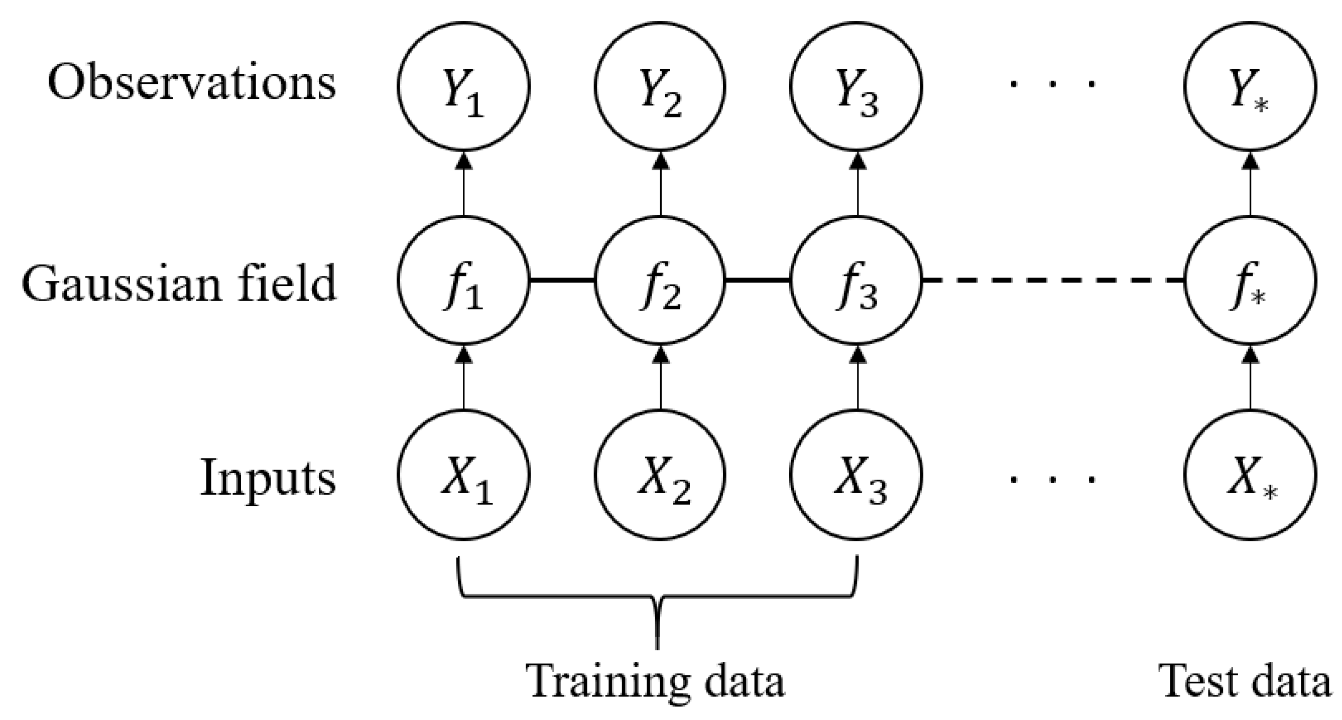
Figure 3 depicts the general process of GPR. The latent variable f i is derived from the input value X i with the observed value Y i . The distribution of the test observation value Y * is estimated using the Gaussian field f * for the input value X * .
The training data set is { ( x ( i ) , y ( i ) ) } i = 1 l , while Equations (1) and (2) summarize the general GPR model.
y = f + ϵ
where, ϵ   ~   N ( 0 , σ y 2 I )
f   ~   GP ( m ( x ) , k ( x , x * ) )
where m ( x ) = E [ f ( x ) ] , and   k ( x , x * ) = E [ ( f ( x ) m ( x ) ) ( f ( x * ) m ( x * ) ) ] .
In Equation (1), ϵ is a noise parameter that follows a Gaussian distribution, with variance of σ y 2 and a mean of 0. Here, I is an identity matrix constructed according to the data’s dimensions, f is the transformation relation-based value for the equivalent input vector X, and Y is the observed output vector. Equation (2) is the “distribution over functions” [19] used to derive the test target value Y using the Gaussian model. The distribution consists of a mean m ( x ) and variance covariance k ( x , x * ) derived by sampling from a multivariate Gaussian distribution. The covariance function k ( x , x * ) is commonly parameterized by a kernel parameter and models the dependence between existing observed input points x and new test input points to predict x * . Equation (3) is a radial basis kernel function that calculates a similarity measure between both data instances. The kernel is a closeness measure of data points. It is not just used to model the dependence of observed and unobserved points, but all points.
k ( x , x * ) = exp ( γ | x x * | 2 )
where   γ is a hyper parameter of the kernel function.
The parameter γ is related with the variance of a data set. After the mean function and kernel types are selected, the Gaussian process produce predictions are made based on previous observations. However, any actual data obtained from measurements include a lot of noise in general. Therefore, an observed output vector Y with its noise is expressed as in Equation (4).
Y ~ N ( 0 , k + σ y 2 I )
In Equation (4), the observed output vector Y with a mean 0 and covariance k + σ y 2 I follows the properties of multivariate Gaussian distribution and is used as a prediction model. Equation (5) denotes the prior distribution for f * ( X * ) with the noise condition, f * ( X * ) is a function that outputs a predicted vector Y * for a vector X * , which has a new input point x * . It is a prior distribution model that considers the noise generated when the test data vector X * is input and the output data are predicted through the function value f * ( X * ) .
[ Y f * ] ~ N ( 0 , [ k ( X , X ) + σ y 2 I      k ( X , X * )       k ( X * , X )             k ( X * , X * ) ] )
The maximum likelihood estimator (MLE) and variance of the predicted distribution derived using the newly updated Gaussian process is expressed as seen in Equations (6) and (7).
m ( x ) = k ( x , X ) ( k ( X , X ) + σ y 2 I ) 1 Y
k ( x , x * ) = k ( x , x * ) k ( x , X ) ( k ( X , X ) + σ y 2 I ) 1 k ( X , x * )
In this study, the introduced GPR framework is used to estimate missing values in our real-world imbalanced data set. The GPR process helps produce more accurate modeling from the data. The following section explains the GAN method, which generates a new data set using the GPR-based missing value estimations.

2.2. Generative Adversarial Network

GAN [27] is a generative model that uses the neural network architecture. A general GAN framework includes two types of model, both of which are neural networks: a generator (G) and a discriminator (D). Both models generate data that become closer to the real data set by competing with each other. GANs have been used in many research fields, as shown in Table 3.
As shown in Figure 4, the generator G takes a vector z extracted from random noise as its input and attempts to generate data which is close to the real data. The discriminator D learns how to distinguish between real data and the generated fake data. During training, while this process is being repeated, the generator minimizes the probability that the discriminator can distinguish real from generated data, and the discriminator maximizes the probability of distinguishing real data from the generated data.
As shown in Figure 4, the sample data extracted from the real data are represented by x and the distribution of the real data are p d a t a ( x ) . The distribution of the data from the generator is p g and the input noise variable is p g ( z ) . The discriminator and the generator are differential multilayer perceptrons with θ d and θ g as parameters, respectively.
D ( x ) is the probability that x comes from the real data distribution. D ( G ( z ) ) is the probability that G ( z ) comes from the p g , which is not from the real data distribution. D ( x ) should point to 1 and D ( G ( z ) ) should point to 0, resulting in a min-max problem as shown in Equation (8). The objective function of GAN is shown in Equation (8).
min G   max D V ( D , G ) = E x ~ p d a t a ( x ) [ log D ( x ) ] + E z ~ p z ( z ) [ log ( 1 D ( G ( z ) ) ) ]
where f D ( x d ) = E x ~ p d a t a ( x ) [ log D ( x ) ] ,   f G ( x g ) = E z ~ p z ( z ) [ log ( 1 D ( G ( z ) ) ) ] .
According to the distributions ( p g and p d a t a ( x ) ), the discriminator learns to distinguish between the real and the fake, and the generator also learns to produce a distribution that is similar to the real data in order to prevent the discriminator from easily distinguishing what is fake. If this learning process is repeated, p g = p d a t a ( x ) , so we get to the point where the discriminator cannot distinguish anymore. Then, the converged D ( x ) follows Equation (9).
D * ( x ) = p d a t a ( x ) p d a t a ( x ) + p g ( x )
In Equation (8), the optimum value is obtained at p g = p d a t a ( x ) so, the value of D * ( x ) is 1 2 . The generator proceeds learning in a way so that D * ( x ) becomes close to 1 2 .
This research applies the GAN framework, which is used for the correction of missing data after GPR correction. The detailed framework is provided in Section 3.

3. Generative Adversarial Network-Based Missing Value Estimation Framework

In general, real data from manufacturing processes contains a number of missing values. This causes a lack of data and data imbalance as a result. These issues such as data shortages and data imbalances make it difficult to analyze the industrial data accurately. This section explains a new and effective framework to estimate the missing values and generate data that is closer to the real data distribution. Figure 5 shows the detailed procedures for generating a data set, which includes missing values.
As shown in Figure 5, the missing values of the original data are indicated as not available (na). First, if na exists, it is replaced with the average value of the attribute data that are missing. The average value e h l is derived according to Equation (10).
e h l = h = 1 n a h n
where n is the number of remaining values, except for the missing value in the attribute, where the missing value comes from; h is the number of instance vectors and l is the number of attributes.
Then, approximate estimation of the missing value is achieved using GPR. In this case, GPR is applied to an instance vector.
f ( Y * ) ~ N ( m ( X ) , k ( X , X * ) )
Equation (11) is derived using the prediction procedure provided in Section 2.1. The missing value is estimated by predicting a new estimate Y * through Equations (12)–(14). Missing values are predicted based on GPR and updated to e h l .
X = [ x h 1 , x h 2 , , e h k , x h l ]
f ( e h k ) ~ N ( [ m ( e h k ) ] , [ k ( X k , X 1 ) k ( X k , X l ) ] )
p h k = Y k = f ( e h k ) + ϵ
In Equation (12), X is an input vector with l attributes and k is the missing index among these attributes. Equation (13) is the distribution of the latent variables in the k t h attribute where the missing value occurs, and the missing value correction value p h k using GPR is the same as Equation (13). Then, the e h k is transformed to Y k using Equation (14).
Finally, GAN is used to estimate missing values. The discriminator distinguishes the real instance vector distribution from the generated instance vector distribution, and the generator produces a new instance vector distribution based on the error generated by the discriminator.
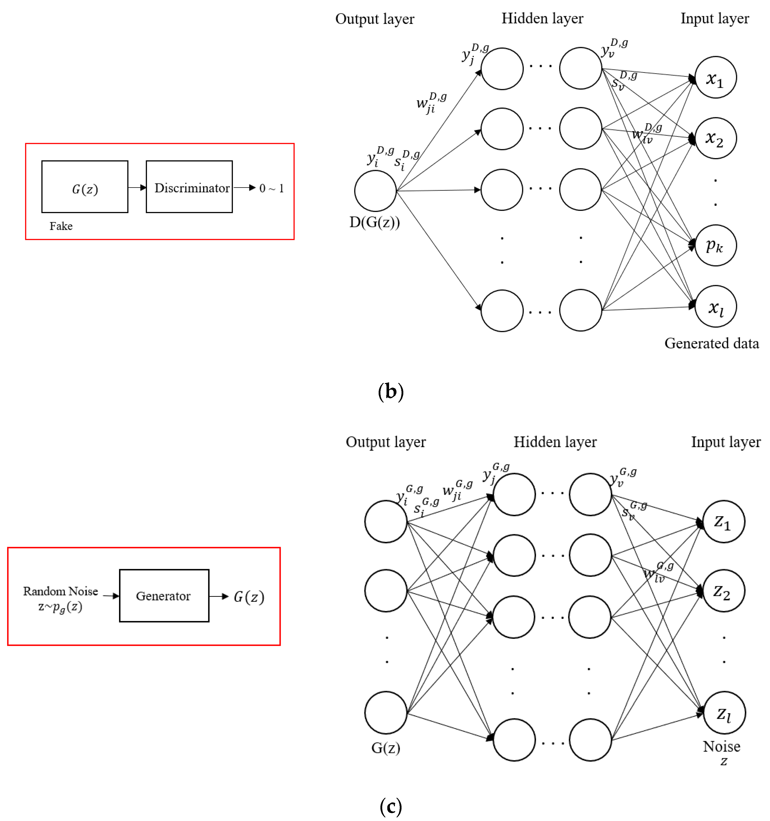
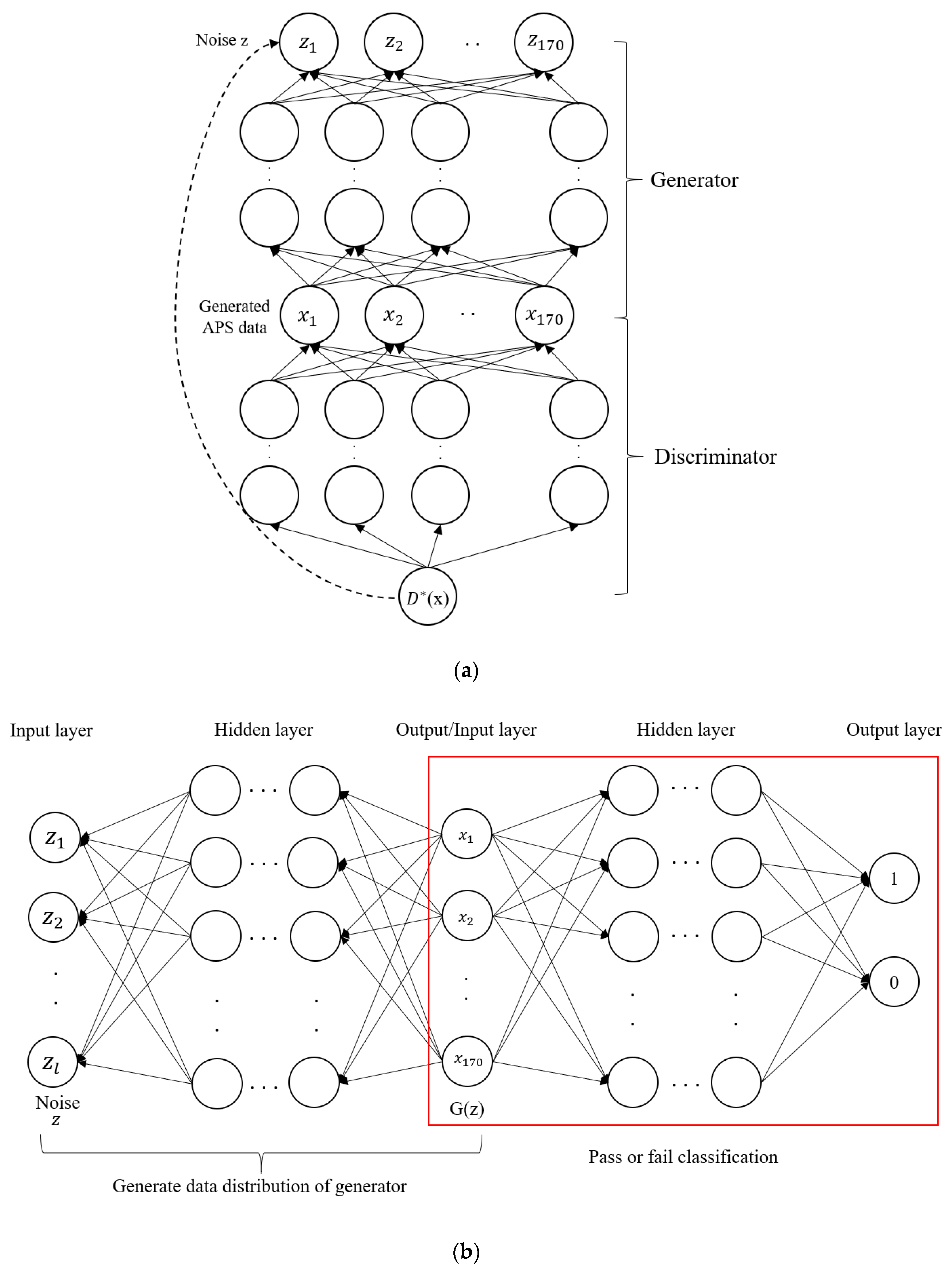
The discriminator derives gradients using the backpropagation algorithm to maximize Equation (8), while the generator derives the relevant gradient using the backpropagation algorithm to minimize f G ( x g ) during the learning process. In this study, the gradient is derived to maximize E z ~ p z ( z ) [ log ( D ( G ( z ) ) ) ] to increase the convergence speed of learning. The learning process using the backpropagation algorithm for the discriminator and generator is shown in Figure 6.
Figure 6a shows the discriminator’s learning process that is used to distinguish whether the input data are from real data or are generated data. Figure 6b shows the learning process of a discriminator to distinguish whether the input data are real or not. Figure 6c shows the learning process in which the generator generates data from random noise values.
V θ ( D ) = f ( x d ) θ ( D ) + f ( x g ) θ ( D )
f D ( x d ) w j i D , d = f D ( x d ) y i D , d · y i D , d s i D , d s v D , d w j i D , d
f D ( x d ) w N j D , d = 1 D ( x ) · ( y i D , d ) · w j i D , d · ( y j D , d ) · x d ,   f G ( x g ) w j i D , g = f G ( x g ) y i D , g · y i D , g s i D , g s v D , g w j i D , g
f G ( x g ) w N j D , g = 1 1 D ( G ( z ) ) · ( y i D , g ) · w j i D , g · ( y j D , g ) · x g ,   V θ ( G ) = f G ( x g ) θ ( G )
f G ( x g ) w j i G , g = f G ( x g ) y i G , g · y i G , g s i G , g s v G , g w j i G , g ,   f G ( x g ) w N j G , g = 1 D ( G ( z ) ) · ( y i G , g ) · w j i G , g · ( y j G , g ) · z
where y i = 1 1 + e s i ,   s i = N = 1 y i w j i   y j = 1 1 + e s j ,   s j = N = 1 y j w N j .
Equations (15)–(17) summarize the backpropagation processes of the discriminator, and Equation (18) and Equation (19) summarize the backpropagation process of the generator. The backpropagation process of the discriminator derives the gradients for D ( x ) and D ( G ( z ) ) , as shown in respective Equation (16) and Equation (17).
w is the weight of the neural network, and the sigmoid function is used as its activation function in this paper. Based on the output derived by the discriminator learning, the generator updates w through the gradient to produce a newly generated data. When D ( x ) converges through repetition, the estimation process is terminated.
X = [ x h 1 , x h 2 , , p h k , x h l ]
f G ( x g ) X = 1 D ( G ( z ) ) · ( y i G , g ) · w j i G , g · ( y j G , g ) · z
The missing value p h k in Equation (20) is estimated and a new data set is generated using Equation (21). Using these processes, a new set of data are generated. The generated data are considered balanced data.
In order to show the effectiveness of GPR-based GAN, time series data with missing values were tested. Figure 7a shows original time-series data, including Autoregressive Moving-Average (ARMA) model - ARMA(1,1) with the Gaussian noise N(0,2). The number of data points is 1024 (N = 1024). Among them, 100 points are randomly picked as missing parts.
Then, GPR-GAN is applied to estimate the missing value. Figure 7b shows the data gap between the original data and the newly generated data. In order to measure the accuracy of the generated method, Equation (22) is applied.
Accuracy   ( % ) = ( 1 i = 1 N O i G i O i ) 100
The proposed method has 91.23% accuracy in the provided numerical test.
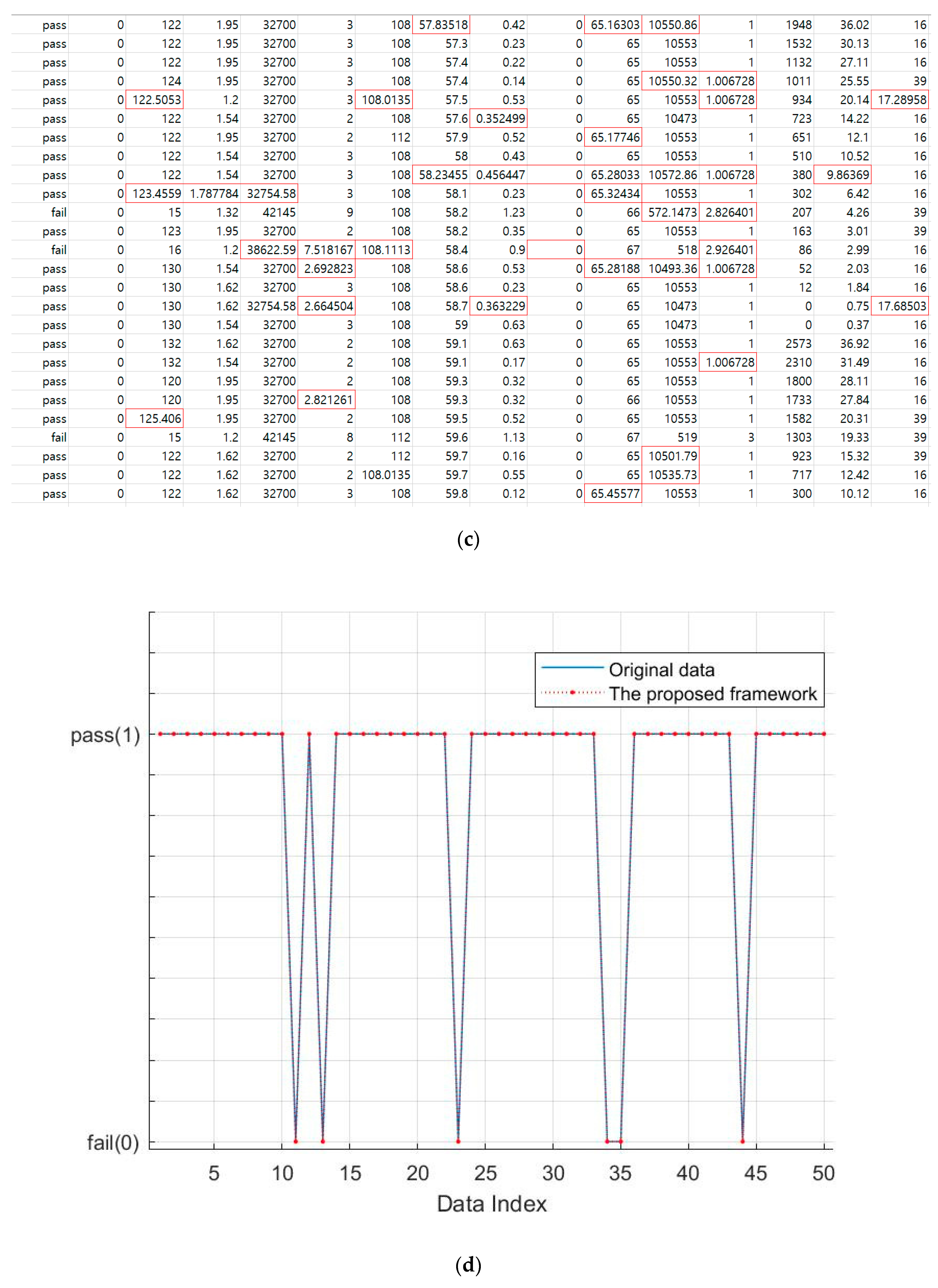
In order to show the effectiveness of the proposed framework, randomly generated data and their pass/fail outputs are considered. Figure 8a shows a data set from a randomized time series with Gaussian noise N ( 0 , 2 ) . The data set size is 50 data points and each data point is composed of 20 attributes. Their outputs are divided randomly into 44 passes (1) and 6 fails (0). Then, as shown in Figure 8b, several selected sections are considered as the sections with missing values.
Figure 8c shows a newly generated data set using the proposed framework. Finally, the pass/fail predictions using the randomly generated original data and the generated data are conducted as shown in Figure 8d.
The following section shows how the proposed framework is effective using the real data set.

4. Data Issues in Air Pressure System and Numerical Analysis

This section proves the effectiveness of the proposed framework and compares it with other existing methods. As discussed in previous sections, the proposed framework has the advantage of high performance in classification that comes from using accurate interpolations of missing values using the GPR-based GAN framework.
In order to show the effectiveness of the proposed framework, real-world data are used, specifically the APS failure Scania trucks data set [1]. The data consist of 170 attributes and 60,000 instance vectors. Training data are divided into 59,000 negative classes of APS-based faults and 1000 positive cases. Test data are divided into 15,625 negative cases and 375 positive cases. Several attributes in each piece of data have missing values. Table 4 shows the number of missing values in the APS data.
In order to estimate the missing values, the proposed framework is applied. Figure 9a shows the applied structure of the proposed framework. The generator regenerates the data by reflecting the discriminator’s objective value that distinguishes whether the data points generated by the generator are real data points or not. The deep neural network (DNN) is trained and tested to produce interpolated data, as shown in the red box in Figure 9b. A pass (1) or fail (0) is diagnosed using the DNN model. The DNN model has one input layer, multiple hidden layers, and one output layer. The hyperparameter for the experiment is set to 0.001 for its learning rate, 28 for the mini-batch size, 100 for max-epochs, and 0.5 for momentum.
In order to verify the effectiveness of the proposed framework, it is compared with other existing methods, including the classification and regression tree (CART), GPR, K-means, mean-based GAN, and compressed sensing (CS) methods. Table 5 summarizes these models and the relevant parameters.
Table 6 shows the results of the confusion matrix experiment with test data for each classification model.
As shown in Table 6 and Figure 10, the proposed GPR-based GAN framework shows the lowest rates of type-I and type-II errors.
Table 7 summarizes several performance evaluation indicators using the confusion matrix from Table 6. A true positive (TP) is given if a pass is indicated in real data and a pass is indicated by the classification model. A false negative (FN) is given if a pass is indicated in real data but a fail is indicated by the classification model. A false positive (FP) is given if a fail is indicated in real data but a pass is indicated by the classification model. A true negative (TN) is given if a fail is indicated in real data and a fail is indicated by the classification model.
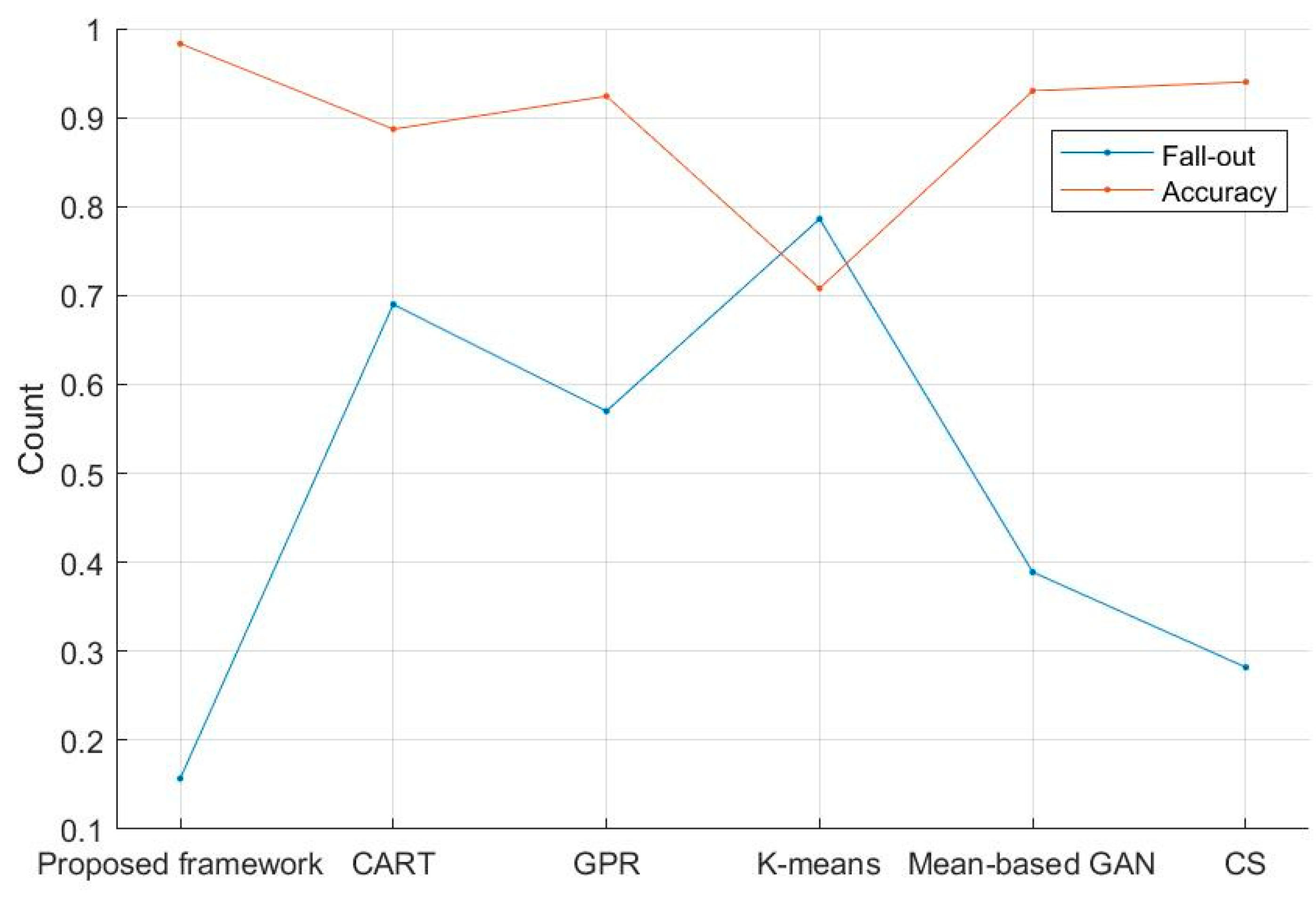
As outlined in Table 7, the definition of “precision” is the number of TP divided by the number of TP plus FP, while the “recall” is the number of TP divided by the number of TP plus FN. The “precision” and the “recall” handle the cases where the classification model classifies a pass when the real data indicates a pass. The “fall-out” is the number of FP divided by the number of TN plus FP. It handles misclassifications by the classification model when the real data indicate a fail but the classification model gives a pass. The “accuracy” is the number of TP plus TN divided by the sum of TP, TN, FP, and FN. “Accuracy” handles cases where both passes and fails are correctly classified. This is used as the main performance evaluation indicator.
As shown in Table 7 and Figure 11, the accuracy of the proposed framework is 98.3% and the fall-out is 15.7%, thus it is experimentally proved that the missing value handling using the proposed framework has better performance than other existing methods.

5. Conclusions

Failure analysis and relevant predictions generated from industrial big data are essential processes for industry in order to produce high quality and reliable products. However, most industrial big data sets are incomplete due to various issues. In these situations, existing algorithms fail to provide accurate corrections for the missing data. Therefore, any classification task executed on these kinds of incomplete data sets shows very poor performance.
In order to overcome this issue, the proposed framework generates a new complete data set using the proposed GPR-based GAN framework. The provided framework is based on the symmetry properties. First, the missing values are replaced with the mean value of the appropriate attribute. Then, the missing value estimates are refined by applying GPR. The data characteristics from this GPR process are linked to the GAN. Finally, the GAN is applied to generate further refinements to generate new data that are similar to the real data. The generated data are used as training data and help to overcome any data imbalances in the input data set.
In order to prove the performance of the proposed framework, it is compared with existing classification models using a real industrial data set related to APS failure in Scania trucks. Numerical analysis shows that the proposed framework has higher accuracy and lower fall-out than existing classification models. Through numerical analysis, it was confirmed that the proposed framework is effective compared with existing classification models.
The proposed framework can be used to estimate missing values in a data set with a high frequency of missing data. In addition, industrial data sets that are highly distorted with large data imbalances can be successfully analyzed using the proposed framework. In future studies, we hope to incorporate more efficient computation methods to handle data from multiple industrial areas.

Author Contributions

E.O. and H.L. conceptualized the framework and developed the methodologies. E.O. implemented and validated the framework. H.L. supervised the overall research processes. E.O. wrote the manuscript. H.L. reviewed and edited the manuscript. All authors have read and agreed to the published version of the manuscript.

Funding

This work was supported by Priority Research Centers Program through the National Research Foundation of Korea (NRF), funded by the Ministry of Education, Science, and Technology (2018R1A6A1A03024003).

Conflicts of Interest

The authors declare no conflict of interest.

References

  1. UCI Machine Learning Repository. 2017. Available online: https://archive.ics.uci.edu/ml/datasets/APS+Failure+at+Scania+Trucks (accessed on 8 December 2017).
  2. Paul, D.A. Missing Data; Sage Publications Inc.: Thousand Oaks, CA, USA, 2002; pp. 27–74. [Google Scholar]
  3. Dempster, P.; Laird, N.M.; Rubin, D.B. Maximum Likelihood from Incomplete Data via the EM Algorithm. J. R. Stat. Soc. 1997, 39, 1–22. [Google Scholar] [CrossRef]
  4. Moon, T.K. The expectation-maximization algorithm. IEEE Signal Process. Mag. 1996, 13, 47–60. [Google Scholar] [CrossRef]
  5. Hastie, T.; Tibshirani, R.; Sherlock, G.; Eisen, M.; Brown, P.; Bolstein, D. Imputing Missing Data for Gene Expression Arrays; Technical Report; Standford University Press: Standford, CA, USA, 1999. [Google Scholar]
  6. Troyanskaya, O.; Cantor, M.; Sherlock, G.; Brown, P.; Hastie, T.; Tibshirani, R.; Botstein, D.; Altman, R. Missing value estimation methods for DNA microarrays. Bioinformatics 2001, 17, 520–525. [Google Scholar] [CrossRef] [PubMed] [Green Version]
  7. Zhang, Z. Missing data imputation: Focusing on single imputation. Ann. Transl. Med. 2016, 4, 9. [Google Scholar] [CrossRef] [PubMed]
  8. Gondara, L.; Wang, K. Multiple imputation using deep denoising autoencoders. arXiv 2017, arXiv:1705.02737. [Google Scholar]
  9. Gemmeke, J.F.; Hamme, H.V.; Cranen, B.; Boves, L. Compressive Sensing for Missing Data Imputation in Noise Robust Speech Recognition. IEEE J. Sel. Top. Signal Process. 2010, 4, 272–287. [Google Scholar] [CrossRef] [Green Version]
  10. Oba, S.; Sato, M.; Takemasa, I.; Monden, M.; Matsubara, K.; Ishii, S. A Bayesian missing value estimation method for gene expression profile data. Bioinformatics 2003, 19, 2088–2096. [Google Scholar] [CrossRef]
  11. Little, R.J.; Rubin, D.B. Statistical Analysis with Missing Data, 3rd ed.; NJ John Wiley & Sons Inc.: Hoboken, NJ, USA, 2020; pp. 29–42. [Google Scholar]
  12. Gondek, C.; Hafner, D.; Sampson, O.R. Prediction of Failures in the Air Pressure System of Scania Trucks using a Random Forest and Feature Engineering. Adv. Intell. Data Anal. 2016, 9897, 398–402. [Google Scholar] [CrossRef]
  13. Perepu, S.K.; Tangirala, A.K. Reconstruction of missing data using compressed sensing techniques with adaptive dictionary. J. Process Control 2016, 47, 175–190. [Google Scholar] [CrossRef]
  14. Chodosh, N.; Wang, C.; Lucey, S. Deep Convolutional Compressed Sensing for LiDAR Depth Completion. Comput. Vis. ACCV 2018, 11361, 499–513. [Google Scholar] [CrossRef] [Green Version]
  15. Williams, C.K.I.; Rasmussen, C.E. Gaussian Processes for Machine Learning; The MIT Press: London, UK, 2006; pp. 7–128. [Google Scholar]
  16. Williams, C.K.I.; Rasmussen, C.E. Gaussian Processes for Regression. Adv. Neural Process. Syst. 1996, 8, 514–520. [Google Scholar]
  17. Rasmussen, C.E. Gaussian Processes in Machine Learning. Adv. Lect. Mach. Learn. 2004, 3176, 63–71. [Google Scholar] [CrossRef] [Green Version]
  18. Chu, W.; Ghahramani, Z. Gaussian Processes for Ordinal Regression. J. Mach. Learn. Res. 2005, 6, 1019–1041. [Google Scholar]
  19. Schulz, E.; Speekenbrink, M.; Krause, A. A tutorial on Gaussian process regression: Modelling, exploring, and exploiting functions. J. Math. Psychol. 2017, 85, 1–16. [Google Scholar] [CrossRef]
  20. Jochem, V.; Juan, P.R.; Anatoly, G.; Jesus, D.; Jose, M.; Gustau, C. Spectral band selection for vegetation properties retrieval using Gaussian processes regression. Int. J. Appl. Earth Obs. Geoinf. 2016, 52, 554–567. [Google Scholar] [CrossRef]
  21. Ak, C.; Ergonul, O.; Sencan, I.; Torunoglu, M.A.; Gonen, M. Spatiotemporal prediction of infectious diseases using structured Gaussian processes with application to Crimean-Congo hemorrhagic fever. PLoS Negl. Trop. Dis. 2018, 12, e0006737. [Google Scholar] [CrossRef] [PubMed] [Green Version]
  22. Luttinen, J.; Ilin, A. Efficient Gaussian process inference for short-scale spatio-temporal modeling. In Proceedings of the 15th International Conference on Artificial Intelligence and Statistics, La Palma, Canary Islands, 21–23 April 2012; pp. 741–750. [Google Scholar]
  23. Nguyen, D.; Peters, J. Learning Robot Dynamics for Computed Torque Control using Local Gaussian Processes Regression. In Proceedings of the ECSIS Symposium on Learning and Adaptive Behaviors for Robotic Systems, Edinburgh, UK, 6–8 August 2008; pp. 59–64. [Google Scholar]
  24. Nguyen, L.; Hu, G.; Spanos, C.J. Spatio-temporal environmental monitoring for smart buildings. In Proceedings of the 13th IEEE International Conference on Control and Automation, Ohrid, Macedonia, 3–6 July 2017; pp. 277–282. [Google Scholar]
  25. Chen, N.; Qian, Z.; Meng, X.; Nabney, I.T. Short-term wind power forecasting using Gaussian processes. In Proceedings of the 23rd International Joint Conference on Artificial Intelligence, Beijing, China, 3–9 August 2013; pp. 2790–2796. [Google Scholar]
  26. Oh, E.; Lee, H. Development of a Convolution-Based Multi-Directional and Parallel Ant Colony Algorithm Considering a Network with Dynamic Topology Changes. Appl. Sci. 2019, 9, 3646. [Google Scholar] [CrossRef] [Green Version]
  27. Goodfellow, I.J.; Pouget, J.; Mirza, M.; Xu, B.; WardeFarley, D.; Ozair, S.; Courville, A.; Bengio, Y. Generative Adversarial Nets. In Proceedings of the NIPS 2014, Montreal, QC, Canada, 8–13 December 2014; pp. 1–9. [Google Scholar]
  28. Kim, H.; Lee, H. Fault Detect and Classification Framework for Semiconductor Manufacturing Processes using Missing Data Estimation and Generative Adversary Network. J. Korean Inst. Intell. Syst. 2018, 28, 393–400. [Google Scholar] [CrossRef]
  29. Yoon, J.; Jordon, J.; Schaar, M. GAIN: Missing Data Imputation using Generative Adversarial Nets. arXiv 2018, arXiv:1806.02920. [Google Scholar]
  30. Kim, H.; Lee, H. Generative Adversarial Networks based Data Generation Framework for Overcoming Imbalanced Manufacturing Process Data. J. Korean Inst. Intell. Syst. 2019, 29, 1–8. [Google Scholar] [CrossRef]
  31. Shang, C.; Palmer, A.; Sun, J.; Chen, K.; Lu, J.; Bi, J. VIGAN: Missing view imputation with generative adversarial networks. In Proceedings of the IEEE International Conference on Big Data, Boston, MA, USA, 11–14 December 2017; pp. 766–775. [Google Scholar]
  32. Mao, X.; Li, Q.; Xie, H.; Lau, R.Y.K.; Wang, Z.; Smolley, S.P. Least Squares Generative Adversarial Networks. In Proceedings of the IEEE International Conference on Computer Vision (ICCV), Venice, Italy, 22–29 October 2017; pp. 2794–2802. [Google Scholar]
  33. Zhao, J.; Mathieu, M.; LeCun, Y. Energy-based generative adversarial network. arXiv 2016, arXiv:1609.03126. [Google Scholar]
  34. Li, J.; Liang, X.; Wei, Y.; Xu, T.; Feng, J.; Yan, S. Perceptual Generative Adversarial Networks for Small Object Detection. In Proceedings of the IEEE Conference on Computer Vision and Pattern Recognition (CVPR), Hawaii, HI, USA, 21–26 July 2017; pp. 1222–1230. [Google Scholar]
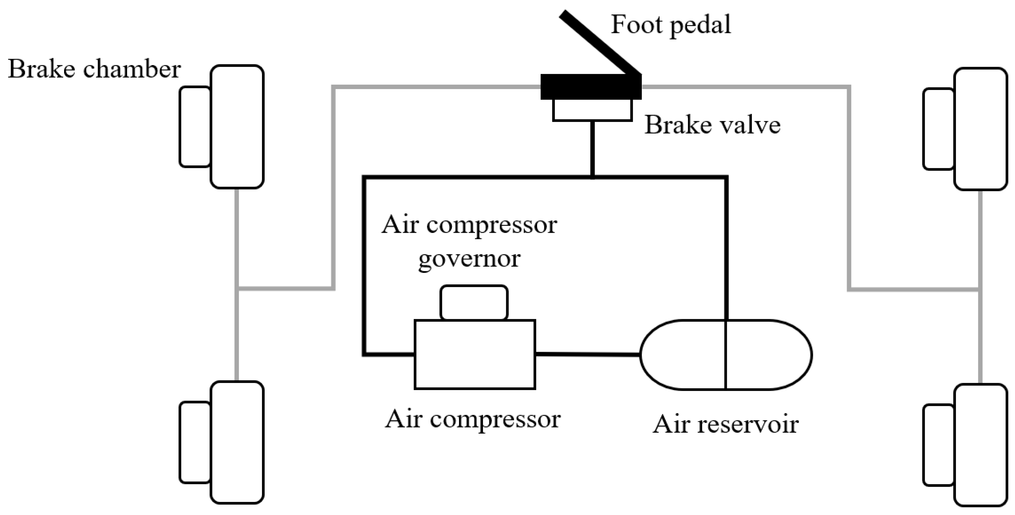
Figure 1. Air pressure system (APS) structure.
Symmetry 12 00669 g001
Figure 2. Issues from missing values in APS data for Scania trucks.
Symmetry 12 00669 g002
Figure 3. Graphical model of Gaussian process regression.
Symmetry 12 00669 g003
Figure 4. General architecture of generative adversarial network.
Symmetry 12 00669 g004
Figure 5. Missing value estimation and data generation procedures using the proposed framework.
Symmetry 12 00669 g005
Figure 6. Backpropagation-based learning process for the ggenerative adversarial network (GAN). (a) architecture of the discriminator from real data; (b) architecture of the discriminator from fake data; (c) architecture of the generator.
Symmetry 12 00669 g006aSymmetry 12 00669 g006b
Figure 7. A time series-based numerical analysis using GPR-GAN: (a) randomly generated original data; (b) comparison between actual data and data estimated using GPR.
Symmetry 12 00669 g007aSymmetry 12 00669 g007b
Figure 8. Numerical analysis using the proposed framework: (a) randomly generated data and their pass/fail outputs; (b) randomly selected missing values in the data set; (c) newly generated data using the proposed framework; (d) classification results between the original data and the generated data using the proposed framework.
Symmetry 12 00669 g008aSymmetry 12 00669 g008b
Figure 9. GAN-based DNN structure: (a) structure of the proposed framework; (b) classification structure using DNN.
Symmetry 12 00669 g009
Figure 10. Comparison graphs among each classification model: (a) comparisons of “an actual passes versus predicted passes” in the negative class; (b) comparison of “an actual failures versus predicted failures” in the positive class.
Symmetry 12 00669 g010
Figure 11. Comparison graph of “fall-out” and “accuracy” among four test models.
Symmetry 12 00669 g011
Table 1. Existing research studies and applications for estimating missing data.
Missing Value Handling MethodResearch Studies and ApplicationsMain Estimation Techniques and Frameworks
ImputationPaul [2]Multiple imputation (MI)-based missing value estimation
Dempster, Laird, and Rubin [3]Probability modeling maximum likelihood estimation (MLE)-based estimation
Expectation maximization-based estimation [4]
Hastie et al. [5],
Troyanskaya et al. [6]
Singular value decomposition (SVD) and K-nearest neighbor (KNN)-based missing data imputation
Zhang [7]Regression-based imputation
Gondara and Wang [8]Deep denoising autoencoder-based imputation
Gemmeke et al. [9]Missing data imputation using sparse imputation-based compressive sensing (CS)
EstimationOba et al. [10]Bayesian network-based preprocessing
Gene profiling expression
Little and Rubin [11]Least squares-based missing data analysis
Gondek, Hafner, and Sampson [12]Missing value imputation using random forest and feature engineering
Perepu and Tangirala [13]Missing value estimation using a CS method with adaptive dictionary
Chodosh, Wang, and Lucey [14]Estimating a dense depth map using a CS method and alternating direction neural networks
Table 2. Research studies and applications using Gaussian processes regression (GPR).
Research Studies Using GPRApplication Areas
Jochem et al. [20]Automated spectral band analysis
Ak et al. [21]The time and space prediction of an infectious diseases
Luttinen and Ilin [22]Sea level temperature reconstruction using GPR
Nguyen and Peters [23]Kinetics model estimation
Nguyen, Hu and Spanos [24]Efficient building field formation using an estimation of indoor environment fields
Chen et al. [25]Wind prediction for energy efficiency
Oh and Lee [26]Estimation of pheromone values based on ant colony optimization
Table 3. Research studies and applications using a generative adversarial network (GAN).
Research Studies Using GANApplication and Characteristics
Kim and Lee [28]Missing data generation of semiconductor manufacturing processes data
method: Oversample → GAN based data generation
Yoon, Jordon, and Schaar [29]Missing data imputation of breast cancer, spam, letter recognition, credit, news data
GAN-based hint generation
Kim and Lee [30]Missing data generation of steel Plates faults data
Estimate the missing value by adding missing term based on the GAN
Shang et al. [31]Image generation
GAN-based missing view imputation
Mao et al. [32]Image generation
Least squares loss function-based discriminator in a GAN
Zhao, Mathieu, and Le Cun [33]Image generation
Energy value allocation according to data density-based a discriminator in a GAN
Li et al. [34]Object detection
GAN-based high-quality image generation
Table 4. Missing data issues in APS data.
CategoriesTotal SizeData Item with Missing ValuesPercentages of Missing Items
Training dataNumber of attributes170170100%
Data set60,00059,99899.99%
Test dataNumber of attributes17016999.41%
Data set16,00016,000100%
Table 5. Models and parameters for each testing algorithm. Note: classification and regression tree = CART; compressed sensing = CS.
Tested FrameworksEquationParameter
GPR-based GAN
(Proposed framework)
min G   max D V ( D , G ) = E x ~ p d a t a ( x ) [ log D ( x ) ] + E z ~ p z ( z ) [ log ( 1 D ( G ( z ) ) ) ] Max epochs = 100
Learning rate = 0.1
Momentum = 0.5
CART I G ( f ) = 1 i = 1 m f i 2
C o s t   f u n c t i o n = m l e f t m I G ( f l e f t ) + m r i g h t m I G ( f r i g h t )
Tree’s depth = 50,000
Costs of misclassification = 1:1
Occupation percentage = 1:1
GPR f ~ GP ( m ( x ) , k ( x , x * ) ) Nonparametric
K-means arg   min S i = 1 k x S i x μ i 2 Maximum number of runs = 100
Distance calculation method = Euclidean
Surface pretreatment = Normalization
Mean-based GAN min G   max D V ( D , G ) = E x ~ p d a t a ( x ) [ log D ( x ) ] + E z ~ p z ( z ) [ log ( 1 D ( G ( z ) ) ) ] Max epochs = 100
Learning rate = 0.1
Momentum = 0.5
CS min x x 1   s u b j e c t   t o   y = w x Max epochs = 100
Learning rate = 0.1
Table 6. Confusion matrix for each classification model.
Proposed Framework Pass (Predicted)Fail (Predicted)
Pass (Actual)15,418207
Fail (Actual)59316
CART Pass (Predicted)Fail (Predicted)
Pass (Actual)14,0841541
Fail (Actual)259116
GPR Pass (Predicted)Fail (Predicted)
Pass (Actual)14,6251000
Fail (Actual)214161
K-means Pass (Predicted)Fail (Predicted)
Pass (Actual)11,2494376
Fail (Actual)29580
Mean-based GAN Pass (Predicted)Fail (Predicted)
Pass (Actual)14,654971
Fail (Actual)146229
CS Pass (Predicted)Fail (Predicted)
Pass (Actual)14,782843
Fail (Actual)106269
Table 7. Performance evaluation indicators.
Proposed FrameworkCARTGPRK-MeansMean-Based GANCS
Precision0.9960.9810.9850.9740.990.992
Recall0.9860.9010.9360.7190.9370.946
Fall-out0.1570.6900.5700.7860.3890.282
Accuracy0.9830.8870.9240.7080.930.94