Unsupervised Clustering for Hyperspectral Images


Abstract
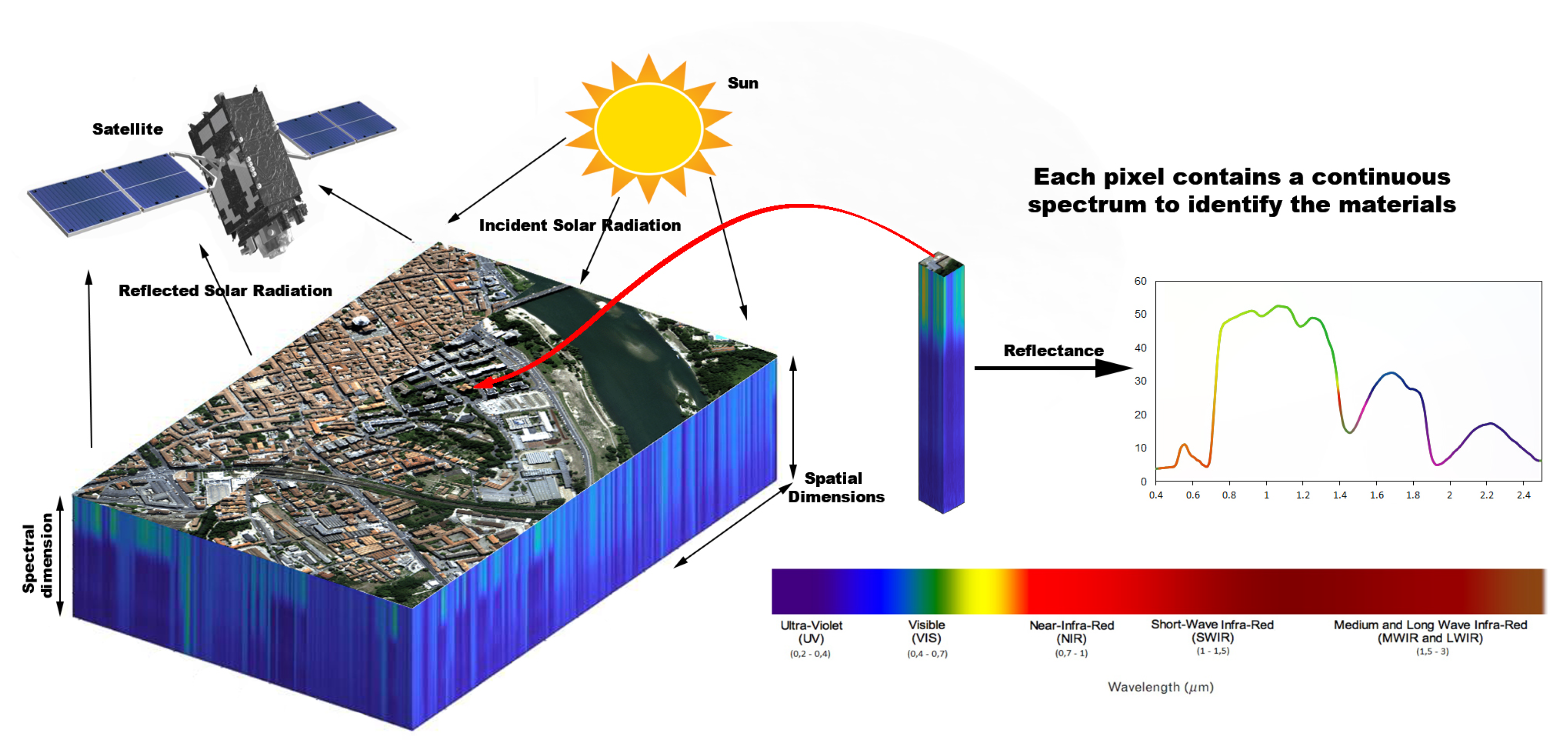
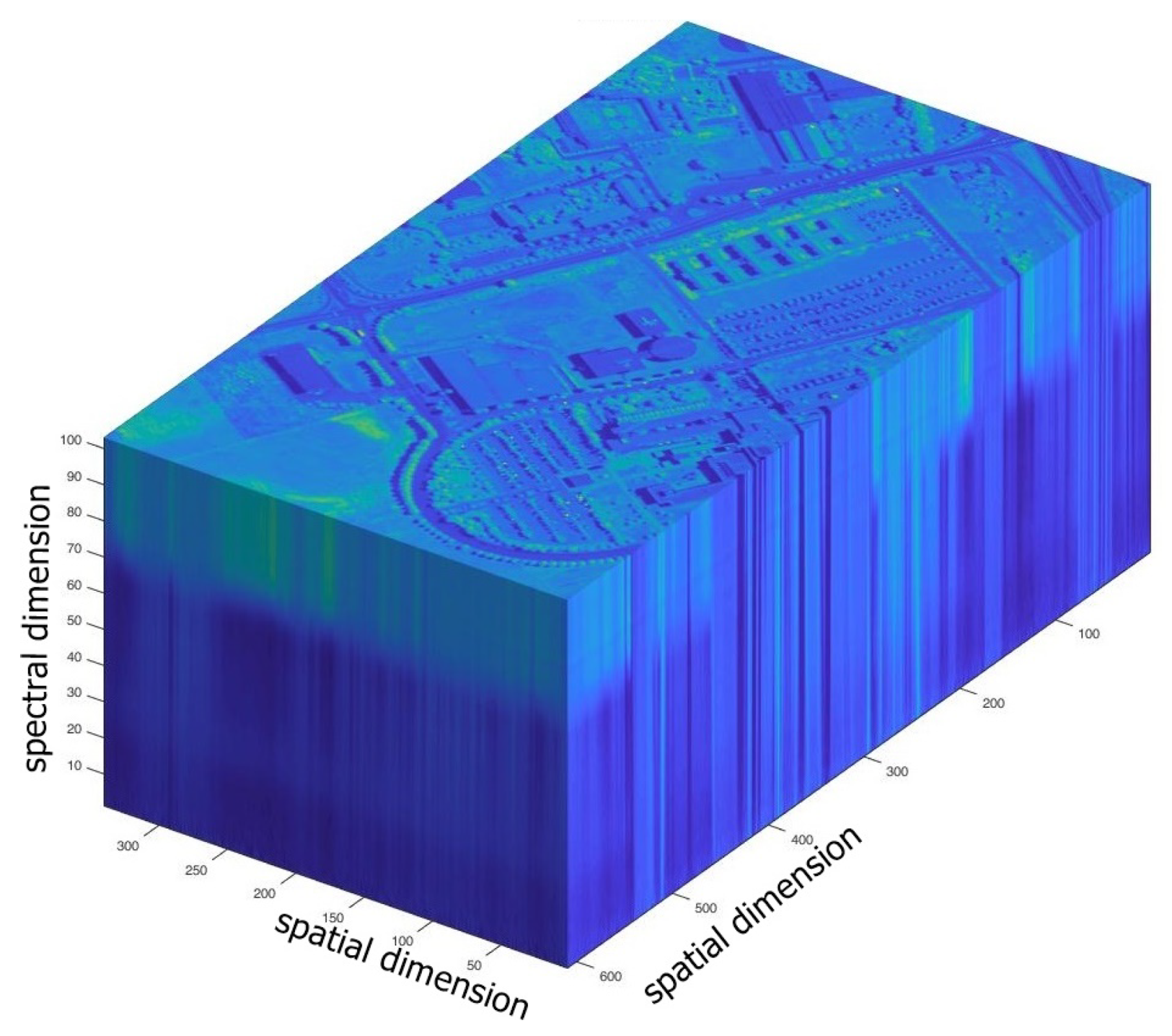
1. Introduction
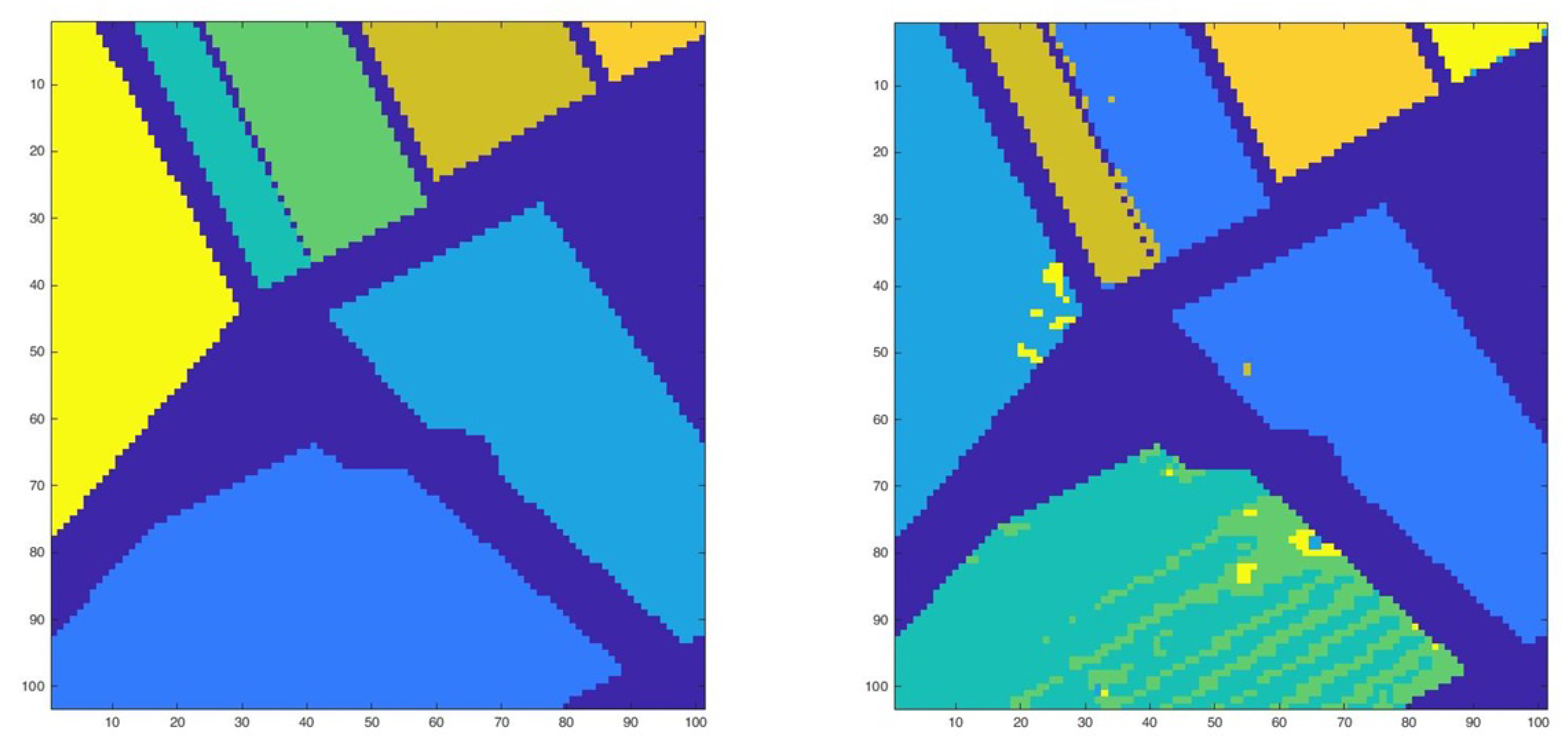
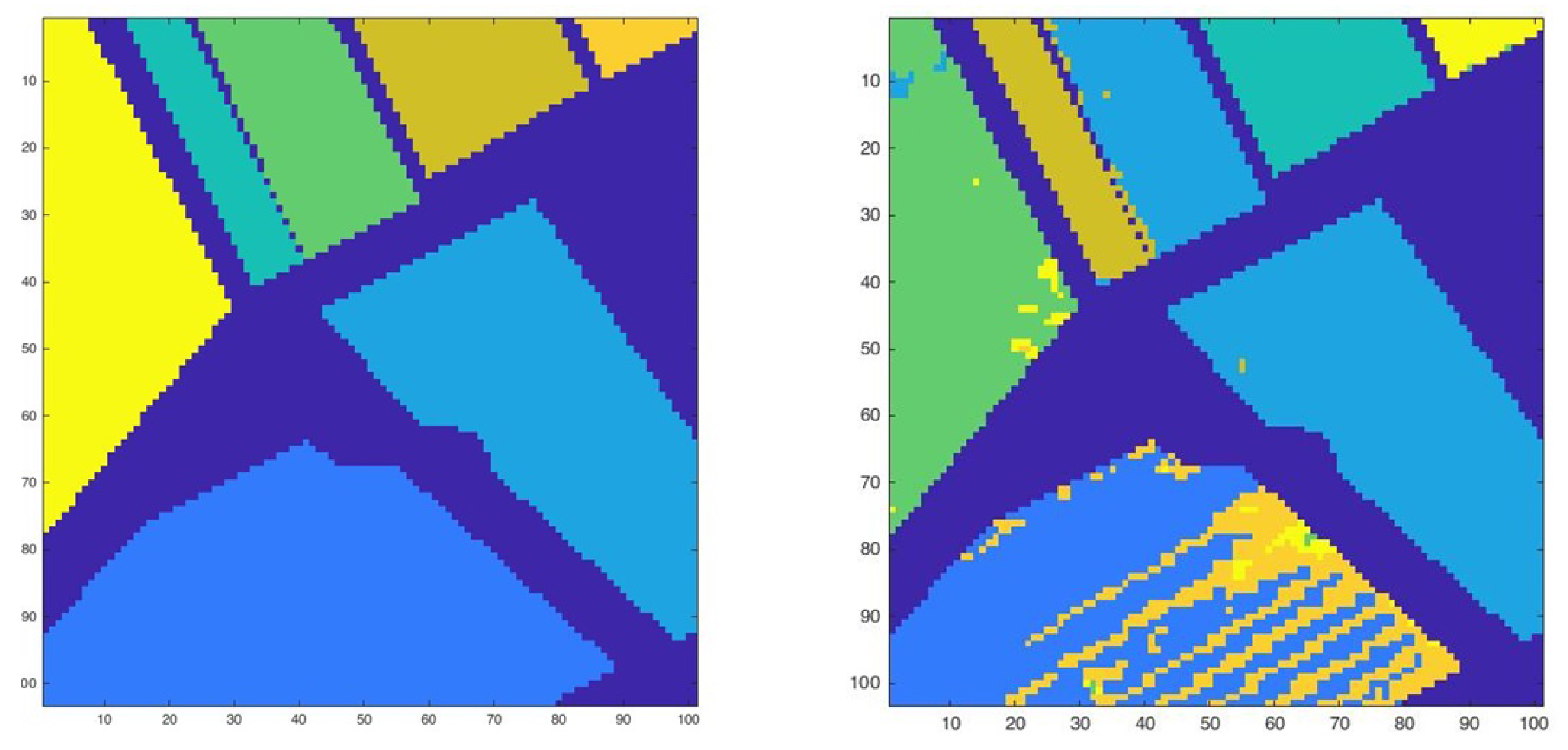
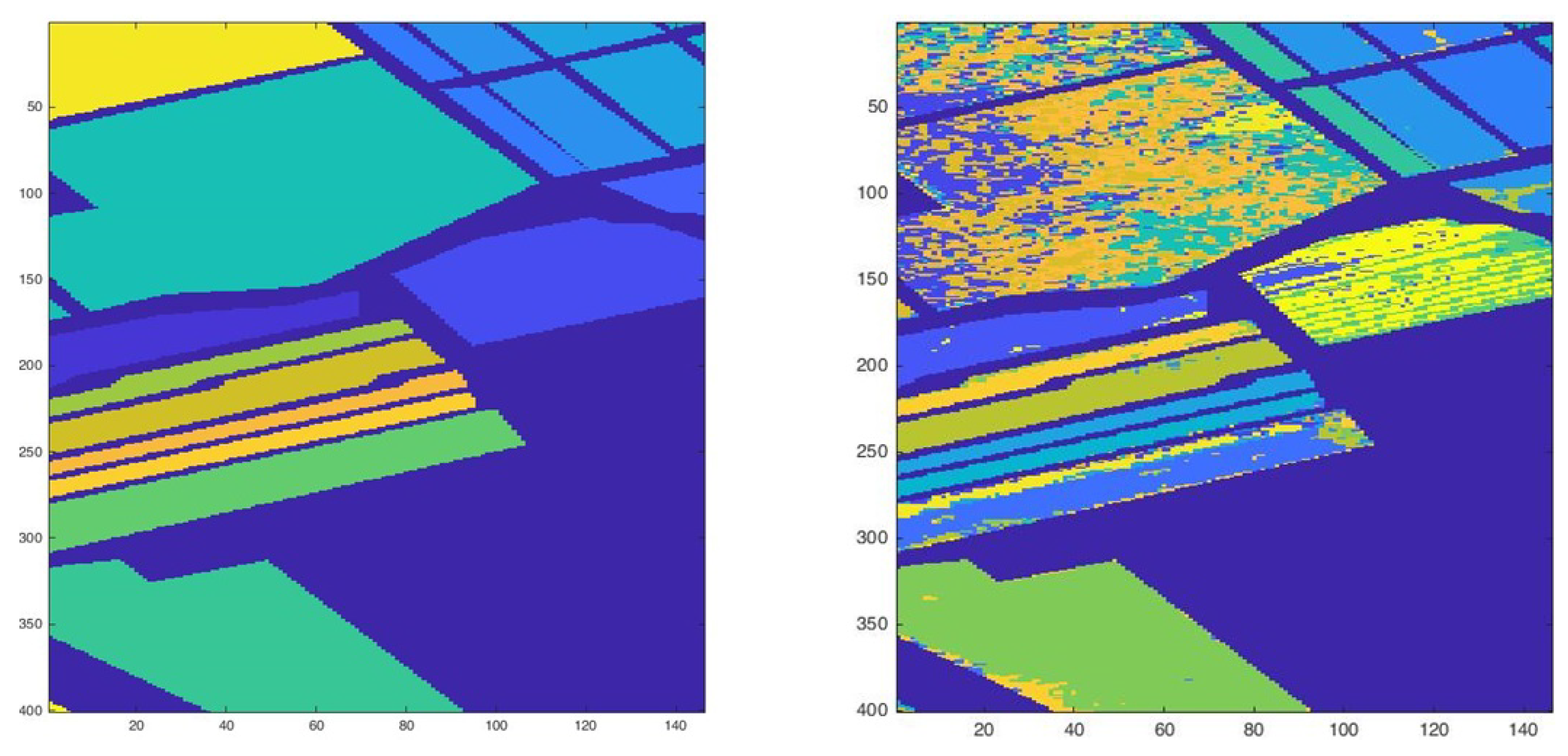
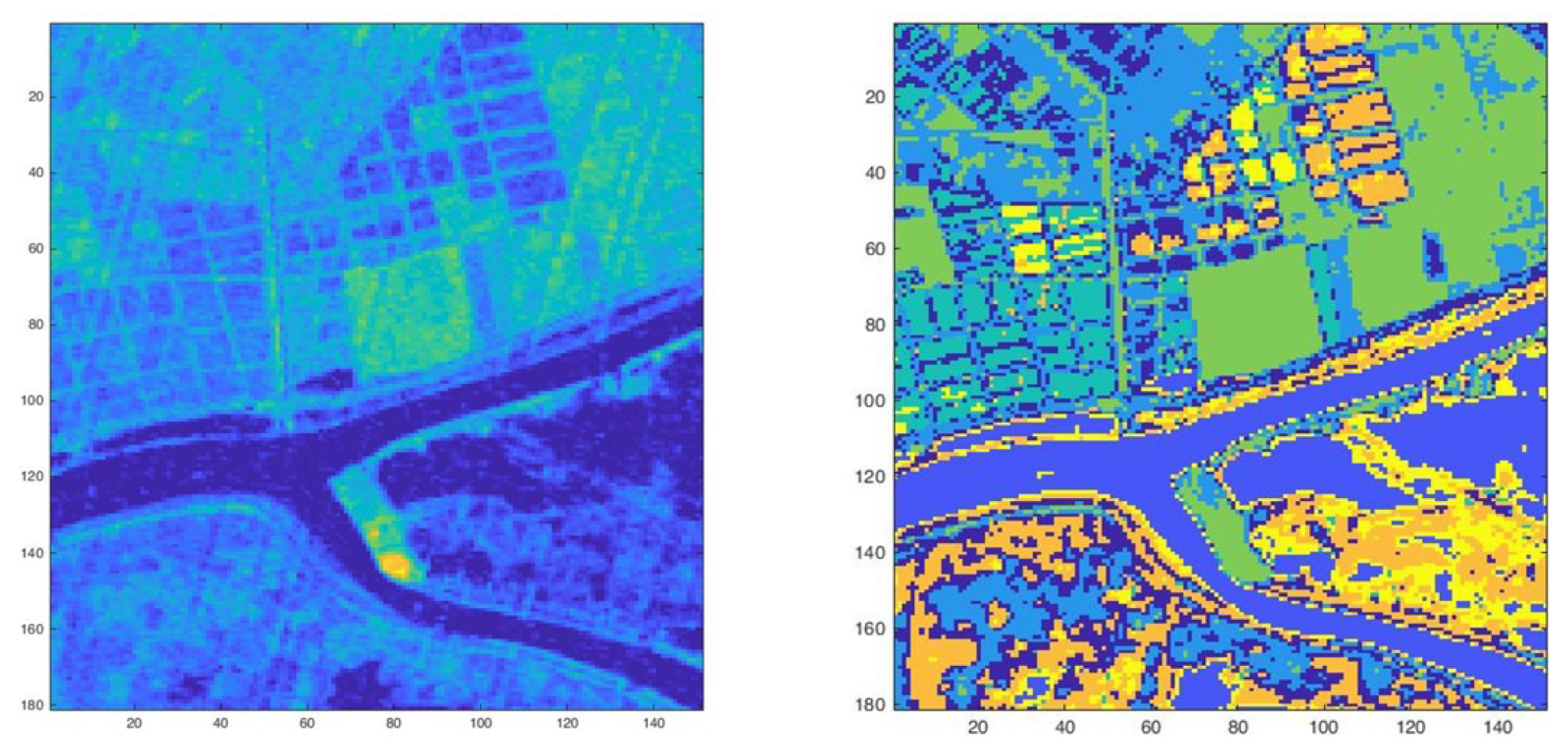
2. Results of Unsupervised Clustering
2.1. Hierarchical Clustering
2.2. K-Means Clustering
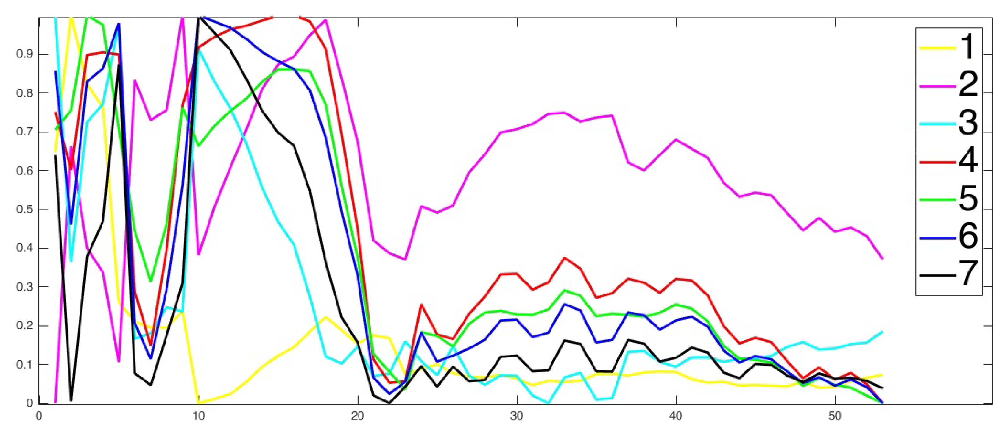
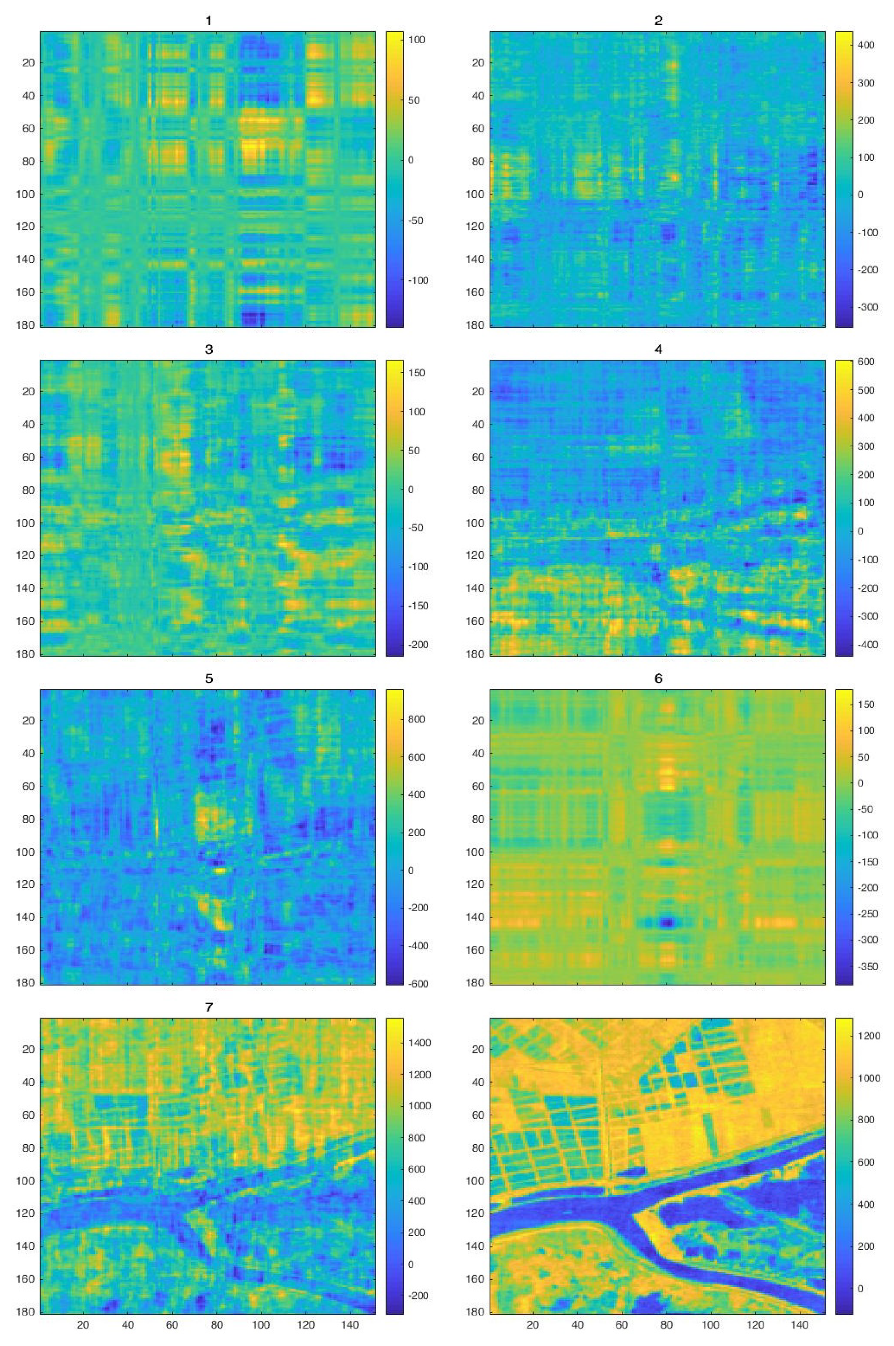
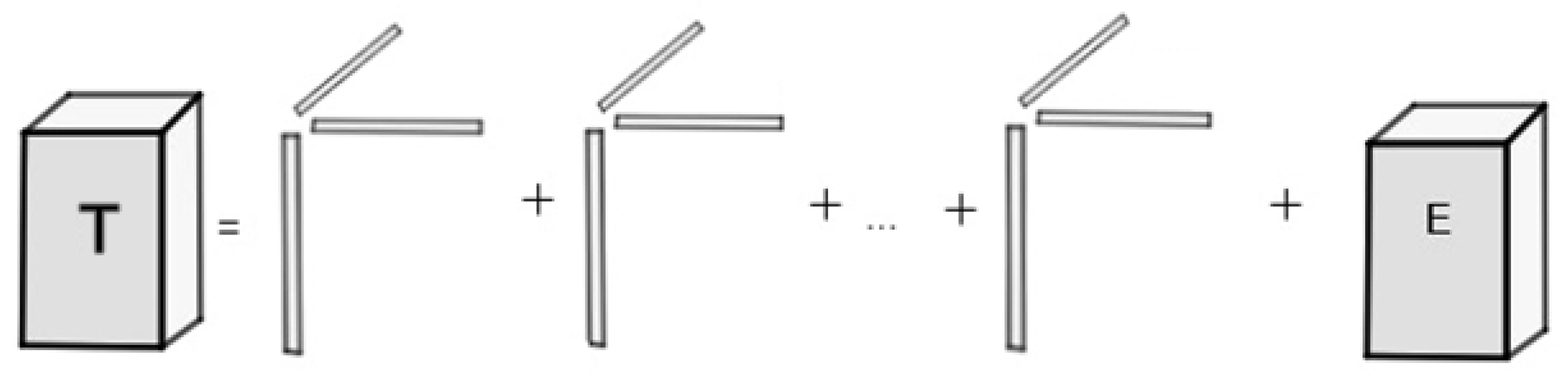
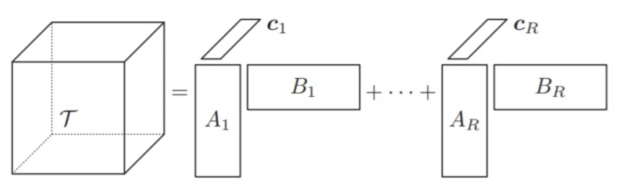
2.3. Parafac Classification
| Algorithm 1: The construction of abundance map |
 |
3. Discussion
4. Methods
4.1. Parafac Decomposition
4.2. K-means and Hierarchical Clustering
5. Conclusions
Author Contributions
Funding
Conflicts of Interest
References
- Audebert, N.; Saux, B.; Lefèvre, S. Deep Learning for Classification of Hyperspectral Data: A Comparative Review. IEEE Geosci. Remote Sens. Mag. 2019, 7. [Google Scholar] [CrossRef]
- Wang, D.; Cheng, B. An Unsupervised Classification Method of Remote Sensing Images Based on Ant Colony Optimization Algorithm. In Advanced Data Mining and Applications; Cao, L., Feng, Y., Zhong, J., Eds.; Springer: Berlin/Heidelberg, Germany, 2010; pp. 294–301. [Google Scholar]
- Wu, M.; Wei, D.Z.L.Z.Y. Hyperspectral Face Recognition with Patch-Based Low Rank Tensor Decomposition and PFFT Algorithm. Symmetry 2018, 10, 714. [Google Scholar] [CrossRef]
- Ganci, G.; Vicari, A.; Fortuna, L.; Negro, C.D. The HOTSAT volcano monitoring system based on combined use of SEVIRI and MODIS multispectral data. Ann. Geophys. 2011, 54. [Google Scholar] [CrossRef]
- Zhou, D.; Xiao, J.; Bonafoni, S.; Berger, C.; Deilami, K.; Zhou, Y.; Frolking, S.; Yao, R.; Qiao, Z.; Sobrino, J. Satellite Remote Sensing of Surface Urban Heat Islands: Progress, Challenges, and Perspectives. Remote Sens. 2018, 11, 48. [Google Scholar] [CrossRef]
- Sahar, A. Hyperspectral Image Classification Using Unsupervised Algorithms. Int. J. Adv. Comput. Sci. Appl. 2016, 7. [Google Scholar] [CrossRef]
- Moughal, T.A. Hyperspectral image classification using Support Vector Machine. J. Phys. Conf. Ser. 2013, 439, 012042. [Google Scholar] [CrossRef]
- Hosseini, L.; Kandovan, R. Hyperspectral Image Classification Based on Hierarchical SVM Algorithm for Improving Overall Accuracy. Adv. Remote Sens. 2017, 6, 66–75. [Google Scholar] [CrossRef]
- Senapati, S. Unsupervised Classification of Hyperspectral Images Based on Spectral Features. Bacherlor’s Thesis, Department of Electronics and Communication Engineering, National Institute of Technology Rourkela, Rourkela, India, 2015. [Google Scholar]
- Ranjan, S.; Nayak, D.; Kumar, S.; Dash, R.; Majhi, B. Hyperspectral image classification: A k-means clustering based approach. In Proceedings of the 2017 4th International Conference on Advanced Computing and Communication Systems (ICACCS) 2017, Coimbatore, India, 6–7 January 2017; pp. 1–7. [Google Scholar] [CrossRef]
- Veganzones, M.A.; Cohen, J.; Farias, R.C.; Marrero, R.; Chanussot, J.; Comon, P. Multilinear spectral unmixing of hyperspectral multiangle images. In Proceedings of the 2015 23rd European Signal Processing Conference (EUSIPCO), Nice, France, 31 August –4 September 2015; pp. 744–748. [Google Scholar]
- Phan, A.H.; Cichocki, A. Tensor decompositions for feature extraction and classification of high dimensional datasets. Nonlinear Theory Its Appl. IEICE 2010, 1, 37–68. [Google Scholar] [CrossRef]
- Arena, P.; Bucolo, M.; Fazzino, S.; Fortuna, L.; Frasca, M. The CNN Paradigm: Shapes and Complexity. Int. J. Bifurc. Chaos 2005, 15, 2063–2090. [Google Scholar] [CrossRef]
- GIC. Grupo de Inteligencia Computacional Hyperspectral Remote Sensing Scenes. Available online: http://www.ehu.eus/ (accessed on 1 September 2019).
- USGS. Earthexplorer.usgs.gov, U.S. Geological Survey. Available online: https://earthexplorer.usgs.gov (accessed on 1 September 2019).
- Christian, E.; Jiman, H.; Kim-Kwang, C. Pervasive Systems, Algorithms and Networks. In Proceedings of the 16th International Symposium (I-SPAN 2019), Naples, Italy, 16–20 September 2019. [Google Scholar] [CrossRef]
- GeeksforGeeks. A Computer Science Portal for Geeks, GeeksforGeeks. Available online: https://www.geeksforgeeks.org/ (accessed on 1 September 2019).
- Tamara Kolda, B.W. Tensor Decompositions and Applications. Soc. Ind. Appl. Math. 2009, 51, 455–500. [Google Scholar]
- Ignat Domanov, L.L. On the uniqueness of the canonical polyadic decomposition of third-order tensors-Part II: Uniqueness of the overall decomposition. SIAM J. Matrix Anal. Appl. 2013, 34, 876–903. [Google Scholar]
- Chen Shi, L.W. Linear Spatial Spectral Mixture Model. IEEE Trans. Geosci. Remote. Sens. 2016, 54, 3599–3611. [Google Scholar]
- Yuntao, Q.; Fengchao, X. Matrix-Vector Nonnegative Tensor Factorization for Blind Unmixing of Hyperspectral Imagery. IEEE Trans. Geosci. Remote Sens. 2017, 55, 1776–1792. [Google Scholar]
- Sorber, L.; Barel, M.V.; Lathauwer, L.D. Optimization-Based Algorithms for Tensor Decompositions: Canonical Polyadic Decomposition, Decomposition in Rank-(Lr,Lr,1) Terms And A New Generalization. SIAM J. Optim. 2013, 23, 695–720. [Google Scholar] [CrossRef]
- Veganzones, M.; Cohen, J. Canonical Polyadic Decomposition of Hyperspectral Patch Tensors. In Proceedings of the 2016 24th European Signal Processing Conference (EUSIPCO), Budapest, Hungary, 28 August–2 September 2016; pp. 2176–2180. [Google Scholar] [CrossRef]
- Nielsen, F. Hierarchical Clustering. In Introduction to HPC with MPI for Data Science; Springer: Berlin, Germany, 2016; pp. 195–211. ISBN 978-3-319-21902-8. [Google Scholar] [CrossRef]
- Scikit-Learn. Scikit-learn, Learn: Machine Learning in Python—Scikit-Learn 0.16.1 Documentation. Available online: https://scikit-learn.org/ (accessed on 1 November 2019).
- Doan, T.; Kalita, J. Predicting run time of classification algorithms using meta-learning. Int. J. Mach. Learn. Cybern. 2016, 8. [Google Scholar] [CrossRef]
- Bilius, L.B.; Pentiuc, S.G.; Brie, D.; Miron, S. Analysis of hyperspectral images using supervised learning techniques. In Proceedings of the 23rd International Conference on System Theory, Control and Computing, ICSTCC, Sinaia, Romania, 9–11 October 2019. [Google Scholar] [CrossRef]


| 1 | 2 | 3 | 4 | 5 | 6 | 7 | Total | |
|---|---|---|---|---|---|---|---|---|
| 1 | 2291 | 0 | 0 | 0 | 0 | 29 | 6 | 2326 |
| 2 | 0 | 1772 | 2 | 0 | 0 | 0 | 0 | 1774 |
| 3 | 0 | 2 | 362 | 0 | 0 | 0 | 0 | 364 |
| 4 | 0 | 657 | 25 | 0 | 0 | 0 | 0 | 682 |
| 5 | 0 | 0 | 0 | 0 | 539 | 0 | 0 | 539 |
| 6 | 0 | 0 | 0 | 0 | 0 | 98 | 4 | 102 |
| 7 | 0 | 0 | 0 | 0 | 0 | 24 | 1258 | 1282 |
| % | 98.49 | 99.88 | 99.45 | 0 | 100 | 96.07 | 98.12 |
| 1 | 2 | 3 | 4 | 5 | 6 | 7 | Total | |
|---|---|---|---|---|---|---|---|---|
| 1 | 2280 | 0 | 0 | 0 | 0 | 41 | 5 | 2326 |
| 2 | 0 | 1772 | 2 | 0 | 0 | 0 | 0 | 1774 |
| 3 | 0 | 2 | 362 | 0 | 0 | 0 | 0 | 364 |
| 4 | 0 | 656 | 26 | 0 | 0 | 0 | 0 | 682 |
| 5 | 0 | 1 | 0 | 0 | 538 | 0 | 0 | 539 |
| 6 | 0 | 0 | 0 | 0 | 0 | 100 | 2 | 102 |
| 7 | 2 | 16 | 0 | 0 | 0 | 29 | 1235 | 1282 |
| % | 98.02 | 99.88 | 99.45 | 0 | 99.81 | 98.03 | 96.33 |
| Set | Sil. Score 1 | DB 2 | Exe. 3 | Acc. 4 | Cl. 5 |
|---|---|---|---|---|---|
| 1 | 0.701(7) | 0.400 | 0.020 | 0.894 | 7 |
| 2 | 0.427(16) | 0.731 | 0.094 | 0.847 | 16 |
| 3 | 0.539(11) | 0.586 | 0.012 | 0.961 | 6 |
| 4 | 0.802 (6) | 0.568 | 0.027 | 0.946 | 6 |
| 5 | 0.260 (7) | 1.288 | 0.058 | - | - |
| Set | Sil. Score 1 | DB 2 | Exe. 3 | Acc. 4 | Cl. 5 |
|---|---|---|---|---|---|
| 1 | 0.700(7) | 0.411 | 1.925 | 0.889 | 7 |
| 2 | 0.4462(17) | 0.711 | 19.963 | 0.847 | 16 |
| 3 | 0.575(10) | 0.520 | 0.707 | 0.969 | 6 |
| 4 | 0.806(6) | 0.550 | 0.877 | 0.950 | 6 |
| 5 | 0.309(7) | 1.154 | 3.854 | - | - |
| Set | 1 | 2 | 3 | 4 | 5 |
|---|---|---|---|---|---|
| Execution Time | |||||
| Parafac 1 | 4.23 | 12.03 | 3.63 | 4.27 | 3.25 |
| Classification 2 | 5975 | 2880 | 2363 | 3603 | 1498 |
| Class. K-means 3 | 0.030 | 36.47 | 0.048 | 0.069 | 0.059 |
| Class. Hierarchical 4 | 2.448 | 3794 | 3.954 | 5.290 | 3.855 |
| Class | Class Distribution | ||||
| 1 | 6 | 14 | 4 | 5 | - |
| 2 | 5 | 5 | 3 | 2 | - |
| 3 | 6 | 16 | 4 | 1 | - |
| 4 | 4 | 5 | 1 | 2 | - |
| 5 | 7 | 1 | 3 | 2 | - |
| 6 | 6 | 8 | 5 | 3 | - |
| 7 | 4 | 14 | - | - | - |
| 8 | - | 1 | - | - | - |
| 9 | - | 7 | - | - | - |
| 10 | - | 16 | - | - | - |
| 11 | - | 5 | - | - | - |
| 12 | - | 6 | - | - | - |
| 13 | - | 16 | - | - | - |
| 14 | - | 9 | - | - | - |
| 15 | - | 7 | - | - | - |
| 16 | - | 14 | - | - | - |
© 2020 by the authors. Licensee MDPI, Basel, Switzerland. This article is an open access article distributed under the terms and conditions of the Creative Commons Attribution (CC BY) license (http://creativecommons.org/licenses/by/4.0/).
Share and Cite
Bilius, L.B.; Pentiuc, S.G. Unsupervised Clustering for Hyperspectral Images. Symmetry 2020, 12, 277. https://doi.org/10.3390/sym12020277
Bilius LB, Pentiuc SG. Unsupervised Clustering for Hyperspectral Images. Symmetry. 2020; 12(2):277. https://doi.org/10.3390/sym12020277
Chicago/Turabian StyleBilius, Laura Bianca, and Stefan Gheorghe Pentiuc. 2020. "Unsupervised Clustering for Hyperspectral Images" Symmetry 12, no. 2: 277. https://doi.org/10.3390/sym12020277
APA StyleBilius, L. B., & Pentiuc, S. G. (2020). Unsupervised Clustering for Hyperspectral Images. Symmetry, 12(2), 277. https://doi.org/10.3390/sym12020277