Distribution Function, Probability Generating Function and Archimedean Generator

Abstract

Archimedean copulas form a very wide subclass of symmetric copulas. Most of the popular copulas are members of the Archimedean copulas. These copulas are obtained using real functions known as Archimedean generators. In this paper, we observe that under certain conditions the cumulative distribution functions on (0, 1) and probability generating functions can be used as Archimedean generators. It is shown that most of the well-known Archimedean copulas can be generated using such distributions. Further, we introduced new Archimedean copulas.

1. Introduction

Copulas are multivariate probability distributions with uniform marginal distributions. Hence, they are useful tools to generate multivariate distribution functions along with different dependence structures. The first appearance of copula was in 1959 by sklar [1]. Recently, there has been increasing attentions paid to copulas. This is due to two important assets of copulas that it is a proper technique to study dependence independently of the marginal distributions, besides, it is a method for constructing multivariate distributions. Accordingly, it is convenient to handle several modeling issues by copulas. Applications from different fields, such as, finance, economy, and survival analysis were studied using copulas. A review of copula applications to multivariate survival analysis can be found in Georges et al. [2].

Archimedean copulas form an important class of symmetric copulas; due to its simplicity to construct and other useful properties. Genest and MacKay [3] defined Archimedean copula in the form $C(u,v)=\phi ({\phi }^{-1}\left(u\right)+{\phi }^{-1}\left(v\right))$, where $\phi$ is a real-valued function satisfies certain conditions (see Section 2). The function $\phi$ is known as additive Archimedean generator. Marshal and Olkin [4] showed that Archimedean copulas could be easily generated using inverse Laplace transformations. Many famous copulas belong to Archimedean class. For instance, Frank family that introduced by Frank [5], the Clayton family which appeared first in [6] and the family of Ali-Mikhail-Haq [7] are Archimedean copulas.

One of the main interests when studying copulas is to estimate the dependence parameter. An ordinary method of estimation is to maximize the full likelihood function. However, a method of two-steps maximum likelihood could also be used. With this method, the parameters of the marginals are estimated in the first step, then, the dependence parameter is estimated using the copula after replacing the marginals parameters by their estimates. A Bayesian approach is a less common method of copulas estimation. For more details see [8].

In this paper, we utilize the properties of cumulative distribution functions (cdfs) on $[0,1]$ to obtain additive and multiplicative Archimedean generators. By observing that the probability generating functions (pgfs) are cdfs on $[0,1]$, we give conditions under which these pgf and their inverses can be used as Archimedean generators.

The remainder of this paper proceeds as follows: In Section 2, we give a short review for both additive and multiplicative Archimedean generators. In Section 3, some criterions are given to generate copulas from cdfs under several monotonic conditions on their probability density functions (pdfs). Examples of these generators are also presented. Section 4 address the sufficient conditions on the pgf and its inverse to be multiplicative Archimedean generators. Using pgfs some well-known copulas and new ones are defined.

2. Additive and Multiplicative Archimedean Generators

In this section, definitions for both additive and multiplicative Archimedean generators are presented. Relevant properties of these generators and the interrelation among them are discussed.

Genest and MacKay [3] gave the following definition for Archimedean generator.

Definition 1.

A function $\phi :I=[0,1]\to R^{+}$ which is continuous, strictly decreasing and convex, such that $\phi \left(1\right)=0$ and $\phi \left(0\right)\le \infty$, is called Archimedean generator.

Definition 2.

Let φ be a continuous, strictly decreasing function from I to $R^{+}$, such that $\phi \left(1\right)=0$. The pseudo-inverse of φ is the function ${\phi }^{[-1]}$ given by

$${\phi }^{[-1]}\left(t\right)=\left\{\begin{array}{cc}{\phi }^{-1}\left(t\right),\hfill & 0\le t\le \phi \left(0\right)\hfill \\ 0,\hfill & \phi \left(0\right)\le t\le \infty \hfill \end{array}\right..$$

Note that, if $\phi \left(0\right)=\infty$, the pseudo-inverse describes an ordinary inverse function (i.e., ${\phi }^{[-1]}={\phi }^{-1})$ and in this case φ is known as a strict Archimedean generator. The definition of Archimedean copula as presented in Nelsen [9] is given by the following theorem.

Theorem 1.

Let φ be an Archimedean generator, then

$$C(u,v)={\phi }^{[-1]}(\phi \left(u\right)+\phi \left(v\right));0\le u,v\le 1$$

defines a class of bivariate copula, the so-called Archimedean copula.

In the previous, $\phi$ is said to be an additive Archimedean generator of the copula C. Also, Nelson [9] gave the following definition.

Definition 3.

Let $\psi :I\to I$ be a continuous, strictly increasing and log-concave function, such that $\psi \left(1\right)=1$. Then, ψ is called a multiplicative Archimedean generator.

Note that, (see [9], p. 112), $\psi$ is a multiplicative Archimedean generator if and only if $\psi \left(u\right)=e^{-\phi \left(u\right)}$ where $\phi$ is additive Archimedean generator.

Definition 4.

Let ψ be a continuous, strictly increasing function from I to I, such that $\psi \left(1\right)=1$. The pseudo-inverse of ψ is the function

$${\psi }^{[-1]}\left(t\right)=\left\{\begin{array}{cc}0,\hfill & 0\le t\le \psi \left(0\right)\hfill \\ {\psi }^{-1}\left(t\right),\hfill & \psi \left(0\right)\le t\le \infty \hfill \end{array}\right..$$

Note that, if $\psi \left(0\right)=0$, the pseudo-inverse describes an ordinary inverse function (i.e., ${\psi }^{[-1]}={\psi }^{-1}$ and in this case $\psi$ is known as a strict multiplicative generator. Consequently, Theorem 1 can be restated as

Theorem 2.

Let ψ be a multiplicative Archimedean generator. Then, the function

$$C(u,v)={\psi }^{[-1]}(exp[-(-ln\psi \left(u\right)-ln\psi \left(v\right))])={\psi }^{[-1]}\left(\psi \left(u\right)\psi \left(v\right)\right);0\le u,v\le 1$$

is a copula.

3. Distribution Functions as Archimedean Generators

Distribution functions and their survival functions are monotone functions and hence certain conditions can be utilized to produce Archimedean generators.

It is very interesting to notice that a distribution function $F\left(x\right)$ on I is increasing and satisfies $F\left(0\right)=0$ and $F\left(1\right)=1$, which are conditions required by multiplicative Archimedean generator. Therefore, under further assumptions one can obtain multiplicative Archimedean generators from such distributions. On the other hand, the survival function $\overline{F}\left(x\right)=1-F\left(x\right)$ is decreasing and satisfied $\overline{F}\left(0\right)=1$ and $\overline{F}\left(1\right)=0$, hence, it can be used to introduce additive Archimedean generator. In the following we list some results in this direction.

Theorem 3.

Let F be a strictly increasing cdf on I with decreasing probability density function f, then the survival function $\overline{F}$ is an additive Archimedean generator (non-strict) and the corresponding copula is

$$C(u,v)=\left\{\begin{array}{cc}\overline{F}{}^{-1}(\overline{F}\left(u\right)+\overline{F}\left(v\right)),\hfill & if\overline{F}\left(u\right)+\overline{F}\left(v\right)\le 1\hfill \\ 0,\hfill & Otherwise\hfill \end{array}\right.;0\le u,v\le 1.$$

(1)

Proof. 

Note that the assumption that F is strictly increasing on I implies $\overline{F}$ is strictly decreasing. Also, the assumption that f is decreasing implies that $\overline{F}$ is convex. Hence, the result follows immediately from Theorem 1. □

Note that $\overline{F}{}^{-1}\left(x\right)=F^{-1}(1-x)$, thus, an equivalent form of (1) in terms of the distribution function is

$$C(u,v)=\left\{\begin{array}{cc}{F}^{-1}(F\left(u\right)+F\left(v\right)-1),\hfill & ifF\left(u\right)+F\left(v\right)\ge 1\hfill \\ 0,\hfill & Otherwise\hfill \end{array}\right.;0\le u,v\le 1.$$

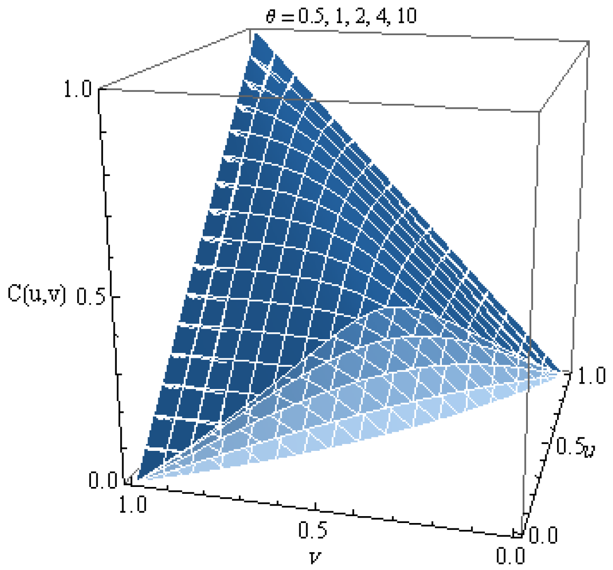
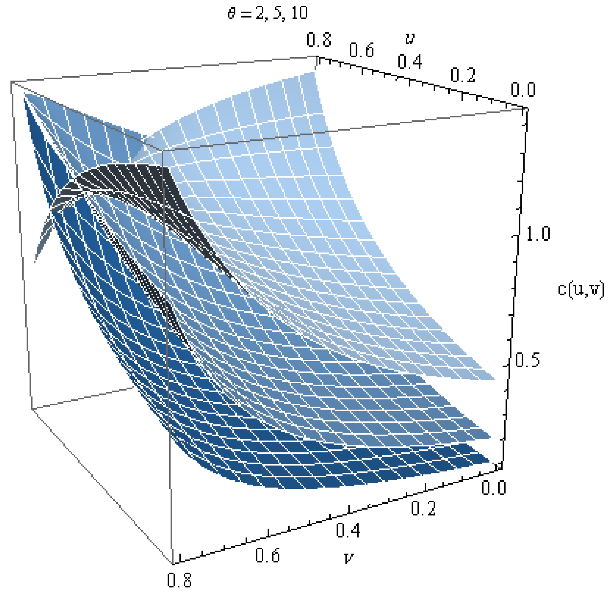
Example 1.

The cdf of the exponential distribution restricted to I is $F\left(x\right)=\frac{1-e^{-\theta x}}{1-e^{-\theta }},$ $0\le x\le 1$ and $\theta >0$, which has decreasing pdf as $f\left(x\right)=\frac{\theta e^{-\theta x}}{1-e^{-\theta }}$. Therefore, using Theorem 3, we could use $\overline{F}\left(x\right)=\frac{e^{-\theta x}-e^{-\theta }}{1-e^{-\theta }}$ as an additive Archimedean generator; which constructs the copula

$$C(u,v)=\left\{\begin{array}{cc}-\frac{1}{\theta }ln(e^{-\theta u}+e^{-\theta v}-e^{-\theta }),\hfill & if{e}^{-\theta u}+e^{-\theta v}-e^{-\theta }\le 1\hfill \\ 0,\hfill & Otherwise\hfill \end{array}\right.;0\le u,v\le 1.$$

(2)

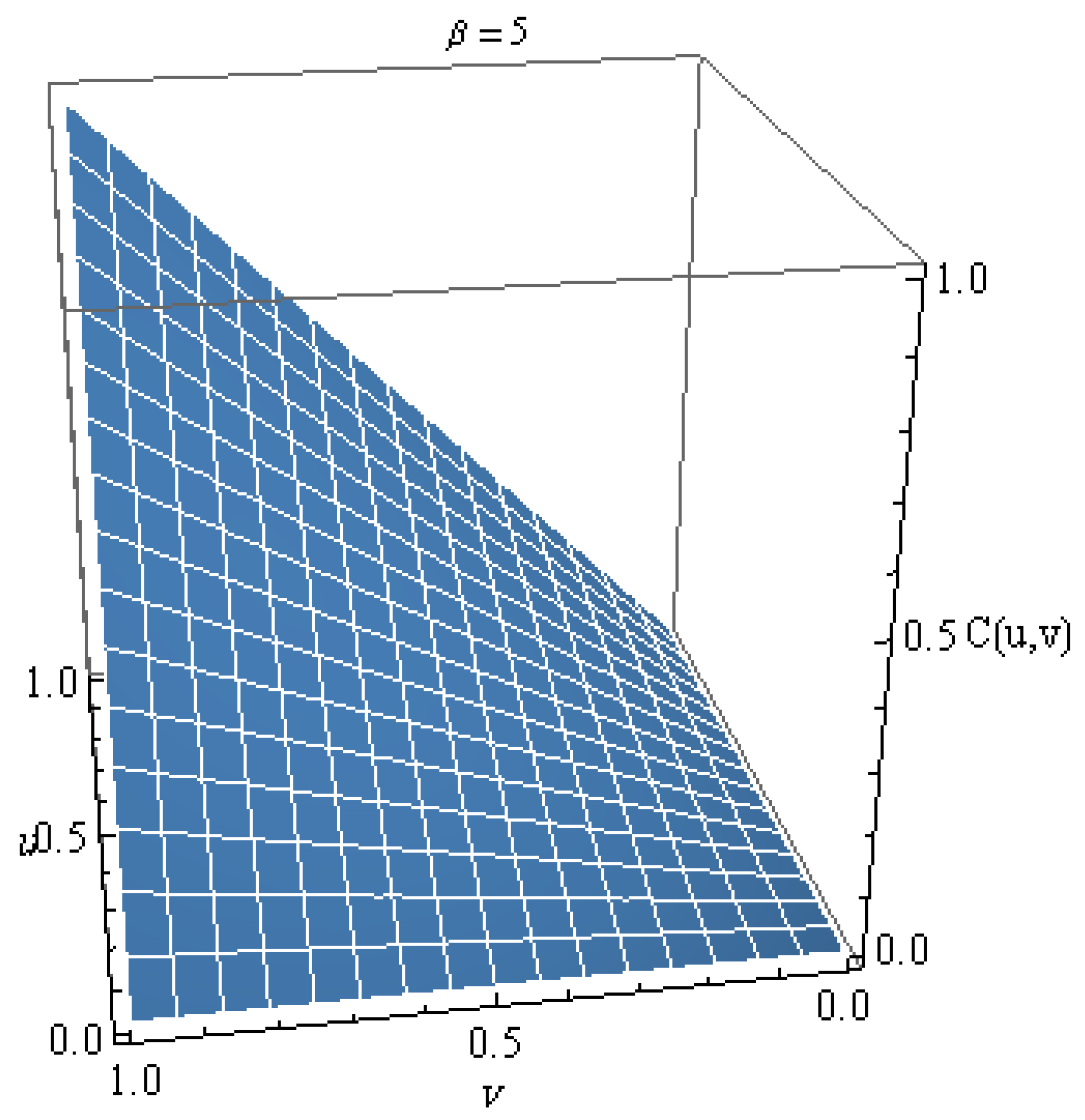
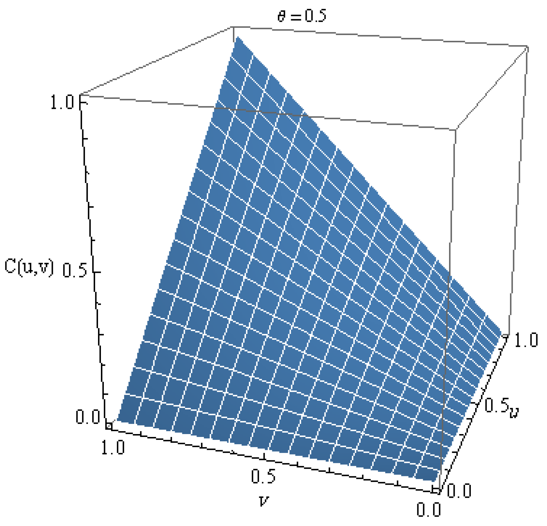
The plot of this copula for different values of $\theta$ is shown in Figure 1. From the graph, we can notice that this copula is increasing in $\theta$. Figure 2 shows the density for several values of $\theta$, where the density copula is given by

$$c(u,v)=\frac{\theta e^{-\theta (u+v)}}{{(e^{-\theta u}+e^{-\theta v}-e^{-\theta })}^2},if{e}^{-\theta u}+e^{-\theta v}-e^{-\theta }\le 1;0\le u,v\le 1.$$

Now, consider the function $H\left(x\right)=1-F(1-x)$. Then, $\overline{H}\left(x\right)=1-H\left(x\right)$ is additive Archimedean generator if $h\left(x\right)=f(1-x)$ is decreasing or equivalently $f\left(x\right)$ is increasing. Hence, we have the following corollary.

Corollary 1.

If F is a strictly increasing cdf on I with increasing pdf f, then

$$C(u,v)=\left\{\begin{array}{cc}1-F^{-1}(F(1-u)+F(1-v)),\hfill & ifF(1-u)+F(1-v)\le 1\hfill \\ 0,\hfill & Otherwise\hfill \end{array}\right.;0\le u,v\le 1$$

is a copula.

Now moving to multiplicative Archimedean generating functions, we observe that a strictly increasing cdf on I is a multiplicative Archimedean generator if F is log-concave. Therefore, we have the following theorem.

Theorem 4.

If F is a strictly increasing log-concave cdf on I, then

$$C(u,v)=F^{-1}\left(F\left(u\right)F\left(v\right)\right);0\le u,v\le 1$$

is a copula.

Proof. 

Note that the condition that F is log-concave together with the properties of distribution function make F a multiplicative Archimedean generator. Hence, the result follows. □

Also, if F is a cdf on I then $F^{-1}$ also a cdf. Therefore, we can get a multiplicative Archimedean generator using $F^{-1}$. This result is stated in the following theorem.

Theorem 5.

Let F be a continuous strictly increasing cdf on I with density $f\left(x\right)$. Suppose that $xf\left(x\right)$ is increasing on I then the function

$$C(u,v)=F\left(F^{-1}\left(u\right)F^{-1}\left(v\right)\right);0\le u,v\le 1$$

is a copula.

Proof. 

As F is cdf on I then $F^{-1}$ is also a cdf on I. Therefore, from Theorem 4, $F^{-1}\left(x\right)$ is multiplicative Archimedean generator if $F^{-1}$ is log-concave. But

$$\frac{d}{dx}ln\left(F^{-1}\left(x\right)\right)=\frac{1}{F^{-1}\left(x\right)f\left(F^{-1}\left(x\right)\right)}.$$

Thus, $F^{-1}\left(x\right)$ is log concave if and only if $\frac{1}{xf\left(x\right)}$ is decreasing or equivalently $xf\left(x\right)$ is increasing. □

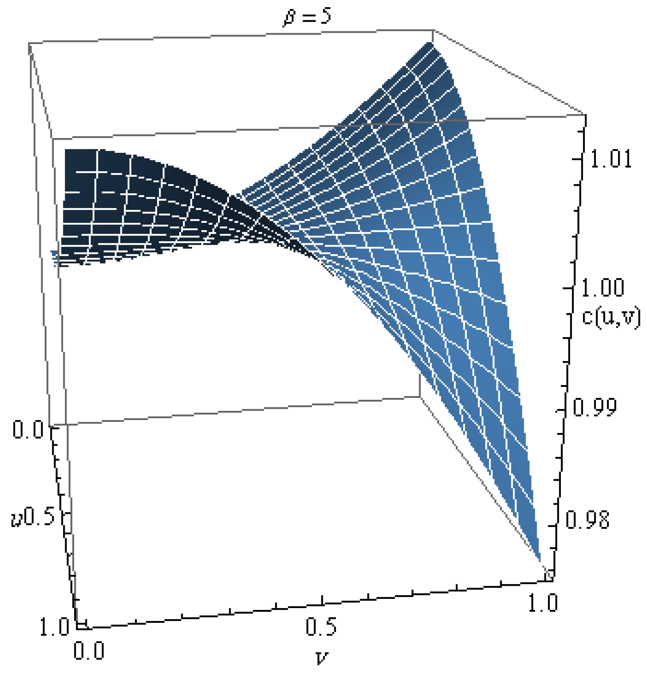
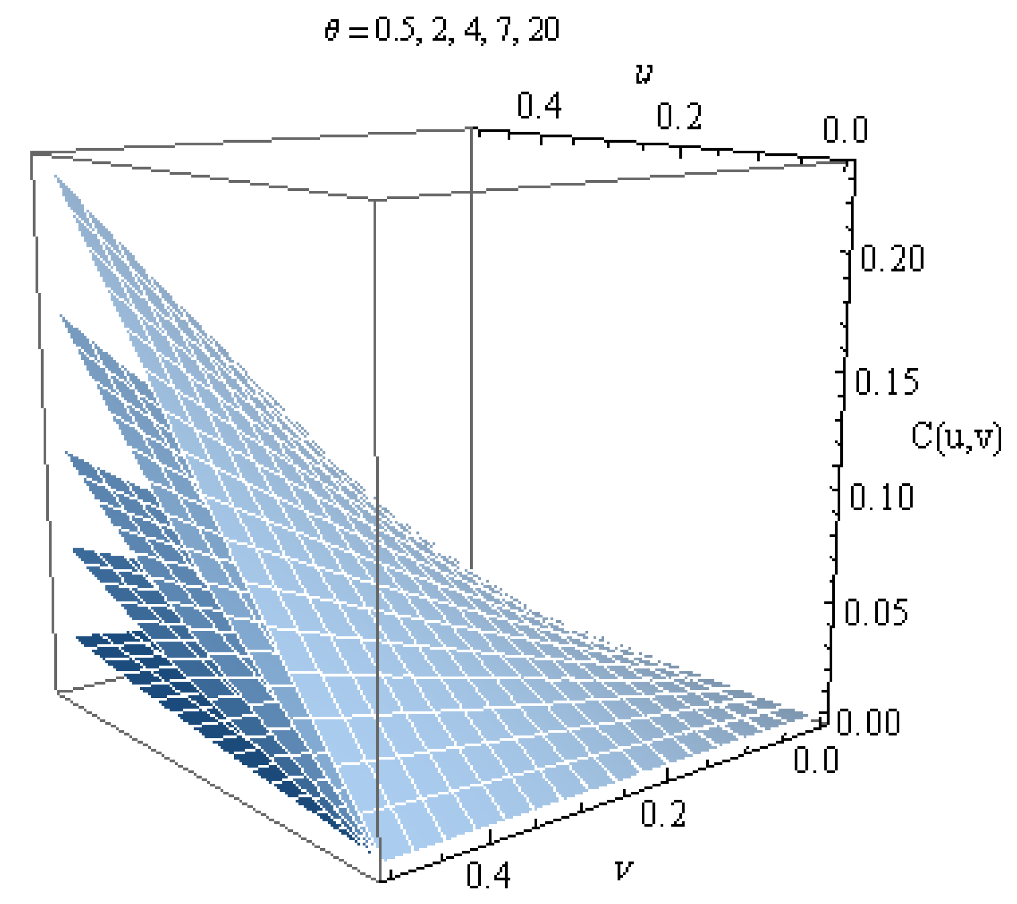
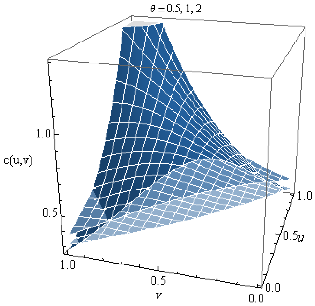
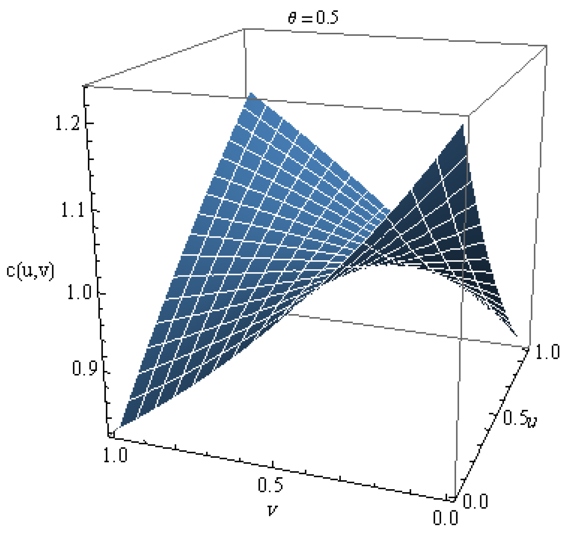
Example 2.

Consider the case of Gumbel distribution restricted to I, where $F\left(x\right)=\frac{e^{-e^{-\frac{x}{\beta }}}-e^{-1}}{c}; c=e^{-e^{-\frac{1}{\beta }}}-e^{-1}, \beta >1$. It is easy to check that $xf\left(x\right)$ is increasing. Thus, $F^{-1}\left(x\right)=-\beta ln\left[-ln(cx+e^{-1})\right]$ is multiplicative Archimedean generator, with the corresponding copula

$$C(u,v)=\frac{e^{-e^{-\beta ln[-ln(cu+e^{-1})]ln[-ln(cv+e^{-1})]}}-e^{-1}}{c};\beta >1,0\le u,v\le 1.$$

(3)

The copula and its density are depicted in Figure 3 and Figure 4, respectively.

Example 3.

Consider the density of Beta distribution $f\left(x\right)=\alpha {(1-x)}^{\alpha -1}$ with $\alpha <1$. This density satisfies $xf\left(x\right)$ is increasing. Then, the inverse of the cdf $F^{-1}\left(y\right)=1-{(1-y)}^{\frac{1}{\alpha }}$ is a multiplicative Archimedean generator. Hence, the corresponding multiplicative Archimedean copula is

$$C(u,v)=1-{\left[{(1-u)}^{\alpha }+{(1-v)}^{\alpha }-{(1-u)}^{\alpha }{(1-v)}^{\alpha })\right]}^{\frac{1}{\alpha }};0\le u,v\le 1.$$

This is known, in literature, as Joe copula.

Example 4.

Consider the distribution function discussed in Example 1, as $F\left(x\right)=\frac{1-e^{-\theta x}}{1-e^{-\theta }},\theta >0$. It can be easily verified that $F\left(x\right)$ is log concave, also for $\theta <1$, $xf\left(x\right)$ is increasing in I. We have $F^{-1}\left(t\right)=-\frac{1}{\theta }ln\left[-(1-e^{-\theta })t\right]$. Therefore, the two multiplicative Archimedean copulas corresponding to Theorem 4 and Theorem 5, respectively, are

$$C_1(u,v)=-\frac{1}{\theta }ln\left[1-\frac{(1-e^{-\theta u})(1-e^{-\theta v})}{1-e^{-\theta }}\right];\theta >0,0\le u,v\le 1;$$

and

$$C_2(u,v)=\frac{1-e^{-\frac{1}{\theta }ln\left[1-(1-e^{-\theta })u\right]ln\left[1-(1-e^{-\theta })v\right]}}{1-e^{-\theta }};0<\theta <1,0\le u,v\le 1.$$

(4)

The first copula is the well-known Frank copula with positive dependence parameter, while the second one is a new copula. The pdf of $C_2(u,v)$ is given by

$$c_2(u,v)=\frac{(1-e^{-\theta })e^{-\frac{1}{\theta }ln\left[1-(1-e^{-\theta })u\right]ln\left[1-(1-e^{-\theta })v\right]\left(1-\frac{1}{\theta }ln\left[1-(1-e^{-\theta })u\right]ln\left[1-(1-e^{-\theta })v\right]\right)}}{\theta \left[1-(1-e^{-\theta })u\right]\left[1-(1-e^{-\theta })v\right]};0\le u,v\le 1.$$

Figure 5 and Figure 6, give plots of the new copula and its density, respectively. It appears from the graph that this copula is decreasing in θ.

As applications of the cdf criteria to define copulas, we listed in

Table A1. Some copulas generated by survival functions $\overline{F}$.

Distribution	Generator	Parameter	Copula
Beta$(1,\beta )$	${(1-x)}^{\beta }$	$\beta <1$	$max\{0,1-{\left[{(1-u)}^{\beta }+{(1-v)}^{\beta }\right]}^{\frac{1}{\beta }}\}$
Beta$(\alpha ,1)$	$1-x^{\alpha }$	$\alpha <1$	$max\{0,{(u^{\alpha }+v^{\alpha }-1)}^{\frac{1}{\alpha }}\}$
Truncated BetaPrim$(1,\beta )$	$\frac{{(1+x)}^{-\beta }-2^{-\beta }}{1-2^{-\beta }}$	$\beta >0$	$max\{0,{\left[{(1+u)}^{-\beta }+{(1+v)}^{-\beta }-2^{-\beta }\right]}^{-\frac{1}{\beta }}-1\}$
Exponential-Logarithmic$(1,p)$	$\frac{ln\left(\frac{1-q{e}^{-x}}{1-q{e}^{-1}}\right)}{ln\left(\frac{p}{1-q{e}^{-1}}\right)}$	$0<p<1,$$q=1-p$	$max\{0,-ln\left[\frac{1}{q}+\frac{(q{e}^{-u}-1)(q{e}^{-v}-1)}{q(q{e}^{-1}-1)}\right]\}$

,

Table A2. Some copulas generated by $\overline{H}\left(x\right)=F(1-x)$.

Distribution	Generator	Parameter	Copula
Beta$(1,\beta )$	$1-x^{\beta }$	$\beta >1$	$max\{0,{(u^{\beta }+v^{\beta }-1)}^{\frac{1}{\beta }}\}$
Beta$(\alpha ,1)$	${(1-x)}^{\alpha }$	$\alpha >1$	$max\{0,1-{\left[{(1-u)}^{\alpha }+{(1-v)}^{\alpha }\right]}^{\frac{1}{\alpha }}\}$

and

Table A3. Some copulas generated by inverses of distribution functions $F^{-1}$.

Distribution	Generator	Parameter	Copula
Beta$(\alpha ,1)$	$x^{\frac{1}{\alpha }}$	$\alpha >0$	$uv$
Lomax$(1,\beta )$	$\frac{\beta x}{1+\beta -x}$	$\beta >1$	$\frac{uv}{1+\frac{1}{\beta }(1-u)(1-v)}$

of the Appendix A some well-known copulas with their corresponding generators.

4. Probability Generating Functions as Multiplicative Archimedean Generators

Probability generating functions (pgfs) are quite important tools due to their numerous uses. Mainly, the pgf could be used to drive the probability mass function for all possible values of the random variable and their moments. Moreover, a discrete random variable is totally determined by its pgf. For some cases, the use of pgf gives easy way to drive the distribution of the sum of two independent discrete random variables. Here, we demonstrate the use of pgfs as a class of multiplicative Archimedean generators. A sufficient condition for pgf to be a multiplicative Archimedean generator is given in terms of its probability mass function. Some well-known copulas and new ones are derived using pgfs. At first, we will present some preliminary definitions and related properties.

Definition 5.

Let X be a discrete random variable with distribution $P(X=k)=p_k,k\in Z_0^{+}$. Then the probability generating function (pgf) G of X is defined by

$$G\left(s\right)=E\left[s^X\right]=\sum _{k=0}^{\infty }{p}_k{s}^k,$$

where $s\in [0,1]$.

Note that, $G\left(0\right)=p_0$, $G\left(1\right)=1$ and $G^{\left(i\right)}\ge 0,i=0,1,\dots$; i.e., G is absolutely monotonic function on I. Hence, it is strictly increasing convex distribution function in I with jump $p_0$ at zero. However, in the case $p_0>0$, we may overcome this obstacle, if it is needed, by considering $G^{*}\left(s\right)=\frac{G\left(s\right)-p_0}{1-p_0}$ or $G^{**}\left(s\right)=sG\left(s\right)$. It is obvious that $G^{*}$ and $G^{**}$ are both continuous distribution functions on I. While $p_0=0$ implies that $G:I\to I$ is continuous, strictly increasing function, with $G\left(0\right)=0$ and $G\left(1\right)=1$. Then based on Theorem 4, we have the following theorem

Theorem 6.

If a pgf G is log-concave then the function

$$C(u,v)=G^{-1}\left(G\left(u\right)G\left(v\right)\right);0\le u,v\le 1$$

is a copula.

Note that, if $G\left(0\right)\ne 0$, then, $G^{[-1]}\left(G\left(t\right)\right)=t$, but $G\left(G^{[-1]}\left(t\right)\right)=max[t,G\left(0\right)]$.

Example 5.

Consider the pgf for zero-truncated Poisson distribution $G\left(s\right)=\frac{e^{\mu s}-1}{e^{\mu }-1}$. Then its inverse is $G^{-1}\left(t\right)=\frac{1}{\mu }ln[1+(e^{\mu }-1)t]$.

Thus, applying Theorem 6, the corresponding copula is

$$C(u,v)=\frac{1}{\mu }ln\left[\frac{(1+(e^{\mu u}-1)(e^{\mu v}-1)}{e^{\mu }-1}\right];0\le u,v\le 1.$$

This is known as Frank copula with negative dependence parameter.

Before proceeding to the next theorem which discusses the condition on a pgf to be log-concave, there is need to define the following terms.

Definition 6.

A non-negative sequence $\left\{p_n\right\}$ is log-concave if

$$p_n^2\ge p_{n+1}{p}_{n-1}foralln\ge 1.$$

The condition of log-concavity could be rephrased as: For $n\ge 1$ the ratio $\frac{p_{n+1}}{p_n}$ is decreasing whenever $p_n>0$. In general, the pgf is not log-concave. Keilson [10] discussed the relationship between the log-concavity of probability sequence $\left\{p_n\right\}$ and its generating function. Here, we try to give a sufficient condition on $\left\{p_n\right\}$ for the log-concavity of the corresponding pgf. We need the following definitions.

Definition 7.

A non-negative sequence $\left\{p_n\right\}$ is ultra-log-concave if

$$n{p}_n^2\ge (n+1)p_{n+1}{p}_{n-1}foralln\ge 1.$$

An equivalent condition is that, for $n\ge 1$ the ratio $\frac{(n+1)p_{n+1}}{p_n}$ is decreasing whenever $p_n>0$. Note that, an ultra-log-concavity implies log-concavity. For more discussion, see the review paper [11].

The following theorem gives a sufficient condition for a pgf to be log-concave in terms of the corresponding probabilities.

Theorem 7.

Let G be a pgf of $\left\{p_n\right\}$. If $\left\{p_n\right\}$ is ultra-log-concave, then G is log-concave.

Proof. 

For proof see Appendix A. □

Remark 1.

Notice that the ultra-log-concavity condition in Theorem 7 cannot be replaced by log-concavity. Here is a simple illustrative example, let X be a discrete random variable having geometric distribution with parameter p. Note $p_n^2=p_{n-1}{p}_{n+1}$, and hence $\left\{p_n\right\}$ is log-concave (log-convex) sequence. However, the ultra-log-concavity condition is not applicable. Whereas its pgf $G\left(s\right)=\frac{p}{1-(1-p)s}$ is not log-concave (it is log-convex).

The next theorem considers the inverse of pgf as a multiplicative Archimedean generator.

Theorem 8.

If $G\left(0\right)=0$, then $G^{-1}$ is a strict multiplicative Archimedean generator. i.e.

$$C(u,v)=G\left(G^{-1}\left(u\right)G^{-1}\left(v\right)\right);0\le u,v\le 1$$

is a copula.

Proof. 

It is clear that the function $G^{-1}:I\to I$ is

• Continuous on I.
• Strictly increasing on I.
• $G^{-1}\left(1\right)=1$ and $G^{-1}\left(0\right)=0$.
• Log-concave. Because we have $\frac{d}{du}ln\left[G^{-1}\left(u\right)\right]=\frac{1}{G^{{}^{\prime }}\left[G^{-1}\left(u\right)\right]G^{-1}\left(u\right)}$ decreasing. Since both $G^{-1}\left(u\right)$ and $G^{{}^{\prime }}\left[G^{-1}\left(u\right)\right]$ are increasing.

Hence, Theorem 5, gives the result. □

Example 6.

Consider the pgf in Example 5. For easy notation, we set $\theta =e^{\mu }-1$, i.e. $\mu =ln(1+\theta )$. Therefore, $G\left(s\right)=\frac{e^{sln(1+\theta )}-1}{\theta }$, and hence, $G^{-1}\left(t\right)=\frac{ln(1+\theta t)}{ln(1+\theta )}$. Thus, applying Theorem 8, one gets the corresponding copula as

$$C(u,v)=\frac{1}{\theta }[e^{\frac{ln(1+\theta u)ln(1+\theta v)}{ln(1+\theta )}}-1];0<\theta <\infty ,0\le u,v\le 1.$$

(5)

Figure 7 and Figure 8, give plots of the copula and its density, respectively.

Now consider the function $W\left(s\right)=G(1-s)$. Then, W is decreasing and convex. Also, $W\left(0\right)=1$ and $W\left(1\right)=0$. Thus, it is a non-strict additive Archimedean generator. Hence, we can get the following result as an immediate consequence of Corollary 1.

Corollary 2.

If G is a pgf with $G\left(0\right)=0$, then $G(1-s)$ is an additive Archimedean generator with the corresponding copula

$$C(u,v)=\left\{\begin{array}{cc}1-G^{-1}(G(1-u)+G(1-v)),\hfill & ifG(1-u)+G(1-v)\le 1\hfill \\ 0,\hfill & Otherwise\hfill \end{array}\right.;0\le u,v\le 1.$$

Example 7.

Consider the pgf of truncated Poisson distribution $G\left(s\right)=\frac{e^{\mu s}-1}{e^{\mu }-1}$. Then, $W\left(s\right)=\frac{e^{-\mu s}-e^{-\mu }}{1-e^{-\mu }}$, which is the same as survival function of truncated exponential discussed in Example 1.

In

Table A4. Some famous copulas generated by probability generating functions and their inverses.

Distribution	Generator	Parameter	Copula
Binomial$(n,p)$	$G\left(s\right)={(1-p+ps)}^n$	$0<p<1$	$max\left\{\right(1-p\left)\right(u+v-1)+puv,0\}$
Geometric$\left(p\right)$	$G\left(s\right)=\frac{ps}{1-(1-p)s}$	$0<p<1$	$\frac{uv}{1+\frac{1-p}{p}(1-u)(1-v)}$
Poisson$\left(\mu \right)$	$G\left(s\right)=e^{\mu (s-1)}$	$\mu >0$	$max\{u+v-1,0\}$
Truncated Poisson$\left(\mu \right)$	$G\left(s\right)=\frac{e^{\mu *s}-1}{e^{\mu }-1}$	$\mu >0$	$\frac{1}{\mu }ln[1+\frac{(e^{\mu u}-1)(e^{\mu v}-1)}{e^{\mu }-1}]$
Pascal$\left(p\right)$	$G^{-1}\left(s\right)={\left[\frac{(1-p)s}{1-ps}\right]}^r$	$0<p<1$$r:$ Integer	$\frac{uv}{{\left[1-p\left(1-u^{\frac{1}{r}}\right)\left(1-v^{\frac{1}{r}}\right)\right]}^r}$

of the Appendix, we listed some well-known copulas with their corresponding generating pgfs.

5. Conclusions

In this paper, we viewed a cumulative distribution function and probability generating function as Archimedean generators. Sufficient conditions in terms of probability function were discussed. Some new copulas were given.