Automated Fitting Process Using Robust Reliable Weighted Average on Near Infrared Spectral Data Analysis

Abstract

With the complexity of Near Infrared (NIR) spectral data, the selection of the optimal number of Partial Least Squares (PLS) components in the fitted Partial Least Squares Regression (PLSR) model is very important. Selecting a small number of PLS components leads to under fitting, whereas selecting a large number of PLS components results in over fitting. Several methods exist in the selection procedure, and each yields a different result. However, so far no one has been able to determine the more superior method. In addition, the current methods are susceptible to the presence of outliers and High Leverage Points (HLP) in a dataset. In this study, a new automated fitting process method on PLSR model is introduced. The method is called the Robust Reliable Weighted Average—PLS (RRWA-PLS), and it is less sensitive to the optimum number of PLS components. The RRWA-PLS uses the weighted average strategy from multiple PLSR models generated by the different complexities of the PLS components. The method assigns robust procedures in the weighing schemes as an improvement to the existing Weighted Average—PLS (WA-PLS) method. The weighing schemes in the proposed method are resistant to outliers and HLP and thus, preserve the contribution of the most relevant variables in the fitted model. The evaluation was done by utilizing artificial data with the Monte Carlo simulation and NIR spectral data of oil palm (Elaeis guineensis Jacq.) fruit mesocarp. Based on the results, the method claims to have shown its superiority in the improvement of the weight and variable selection procedures in the WA-PLS. It is also resistant to the influence of outliers and HLP in the dataset. The RRWA-PLS method provides a promising robust solution for the automated fitting process in the PLSR model as unlike the classical PLS, it does not require the selection of an optimal number of PLS components.

1. Introduction

The Near Infrared Spectroscopy (NIRS) has recently been attracting a lot of attention as a secondary analytical tool for quality control of agricultural products. In some applications (see [1,2,3,4,5]), it has been proven that the NIRS offers a non-destructive, reliable, accurate, and rapid tool, particularly for quantitative and qualitative assessments. Theoretically, NIRS is a type of vibrational spectroscopic that produces rich information in a spectral dataset as a result of the interaction between optical light and the physical matter of the sample. This spectral is commonly presented in terms of spectral absorbance using wide wavelengths that range from 350 nm to 2500 nm, primarily attributed to the overtone or combination bands of C-H (fats, oil, hydrocarbons), O-H (water), and N-H (protein) [6]. The NIR spectral data are classified as high dimension due to the large sample size and wide wavelength collected as a dataset. In spectral processing, chemometric methods have been utilized as the standard processing method (see [7,8,9]). The methods combine the mathematical and multivariate statistical methods in order to pre-process, examine, and understand as much relevant information as possible from the spectral data. Comparing some of the existing chemometric methods, the Partial Least Squares Regression (PLSR) seems to be the most preferred one [10,11,12].

PLSR decomposes both the spectral and reference information (from wet chemistry analysis), simultaneously. It has the ability to screen unwanted samples in a dataset as a result of experimental error and instrumentation problem [13], distribution-free assumption [14,15], and handling the multicollinearity in dataset [16]. However, despite having these benefits, several studies have reported its weakness due to its robustness. The fitted model performs poorly when outliers and leverage points are present in a dataset [17,18], as it fails to fit the nonlinear behavior in the input space [19,20]. In addition, the contamination of irrelevant variables involves during the fitting process [21,22,23] is a popular topic in most discussions. However, so far, less attention has been paid to the basic principles of PLSR in selecting the optimal number of Partial Least Squares (PLS) components which is crucial [24]. Applying fewer number of components produced under fitting, while applying a large number of components results in over fitting. Some methods available in the selection procedure are the cross-validation with one-sigma heuristic [25], permutation approach [26], bootstrap [27], smoothed PLS–PoLiSh [28], weight randomization test [29], and Monte Carlo resampling [30]. These different methods suggest different optimal numbers of the PLS components and to date, there has been no claim made as to which method is superior to the other. These methods suffer from the presence outliers and High Leverage Points (HLP) in the dataset. Consequently, recalculation of the number of PLS components used in the model is required each time the dataset is updated. This would result in different accuracy achievements and sometimes, misleading interpretations. It has been observed that there are only a few studies that have highlighted the robust process. As such, a robust PLSR with less sensitivity to the selection of optimal number of PLS components is needed. This study provides another perspective of applying a robust procedure in the PLSR model with regard to the selection number of the factors used in the fitted model.

The automated fitting process on PLSR model using weighted average strategy has been introduced in several papers (see [31,32,33]). The method is known as the Locally Weighted Average PLS [31,32] or simply called the Local-WA-PLS. The Local-WA-PLS is an extension of the Locally Weighted Regression [33] which is used to fit a local linear regression based on the classification of similarity between the calibration and testing (or unknown) sample. This similarity is classified using the famous Euclidean distance and Mahalanobis distance method. Although the Local-WA-PLS has been widely used, it has been reported that the method works adequately only with a large spectral dataset (see [34,35]). As an improvement, the modified method by Zhang et al. [35], the Weighted Average PLS (WA-PLS), is suggested as it uses a different weighting scheme that is computationally simpler and comparable to the Local-WA-PLS. However, both methods are not able to handle the problems of outliers and HLP that may exist in the dataset from affecting their performances. In addition, the Local-WA-PLS and WA-PLS do not take into consideration the influence of some irrelevant variables in the model that might decrease their estimation accuracy. This has motivated the current study to propose another improvement to robustify the existing WA-PLS procedure. Our strategies were to employ the weighting schemes that are resistant to outliers and HLP and preserve the contribution of the most relevant variables in the fitted model. The utilization of the robust PLSR [36] is incorporated in the establishment of the proposed procedures.

The main objectives of this study are: (1) to establish an improved procedure for the automated fitting process in the PLSR model known as the Robust Reliable Weighted Average PLS (RRWA-PLS). This proposed method is expected to be less sensitive to the selection of the optimal number of PLS components; (2) to evaluate the performance of the proposed RRWA-PLS method with the classical PLSR using optimal number of PLS components, WA-PLS, and a slight modification method in WA-PLS using a robust weight procedure called MWA-PLS; (3) to apply the proposed method on the artificial data and NIR spectra of oil palm (Elaeis guineensis Jacq.) fruit mesocarp (fresh and dried ground). This study provides a significant contribution to the development of process control, particularly for research methodology in the vibrational spectroscopy area.

2. Materials and Methods

2.1. Partial Least Squares Regression

The PLSR model [14] is an iterative procedure of the multivariate statistical method. The method is used to derive $m$ original predictor variables $X$ that may have a multicollinearity problem into smaller uncorrelated $l$ new variables called components. The PLSR constructs a regression model using the new components against its response variable $\mathbf{y}$ through covariance structure of these two spaces. In chemometric analysis, the PLSR has been widely used for dimensional reduction of high dimensionality problem in the NIR spectral dataset (see [37,38]). In this study, we limited the study only in the case of $n>>m$, where $n$ refers to the number of observations, and $m$ represents the number of predictor variables.

Let us define a multiple regression model which consists of two different sets of multiple predictor $X$ and a single response $\mathbf{y}$,

$$y=X b + e$$

(1)

where $\mathbf{y}$, $e$ are $n\times 1$ vector; $X$ is $n\times m$ matrix; and $b$ is $m\times 1$ vector. Since the dataset contains high dimension of $m$ predictors, there will be an infinite number of solution for estimator $b$. Considering $X^{T}X$ is singular, it does not meet the usual trivial theorem on rank in the classical regression. To overcome this, new latent variables need to be produced by summarizing the covariance between predictor $X$ and response variable associating to the center values of these two sets [39].

Initializing a starting score vector of $u$ from the single $\mathbf{y}$; there exists an outer relation for predictor $X$ in Equation (1) as

$$X=V{P}^T+E$$

(2)

where $V$ is a $n \times l$ (for $l\le m$) matrix of the $n\times 1$ vector $v_g$${\left\{v_g=\left(X w_j\right)/\left(w_j{}^T{w}_j\right)\right\}}_{ g=1}^{ l}$; and $v_g$ is the $n\times 1$ column vector of scores $x_j$ in $X$. The $P$ is a $m\times l$ matrix consisting column vector of loading ${\left\{p_g=\left(X^T v_g\right)/\left(v_g{}^T{v}_g\right)\right\}}_{g=1}^l$. The $w_j$${\left\{w_j=\left(X^{T}u\right)/\left(u^{T}u\right)\right\}}_{ j=1}^{ m}$ is a $m\times 1$ vector of weight for $X$ and $E$ is a $n\times m$ matrix of residual in outer relation for $X$. In addition, there is a linear inner relation between the $X$ and $\mathbf{y}$ block scores, calculated as ${\left\{u= b_g v_g, b_g=u_{}^T v_g/\left(v_g^T v_g^{}\right)\right\}}_{ g=1}^l$ or written as

$$u = V b_{inner}+g$$

(3)

with $b_{inner}$ is a $l\times 1$ vector of regression coefficient as the solution using Ordinary Least Square (OLS) on the decomposition of vector $u$, and $g$ is $n\times 1$ vector of residual in the inner relation. Following the Nonlinear Iterative Partial Least Squares (NIPALS) algorithm (see [14]), the mixed relation in the PLSR model can be defined as

$$y = X b_{PLSR}+\stackrel{⌣}{f}$$

(4)

where $b_{PLSR}=W {(P^{T}W)}^{-1}a$ is $m\times 1$ vector coefficient; $a$ represents $l\times 1$ vector coefficient which is $a=V^{T}y$; and $\stackrel{⌣}{f}$ denotes $n\times 1$ vector of residual in mixed relation that has to be minimized. The estimator for parameter $b_{PLSR}$ is given as

$${\hat{b}}_{PLSR}=X^{T}u {(V^{T}X X^{T}u)}^{-1}{V}^{T}y, {\hat{b}}_{PLSR}\in {\Re }^{m\times 1}$$

(5)

with ${\hat{b}}_{PLSR}$ denotes $m$ dimensional vector of regression coefficient in PLSR.

2.2. Partial Robust M-Regression

An alternative robust version of PLSR introduced by Serneel et al. [36] is the partial robust M-regression or simply known as PRM-Regression. The method assigns a generalized weight function $w_i$ using a modified robust M-estimate [40]. This weight is obtained from the iterative reweighting scheme (see [41]) to identify the outliers and HLP, both in each observation and score vector $v_i$. Let us consider the $m$ regression in Equation (1), for $1\le i\le n$, the least square estimator of $b$ is defined as

$${\hat{b}}_{LS}=\underset{b}{\arg \min }\left({\displaystyle \sum _{i=1}^n{\left(y_i-x_i b\right)}^2}\right)$$

(6)

The least square is optimal if $E \left(e\right)=0$ and $Var \left(e\right)=1$ or where $e~N\left( 0 , 1 \right)$; otherwise, it fails to satisfy the normal assumption. When it does not satisfy this assumption, the least square losses its optimality; hence, a robust estimator such as M-estimates results in a better solution.

In Serneels et al. [36], the robust M-estimates reestablish the squares term into $u$ giving

$${\hat{b}}_M=\underset{b}{\arg \min }\left({\displaystyle \sum _{i=1}^n\theta \left(y_i-x_{i}b\right)}\right)$$

(7)

where $\theta \left(u\right)=u^2$, $\theta \left(y_i-x_{i}b\right)={\left(y_i-x_i b\right)}^2$ as $\theta \left(u\right)$ is defined to be loss function which is symmetric and nondecreasing. Recall the $e$ as residual $n\times 1$ column vector ${\left\{e_i=y_i-x_i b\right\}}_{i=1}^n$ related to Equation (7), then ${\hat{b}}_M=\underset{b}{\arg \min }\left({\displaystyle \sum _{i=1}^n\theta \left(e_i\right)}\right)$. Using partial derivative and following the iterative reweighting scheme, there exists a weight in each observation as $w_i^r=\theta (e_i)/e_i{}^2$, taking $\theta (e_i)=w_i^r e_i{}^2$, the Equation (7) can be rewritten as

$${\hat{b}}_M=\underset{b}{\arg \min }\left({\displaystyle \sum _{i=1}^n{w}_i^r e_i{}^2}\right)$$

(8)

It is considered that the weight in Equation (8) is only sensitive to the vertical outlier as improvement of another weight $w_i^x$ is added to identify the leverage points. The criteria $w_i^x\approx 0$ would be identified as the leverage points. The modified final estimator in Equation (8) is given as

$${\hat{b}}_{RM}=\underset{b}{\arg \min }\left({\displaystyle \sum _{i=1}^n{w}_i^r w_i^x e_i{}^2}\right)$$

(9)

where $w_i^{}=w_i^r w_i^x$ is the generalized weight. Replacing the residual in Equation (9) with $n\times 1$ vector of residual in Equation (4), then giving the solution of the partial robust M-regression as

$${\hat{b}}_{PRM}=\underset{b}{\arg \min } \left({\displaystyle \sum _{i=1}^n{w}_i^r w_i^x {\stackrel{⌣}{f}}_i{}^2}\right)$$

(10)

with the weights $w_i^r$ and $w_i^x$ are given as

$$w_i^r=f \left(\frac{{\stackrel{⌣}{f}}_i}{\hat{\sigma }},c\right)$$

(11)

where $\hat{\sigma }$ uses the robust $\mathrm{MAD} \left({\stackrel{⌣}{f}}_1,\dots ,{\stackrel{⌣}{f}}_n\right)=\underset{i}{\mathrm{median}}|{\stackrel{⌣}{f}}_i-\underset{j}{\mathrm{median} {\stackrel{⌣}{f}}_j|}$, $f \left(z,c\right)$ is the weight function of iterative reweighting.

$$w_i^x=f\left(\frac{\left|\right|v_i-{\mathrm{med}}_{L1}\left(V\right)\left|\right|}{\mathrm{median}\left|\right|v_i-{\mathrm{med}}_{L1}\left(V\right)\left|\right|},c\right)$$

(12)

$\left|\right|\cdot \left|\right|$ is Euclidean norm; ${\mathrm{med}}_{L1}\left(V\right)$ is a robust estimator of the center of the $l$ dimensional score vectors; and $v_i={(v_{i,1},\dots ,v_{i,l})}^T$ is the vector of component score matrix $V$ that needs to be estimated. The fair weight function in $f \left(z,c\right)$ is preferred instead of other weights.

2.3. Weighted Average PLS

The WA-PLS method was introduced by Zhang [35] to encounter the sensitivity of PLSR toward the specific number of PLS components used. The method applies the averaging strategy to accommodate the whole possible complexity of the model. This complexity means that some models were initiated based on the increase from the $r$th to the $s$th number of PLS components used in the fitting model. Instead of applying the same weight in each PLSR model, the WA-PLS proposes different weights $w_r$ using variance weighting to each coefficient $b_{PLSR}=\left[b_1,b_2,\dots ,b_m\right]$ in the $d$ PLSR model $\left\{d=s-r\right\}$ with the complexity of $r$.

$$w_r=\frac{1}{RMSEC{V}_r}$$

(13)

where the Root Mean Square Error Cross Validation (RMSECV) in each different number of $r$th PLS components is calculated as

$$RMSEC{V}_r=\sqrt{\frac{1}{n}{\displaystyle \sum _{i= 1}^n {\left(y_i-{\hat{y}}_{\backslash i,r}\right)}^2}}$$

(14)

where ${\hat{y}}_{\backslash i,r}$ is the predicted value of the actual value of $y_i$ using the fitted model which is built without sample $i$ and is under the complexity of $r$. The WA-PLS formula using weight and average from $r$th to the $s$th number of PLS components can then be written as

$$\begin{array}{ll}{\overline{\hat{y}}}_{WA-PLS \left(r, s\right)}& =\left[\frac{w_r{b}_{0,r}^{}+\dots +w_s{b}_{0,s}^{}}{w_r+\dots +w_s}\right] +\left[\frac{w_r{b}_{1,r}^{}+\dots +w_s{b}_{1,s}^{}}{w_r+\dots +w_s}\right] x_1+\\ & \hspace{1em}\hspace{1em}\left[\frac{w_r{b}_{2,r}^{}+\dots +w_s{b}_{2,s}^{}}{w_r+\dots +w_s}\right] x_2+\dots +\left[\frac{w_r{b}_{m,r}^{}+\dots +w_s{b}_{m,s}^{}}{w_r+\dots +w_s}\right] x_m\end{array}$$

(15)

3. Robust Reliable Weighted Average

Following Zhang’s et al. [35] weighted average calculation on each coefficient of $d$ different numbers of PLS components, a robust version of the modified weighted average is developed. The method is called the Robust Reliable Weighted Average (RRWA) which accommodates two weights $(w_r,c_j)$ in the calculation of the PLSR model. It is expected that by assigning the weighted average method in the PLSR model, the model becomes less sensitive to the number of PLS components used.

In the first weight $w_r$, the calculation uses the Standard Error Prediction (SEP) which is done iteratively based on the re-sampling procedure of $k$-fold cross validation by splitting a dataset into $k$-subsets [42]. This procedure is the most used approach to retrieve a good estimate of error rate in the model selection. Nonetheless, it is anticipated that 20% of the highest absolute values of residuals may still be included in the calculation of $w_r$. In order to remove those residuals, the trimmed version (20%) SEP from the cross validation ($trimmed SEPC{V}_r$) is applied. The assigned weight $w_r$ to each coefficient of $d$ different numbers of PLS components is calculated as

$$w_r=\frac{1}{trimmed SEPC{V}_r}$$

(16)

where the $trimmed SEPC{V}_r$ values are calculated using the collection of the $SE{P}_r$ from $k$-subsets starting from $r$th to the $s$th number of PLS components. The calculation for $SE{P}_r$ is given as

$$SE{P}_r=\sqrt{\frac{1}{n-1}{\displaystyle \sum _{i=1}^n{\left(e_{ir}- {\overline{e}}_r\right)}^2}}$$

(17)

where $e_{ir}$ is the residual from predicted value of ${\hat{y}}_{\backslash i,r}$ and actual value of $y_i$ with the complexity of $r$, and ${\overline{e}}_r$ is the arithmetic mean of the residuals. It corresponds to the $MSE{P}_r^{}=SE{P}_r^2+ {\overline{e}}_r^2$ where the bias is identically equal to 0, then the $MSE{P}_r^{}$ is equals to $SE{P}_r^2$. While the bias is identically (almost) zero, the squared root of $MSE{P}_r^{}$ which is

$$RMSE{P}_r=\sqrt{\frac{1}{n}{\displaystyle \sum _{i=1}^n{e}_{ir}{}^2}}$$

(18)

is (almost) equal to the $SE{P}_r$. This alternative weight could be called as a modified weight in WA-PLS, and is simply denoted as the MWA-PLS method which is also included as an alternative proposed method in this study.

In the classical WA-PLS, the number of possible irrelevant variables is still involved in the model. Eliminating these irrelevant variables would result in under or over fitting. Here, a downgrading procedure by assigning the second weight $c_j$ to each variable in terms of reliability values [21] is proposed. The procedure is based on the PLSR coefficient that is applicable to increase the contribution of most relevant variables in the model, and downgrade the irrelevant variables. The reliability of each variable $c_j$ is obtained by

$$c_j=\frac{\mathrm{median} \left(b_{j,r},\dots ,b_{j,s}\right)}{\mathrm{MAD} \left(b_{j,r},\dots ,b_{j,s}\right)}$$

(19)

where the calculation is based on the robust measure of central tendency and the robust measure of variability on each $j$th WA-PLS coefficient from $r$th to the $s$th numbers of PLS components. The robust weight $w_r$ in Equation (16) is preferred instead of the weight in Equation (13). In relation to the PLSR model, this reliability value $c_j$ is converted into a diagonal matrix with size $m\times m$. This diagonal matrix $\Omega$${\left\{\Omega =\mathrm{diag}\left(c_1,c_2,\dots ,c_m\right)\right\}}_s$ where $\Omega \in \Re$ is then used to transform the original input $X$ variables into the scaled input variables $\tilde{X}$$\left\{\tilde{X}=X \Omega \right\}$ for the RRWA-PLS model.

To prevent the influence of outliers and HLP that may exist in the NIR spectral dataset, the calculation of $trimmed SEPC{V}_r$ and reliability values are based on the PRM regression coefficient through a cross-validation procedure. The proposed modification of the WA-PLS known as the RRWA-PLS can be rewritten as

$$\begin{array}{ll}{\overline{\hat{y}}}_{RRWA-PLS \left(r, s\right)}=& \left[\frac{w_r{b}_{0,r}^{\prime }+\dots +w_s{b}_{0,s}^{\prime }}{w_r+\dots +w_s}\right] +\left[\frac{w_r{b}_{1,r}^{\prime }+\dots +w_s{b}_{1,s}^{\prime }}{w_r+\dots +w_s}\right] {\tilde{x}}_1+\\ & \left[\frac{w_r{b}_{2,r}^{\prime }+\dots +w_s{b}_{2,s}^{\prime }}{w_r+\dots +w_s}\right] {\tilde{x}}_2+\dots +\left[\frac{w_r{b}_{m,r}^{\prime }+\dots +w_s{b}_{m,s}^{\prime }}{w_r+\dots +w_s}\right] {\tilde{x}}_m\end{array}$$

(20)

where $b_j^{\prime }$ is the RRWA-PLS coefficient using the scaled input variables $\tilde{X}$.

4. Monte Carlo Simulation Study

To examine the performance of the proposed RRWA-PLS and to compare its performance with the classical WA-PLS and MWA-PLS, a study using the Monte Carlo simulation was carried out. Following a simulation study by Kim [43], an artificial dataset which contained added noise that follows the Normal distribution was randomly generated using a Uniform distribution and included. This dataset was then applied in the linear combination equation with different scenarios. Three sample sizes ($n =$ 60, 200, 400), three levels of numbers of predictor variables ($m =$ 41, 101, 201), three levels of relevant variables ($IV =$ 0.1, 0.3, 0.5), and three different levels of outliers and high leverage points ($\alpha =$ 0.00, 0.05, 0.20) were considered. The $100(IV)\%$ of the predictor variables were randomly selected as relevant variables, and the remaining were considered as less relevant. The formulation of this simulation can be defined as follows:

$$\begin{array}{ll}m=mo+me& \\ c_{j^o }~ U \left(1, 10\right)& \left(j^o=1, 2, \dots , mo\right)\\ c{e}_{j^e} ~ U \left(5, 20\right)& \left(j^e=1, 2, \dots , me\right)\\ e_j ~ N\left(0, 1\right)& \left(j=0, 1, 2,\dots , m\right)\\ b ~U(0,7)\\ iv = \left\{ i{v}_1,i{v}_2,\dots , i{v}_{100(IV)\%\ast m} \right\}\\ X =\left\{ c_{j^o},c{e}_{j^e} \right\}+e_j& \left(j=1, 2,\dots , m;j^o=1, 2, \dots , mo;j^e=1, 2, \dots , me\right)\\ y = X b +e_0& \left(i=1, 2,\dots , n;j=i{v}_1,i{v}_2,\dots , i{v}_{100(IV)\%\ast m}\right)\end{array}$$

(21)

where $m$ is the total number of predictors used; $mo$ is the number of observable variables; and the $me$$\left\{ me=\left(m-100 \left(IV\right)\%\ast m\right)/2\right\}$ is the number of artificial noise variable. These artificial variables are applied to evaluate the stability of the methods. The $c_{j^o}$ follows the Uniform distribution (1,10) with size $n$. The artificial noise variables $c{e}_{j^e}$ are added to the predictor and follow the Uniform distribution (5,20) with size $n$. This $c{e}_{j^e}$ is classified as an irrelevant variable. The $e_j$ follows the standard normal distribution with size $n$, and $b$ represents a vector coefficient for selected relevant variables which follows the Uniform distribution (0,7) with size $m$. The $c_{j^o}$, $c{e}_{j^e}$ and $e_j$ are independent of each other. The $iv$ is the set of selected relevant variables in $mo$, and $e_0$ is the added error in the linear combination of $\mathbf{y}$. $X$ and $\mathbf{y}$ are illustrated as observable variables. The high leverage points in the $X$ dimensions are created by generating $c_{j^o}$ following the Uniform distribution (1,10) with size $n$. Corresponding to the vertical outlier, if the observation is considered as an outlier, $b$ follows the Uniform distribution (0,2) with size $100 \left(IV\right)\%\ast m$; otherwise, it is considered as high leverage points and $b$ follows the Uniform distribution (1,7) with size $100 \left(IV\right)\%\ast m$. The different ranges applied in the uniform distribution are used to fit the different scenarios according to the added artificial noise, vertical outliers, and high leverage points in the dataset. By default, the predictor and response variable should be centered and scaled before the analysis. In the PLSR model, the selection on optimal number of PLSR components used in the model fitting is very important to prevent the model from becoming over- or under-prediction.

To assess the performance of the methods, several statistical measures such as desirability indices are used: Root Mean Square Error (RMSE), Coefficient of Determination (R²), and Standard Error (SE). The RMSE measures the absolute error of the predicted model; R² is the proportion of variation in the data summarized by the model and indicates the reliability of the goodness of fit for model; and SE measures the uncertainty in the prediction. Here, the RPD parameter has no more used because it is not different than R² to classify the model is poor or not [44]. Using the classical PLSR, the RMSECV which is the RMSE obtained through cross-validation, is calculated, along with the increasing number of PLS components. The RMSEP value is the RMSE obtained using the fitted model. In the simulation study, the maximum number of PLS components used was limited up to 20. Some different scenarios were applied to see the stability of classical PLSR model based on sample size, number of predictors, number of important variables, and the contamination of outlier and high leverage points in the dataset. In Figure 1, with no contamination in the data it can be seen that using small sample size ($n$ = 60), small number of predictors ($m$ = 41), and 10% relevant variable ($IV$ = 10%) the discrepancy between RMSECV and RMSEP is about two to five times. While using higher number of predictors ($m$ = 101) the discrepancy then become larger. Another scenario using bigger sample size ($n$ = 200), small number of predictors ($m$ = 41), and 30% relevant variable ($IV$ = 30%) the discrepancy between RMSECV and RMSEP relatively smaller. While using higher number of predictors ($m$ = 101) the discrepancy increases about two times. This shows that the classical PLS become instable and loss it accuracy when the number of sample size is small and number of predictor higher than sample size. In addition, with less number of relevant variable in the predictor variable also impacts to decrease the model accuracy. Using bigger sample size (for example $n$ = 200) as the number of PLS components increases the discrepancy between RMSECV and RMSEP become smaller hence improve the model accuracy and reliability. The rule is the gap between RMSEC and RMSEP values should very small and close to 0. This condition guarantees the reliability of the calibrated model and prevent the model becomes over-under fitting.

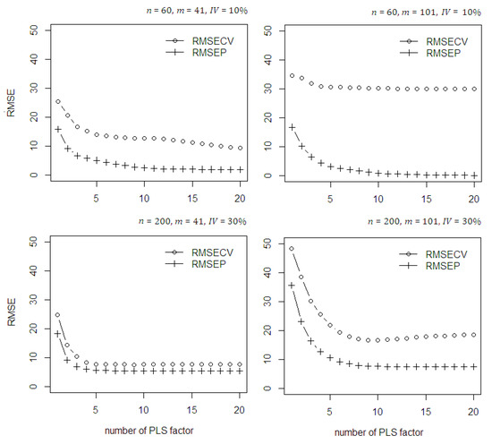
Figure 1. The RMSECV and RMSEP of the classical PLSR on the simulated data with no contamination of outlier and high leverage points.

The stability of the classical PLSR model then is evaluated by introducing the presence of outlier and leverage points in the dataset (see Figure 2). According to the scenarios given, the classical PLSR model failed to converge even using higher number of PLS components. This can be investigated through RMSECV values which become large and fail to be minimum. In addition, the discrepancy between both RMSECV and RMSEP values also large. This gives evidence that the presence of outlier and HLP in the dataset will destroy the convergence and results to the poor model fitting.

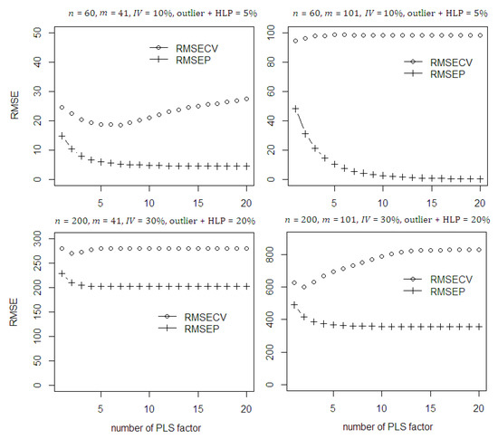
Figure 2. The RMSECV and RMSEP of the classical PLSR on the simulated data with contamination of outlier and high leverage points.

In the proposed RRWA-PLS, the 20% trimmed SEP was used to calculate the weight by removing the 20% highest absolute residual. This procedure is suggested to produce the robust weight instead of using the whole residual. In the calculation of trimmed SEP in each PLS component, using the cross validation procedure the median is preferred. In general, using different dataset scenarios with contamination of outlier and HLP (see Figure 3) the proposed robust trimmed SEP median succeed to remove the influence by removing 20% highest absolute residual. The SEP mean is suffered both with small ($n$ = 60) and bigger ($n$ = 200) sample size due to the contamination. This results in the SEP values of SEP mean becomes two to four times greater than trimmed SEP median. The SEP median lost its advantage when bigger sample size ($n$ = 200) is used. This results in the SEP values of SEP median becomes four times greater than trimmed SEP median. The SEP values using trimmed SEP median is lower than trimmed SEP mean thus improves model accuracy. This proves the robustness of the trimmed SEP median in weight calculation which irrespective of sample size, number of important variables, and percentage of contamination of outlier and HLP in the dataset.

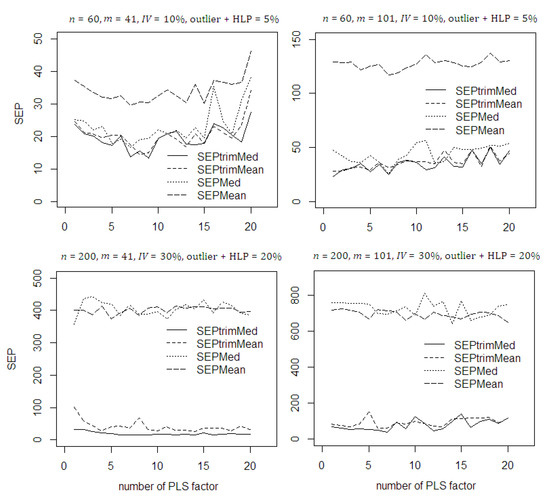
Figure 3. SEP values in the RRWA-PLS using different approach on the simulated data with contamination of outlier and HLP.

It is very important to compare the weighting schemes between the WA-PLS and RRWA-PLS. This weight provides the contribution of predictors based on the aggregation of the PLS components used in the model. In Figure 4, the mean weights of the methods are also shown to illustrate two conditions: no contamination and with contamination of outlier and high leverage points. For no contamination, the weights in both WA-PLS and RRWA-PLS methods increase as the number of PLS component increases. The weight of RRWA-PLS is relatively smaller than that of the WA-PLS. In cases where the number of PLS components are greater than 10, the weight in both methods are not so much affected by the increasing number of PLS used in the model. On the other hand, when contaminated with outlier and HLP, the weights in both WA-PLS and RRWA-PLS methods decrease as the number of PLS component increases. Based on these scenarios, the WA-PLS still produces higher RMSE than RRWA-PLS. In general, according to the less weight value used in the model, the RRWA-PLS method is still superior and more efficient than the WA-PLS.

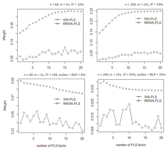
Figure 4. The mean weights of the WA-PLS and RRWA-PLS on the simulated data with and without contamination of outlier and HLP.

In Figure 5, the prediction accuracy of the methods is evaluated through their RMSEP values. To get a better illustration, the maximum number of PLS components was limited to 15 components. With no contamination of outlier and HLP in the dataset, in the first 6 number of PLS components, the RRWA-PLS is less efficient than the classical PLS and WA-PLS. However, as the number of PLS component increases up to 15, the RRWA-PLS is comparable to the classical PLS and WA-PLS. The proposed RRWA-PLS shows its robustness when the contaminations of outlier and HLP exist in the dataset. It has succeeded to prevent the influence of the outlier and HLP during model fitting. On the other hand, the classical PLS and WA-PLS suffer from the influence of outlier and HLP both in low and high level percentage of contamination, resulting in poor accuracy.

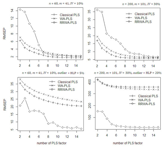
Figure 5. The RMSEP values of the classical PLS, WA-PLS, and RRWA-PLS on the simulated data with and without contamination of outlier and HLP.

To further evaluate the methods, the Monte Carlo simulation was run 10,000 times on different dataset scenarios. The results, based on the average of statistical measures, are shown in Table 1. As mentioned earlier, in the fitting process, the number of PLS components used in the proposed methods was limited to 15. We use the term “PLS with opt.” to refer to the classical PLS with optimal number of PLS component selected through the “onesigma” approach and cross-validation. We also include a weight improvement procedure in the WA-PLS known as MWA-PLS. The MWA-PLS uses the robust weight version in the RRWA-PLS to replace the non-robust weight in WA-PLS. Based on the results, with no outliers and HLP in the dataset, the non-robust PLSR coupled with optimal components and WA-PLS are comparable to the MWA-PLS and RRWA-PLS. On the other hand, in the presence of outliers and HLP, the proposed RRWA-PLS method is superior to the classical PLS, WA-PLS, and MWA-PLS. Replacing the weight in the WA-PLS with the weight of the robust version improves the model accuracy with lower SE and better R² values. The classical PLS fails to find the optimal number of PLS components due to the influence of 5–10% contamination of outliers and HLP during the fitting process. The WA-PLS also fails to fit the predicted model due to the impact of the contamination. The proposed RRWA-PLS consistently has the lowest RMSE, SE, and better R² compared to the other methods, irrespective of the sample sizes, number of important variables, and percentages of contamination of outliers and HLP in the dataset.

Table 1. The RMSE, R², and SE in the weighted methods using the Monte Carlo Simulation with different dataset scenarios.

Outlier and HLP	n	m	IV	Methods	nPLS	RMSE	R2	SE
No outlier and HLP	60	41	10%	PLS with opt.	9	2.752	0.980	2.776
				WA-PLS	15	2.496	0.984	2.517
				MWA-PLS	15	3.318	0.972	3.305
				RRWA-PLS	15	2.495	0.983	2.497
	60	101	10%	PLS with opt.	3	9.348	0.903	9.427
				WA-PLS	15	2.759	0.993	2.782
				MWA-PLS	15	8.181	0.931	8.250
				RRWA-PLS	15	2.702	0.960	2.708
	60	201	10%	PLS with opt.	1	18.717	0.859	18.875
				WA-PLS	15	2.333	0.998	2.352
				MWA-PLS	15	5.542	0.908	5.543
				RRWA-PLS	15	2.460	0.984	2.480
	200	41	30%	PLS with opt.	6	6.707	0.969	6.723
				WA-PLS	15	6.532	0.970	6.548
				MWA-PLS	15	6.799	0.968	6.816
				RRWA-PLS	15	6.594	0.970	6.610
	200	101	30%	PLS with opt.	10	7.926	0.980	7.946
				WA-PLS	15	7.915	0.981	7.935
				MWA-PLS	15	12.621	0.951	12.653
				RRWA-PLS	15	7.860	0.988	7.862
	200	201	30%	PLS with opt.	9	12.995	0.973	13.028
				WA-PLS	15	9.237	0.988	9.260
				MWA-PLS	15	15.163	0.965	15.201
				RRWA-PLS	15	9.582	0.985	9.601
	400	41	50%	PLS with opt.	4	9.213	0.967	9.224
				WA-PLS	15	9.062	0.968	9.073
				MWA-PLS	15	9.522	0.965	9.534
				RRWA-PLS	15	9.108	0.968	9.109
	400	101	50%	PLS with opt.	7	12.727	0.972	12.733
				WA-PLS	15	12.611	0.973	12.627
				MWA-PLS	15	18.812	0.939	18.836
				RRWA-PLS	15	12.787	0.972	12.803
	400	201	50%	PLS with opt.	10	14.244	0.981	14.262
				WA-PLS	15	14.343	0.981	14.361
				MWA-PLS	15	31.060	0.910	31.099
				RRWA-PLS	15	14.153	0.983	14.172
With outlier and HLP (5%)	60	41	10%	PLS with opt.	0	N/A	N/A	N/A
				WA-PLS	15	24.139	0.869	24.343
				MWA-PLS	15	3.160	0.975	3.188
				RRWA-PLS	15	3.042	0.976	3.069
	60	101	10%	PLS with opt.	0	N/A	N/A	N/A
				WA-PLS	15	16.559	0.892	16.699
				MWA-PLS	15	9.156	0.931	9.241
				RRWA-PLS	15	5.068	0.984	5.116
	60	201	10%	PLS with opt.	0	N/A	N/A	N/A
				WA-PLS	15	15.156	0.998	15.284
				MWA-PLS	15	9.500	0.936	9.591
				RRWA-PLS	15	8.580	0.973	8.662
	200	41	30%	PLS with opt.	1	151.317	0.494	151.697
				WA-PLS	15	175.959	0.603	176.400
				MWA-PLS	15	6.441	0.970	6.458
				RRWA-PLS	15	6.267	0.971	6.284
	200	101	30%	PLS with opt.	2	331.650	0.734	332.482
				WA-PLS	15	258.614	0.835	259.263
				MWA-PLS	15	10.679	0.960	10.707
				RRWA-PLS	15	8.195	0.976	8.217
	200	201	30%	PLS with opt.	1	462.150	0.855	462.307
				WA-PLS	15	226.599	0.969	227.167
				MWA-PLS	15	17.791	0.952	17.839
				RRWA-PLS	15	11.602	0.979	11.634
	400	41	50%	PLS with opt.	2	304.843	0.516	305.225
				WA-PLS	15	336.519	0.533	336.941
				MWA-PLS	15	8.841	0.964	8.853
				RRWA-PLS	15	8.383	0.968	8.394
	400	101	50%	PLS with opt.	2	569.727	0.718	570.441
				WA-PLS	15	537.184	0.776	537.857
				MWA-PLS	15	17.678	0.941	17.702
				RRWA-PLS	15	12.664	0.970	12.681
	400	201	50%	PLS with opt.	2	808.964	0.836	809.977
				WA-PLS	15	620.385	0.899	621.161
				MWA-PLS	15	29.338	0.920	29.377
				RRWA-PLS	15	17.163	0.973	17.186
With outlier and HLP (20%)	60	41	10%	PLS with opt.	2	94.896	0.718	95.697
				WA-PLS	15	72.625	0.903	73.238
				MWA-PLS	15	9.731	0.878	9.825
				RRWA-PLS	15	8.689	0.897	8.774
	60	101	10%	PLS with opt.	2	121.598	0.872	122.624
				WA-PLS	15	29.488	0.905	29.737
				MWA-PLS	15	12.795	0.932	12.924
				RRWA-PLS	15	10.488	0.934	10.596
	60	201	10%	PLS with opt.	2	209.076	0.721	210.841
				WA-PLS	15	26.243	0.899	26.464
				MWA-PLS	15	27.206	0.791	27.496
				RRWA-PLS	15	25.145	0.878	25.204
	200	41	30%	PLS with opt.	1	254.290	0.719	254.928
				WA-PLS	15	237.919	0.783	238.516
				MWA-PLS	15	7.848	0.956	7.872
				RRWA-PLS	15	7.383	0.961	7.406
	200	101	30%	PLS with opt.	1	438.504	0.855	439.604
				WA-PLS	15	353.163	0.928	354.049
				MWA-PLS	15	16.810	0.911	16.863
				RRWA-PLS	15	16.105	0.924	16.155
	200	201	30%	PLS with opt.	2	692.302	0.792	693.037
				WA-PLS	15	294.979	0.799	295.719
				MWA-PLS	15	121.881	0.740	122.262
				RRWA-PLS	15	34.982	0.891	35.091
	400	41	50%	PLS with opt.	1	443.979	0.740	444.535
				WA-PLS	15	396.425	0.767	396.921
				MWA-PLS	15	10.339	0.957	10.356
				RRWA-PLS	15	10.059	0.958	10.074
	400	101	50%	PLS with opt.	1	773.558	0.865	774.527
				WA-PLS	15	655.858	0.903	656.679
				MWA-PLS	15	23.244	0.912	23.281
				RRWA-PLS	15	23.066	0.913	23.102
	400	201	50%	PLS with opt.	1	944.986	0.792	945.425
				WA-PLS	15	803.520	0.796	804.526
				MWA-PLS	15	40.656	0.859	40.720
				RRWA-PLS	15	35.121	0.894	35.176

Note: nPLS is the number of optimal PLS components used in the PLSR model; PLS with opt. is the classical PLS with optimal number of PLS components.

The prediction ability of the methods using the contamination data was evaluated by plotting the predicted values against the actual values (see Figure 6). The classical PLS and WA-PLS suffered from the contamination of outliers and HLP in the dataset, which resulted in a poor prediction. This is because the PLSR estimator is not resistant to the contamination hence, biasing the estimated model. The MWA-PLS and proposed RRWA-PLS are completely free from the impact of outliers and HLP in the dataset. The influential observations are removed far from the fitting line, while good observations are closed to the fitted regression line. The prediction ability in RRWA-PLS is better than the MWA-PLS; the method ensures the best prediction capabilities with better accuracy than the other methods. The RRWA-PLS shows its robustness which is not affected by the inclusion of model with the number of PLS component used and is resistant to the influence of outliers and HLP.

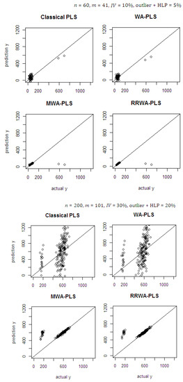
Figure 6. Predicted against actual values on the simulated data using PLS with opt., WA-PLS, MWA-PLS, and RRWA-PLS.

5. NIR Spectral Dataset

NIR spectral data from oil palm fruit mesocarp were collected to evaluate the methods. The spectral data use light absorbance in each $j$ wavelength bands adopted from Beer-Lambert Law [6], and the data are presented in $m\times 1$ column vector $x_j$ using the log base 10. The spectral measurement was performed by scanning (in contact) the fruit mesocarp using a Portable Handheld NIR spectrometer, QualitySpec Trek, from Analytical Spectral Devices (ASD Inc., Boulder, Colorado (CO), USA). A total of 80 fruit bunches were harvested from the site of breeding trial in Palapa Estate, PT. Ivomas Tunggal, Riau Province, Indonesia. There were 12 fruit mesocarp samples in a bunch collected from different sampling positions. The sampling positions comprised the vertical and horizontal lines in a bunch (see [23]): bottom-front, bottom-left, bottom-back, bottom-right, equator-front, equator-left, equator-back, equator-right, top-front, top-left, top-back, and top-right. Right after collection, the fruit mesocarp samples were sent immediately to the laboratory for spectral measurement and wet chemistry analysis. The source of variability such as planting materials (Dami Mas, Clone, Benin, Cameroon, Angola, Colombia), planting year (2010, 2011, 2012) and ripeness level (unripe, under ripe, ripe, over ripe) were also considered to cover the different sources of variation in the palm population as much as possible.

Two sets of NIR spectral data with different sample properties, the fresh fruit mesocarp and dried ground mesocarp, were used in the study. The average of three spectra measurement on each fruit sample mesocarp was used in the computation. The fresh fruit mesocarp was used to estimate the percentage of Oil to Dry Mesocarp (%ODM) and percentage of Oil to Wet Mesocarp (%OWM), while the dried ground mesocarp was used to estimate the percentage of Fat Fatty Acids (%FFA). These parameters were analyzed through conventional analytical chemistry that adopts standard test methods from the Palm Oil Research Institute of Malaysia (PORIM) [45,46]. The %ODM was calculated in dry matter basis, which removes the weight of water content, while the %OWM used wet matter basis. Statistically, the distribution range of %ODM used as dataset is 56.38–86.9%; the %OWM is 19.75–64.81%, and the %FFA is 0.17–6.3%. The NIR spectra on oil palm fruit mesocarp (both in fresh and dried ground mesocarp) and its frequency distribution on response variables, the %ODM, %OWM, and %FFA, can be seen in the previous study (see [23]). It is important to note that no prior knowledge on whether or not outliers and high leverage points are present in this dataset. The discussions were therefore, addressed to evaluate the methods based on their accuracy improvement through its desirability index.

5.1. Oil to Dry Mesocarp

A total of 960 observations which comprised 488 wavelengths (range 550–2500 nm: 4 nm interval) of NIR spectral of fresh fruit mesocarp were used in this study. Following a prior procedure, the cross validation scheme was employed to obtain the RMSECV value in parallel to the increasing number of PLS components. To evaluate the RMSE values both in fitting and prediction ability performance, the scree plot is presented in Figure 7. This plot is essential to observe when the slope starts leveling off and illustrate the gap difference between the RMSECV and RMSEP values. The maximum number of PLS components was limited to 30 for computation efficiency purpose.

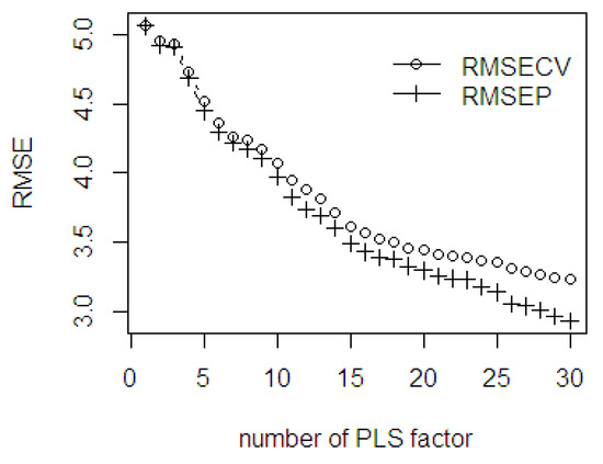
Figure 7. The RMSE of the fitted PLSR through cross validation and the prediction ability using %ODM dataset.

As seen in Figure 7, the stages of where the slope starts leveling off are at 7, 16, and 26 PLS components. The gap difference between the RMSECV and RMSEP values is wider after 26 PLS components, but both errors gradually become smaller. A larger discrepancy between the values indicates an over fitted which decreases the model accuracy. This indicates that despite using higher components, improvement in the accuracy is not guaranteed.

The mean weights of the fitted PLS both using WA-PLS and RRWA-PLS are plotted in Figure 8. It can be seen that the weight of the WA-PLS rapidly increases as the number of PLS components increases. This shows that using a higher number of PLS components improves accuracy. In RRWA-PLS, the weights are relatively comparable as the PLS components increases. It is interesting to observe that by using the weight strategy in RRWA-PLS, some components show lower mean weights compared to the others even though they have less and higher PLS components. For instance, applying 2 and 5 PLS components results in the signal for under fitting while applying 35 and 45 PLS components results in over fitting. The weighting scheme in the WA-PLS and RRWA-PLS depends on the number of PLS components used in the PLSR model. In fact, using a higher number of PLS components may risk in the inclusion of more noise, yielding a larger variation in the predicted model. The WA-PLS is known to be only suitable in preventing a large regression coefficient which indicates an over fitting. Through its corrected weights using reliability values, the RRWA-PLS does not only prevent over fitting but also under fitting.

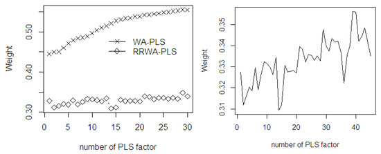
Figure 8. The mean weights of the fitted PLSR in WA-PLS and RRWA-PLS methods using %ODM dataset.

As seen in Figure 9, the prediction ability error between the classical PLS, WA-PLS, and RRWA-PLS are comparable to each other. The first minimal RMSEP was obtained with 7 PLS components. After the 7 PLS components, the WA-PLS produced a higher RMSEP than the classical PLS and RRWA-PLS. The second minimal RMSEP was obtained with 16 PLS components, and the third minimal RMSEP was obtained with 26 PLS components. The classical PLS and RRWA-PLS have similar prediction ability error with 4, 9, 27, 28, 29, and 30 PLS components used in the PLSR model. In general, the RMSEP values using RRWA-PLS method are always within the range and fall around the classical PLS. The RMSEP curve decreases slightly up to 30 PLS components. In an industrial application, the number of factor greater than 30 PLS components is not recommended. Although this would yield better prediction ability, it is computationally intensive.

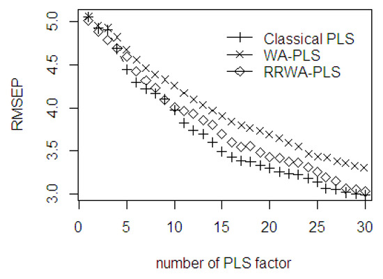
Figure 9. The RMSEP values of classical PLS, WA-PLS, RRWA-PLS method using %ODM dataset.

The performance of WA-PLS is not better than its modified weight in MWA-PLS (see Table 2). However, the accuracy of MWA-PLS is still lower than that of the RRWA-PLS. This is due to the weight in the WA-PLS which is not able to capture the reliability of the predictor variables. Comparing the prediction ability in the classical PLS with optimum PLS component (27), the RRWA-PLS is still superior. To prevent the influence of noise to the final model, we eliminated the first PLS component from the RRWA-PLS model. This is due to the fact that the first PLS component is usually less accurate if it is still included in the procedure.

Table 2. The RMSE, R², and SE in the weighted methods using %ODM data.

Dataset	Methods	nPLS	RMSEP	R2	SE
%ODM	PLS with opt.	27	3.139	0.648	3.141
	WA-PLS	30	3.316	0.603	3.317
	MWA-PLS	30	3.315	0.644	3.317
	RRWA-PLS	30	3.071	0.661	3.072

Note: nPLS is the number of optimal PLS components used in the PLSR model; PLS with opt. is the classical PLS with optimal number of PLS components.

5.2. Oil to Wet Mesocarp

In this section, the %OWM is considered as the response variable of the NIR spectral fresh fruit mesocarp dataset. The evaluation on the RMSE values, both in fitting and prediction ability, is presented in the scree plot. The maximum number of PLS components was limited to 30 for computation efficiency purposes. As seen in Figure 10, the slope of scree plot starts leveling off at 7, 16, and 22 PLS components. The gap difference between the RMSECV and RMSEP values are wider after the 22 PLS components. Contrarily, even though both errors become slightly smaller, a large difference between the RMSECV and RMSEP would lead to over fitting and make the predicted model unstable.

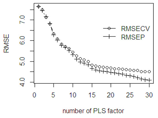
Figure 10. The RMSE of the fitted PLSR through cross validation and the prediction ability using %OWM dataset.

With the increasing number of PLS components, the mean weights of both WA-PLS and RRWA-PLS also increase (see Figure 11). The mean weights of WA-PLS method are comparably higher to the weight in the RRWA-PLS where accuracy is improved by employing a higher number of PLS components. There are some components in the RRWA-PLS with mean weights lower than those of other PLS components although they have a higher number of components. Applying 2 and 5 PLS components results under fitting, while applying 26 and 29 PLS components results in over fitting. The RRWA-PLS shows its robustness which is not dependent on the increasing number of PLS components used. Its weighing scheme is based on the selection of the relevant aggregate number of PLS components used as factors in the PLSR model. The most relevant PLS components will get a higher weight, while the less relevant will obtain a lower weight.

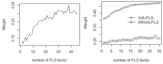
Figure 11. The mean weights of the fitted PLSR in WA-PLS and RRWA-PLS methods using %OWM dataset.

Figure 12 indicates that the prediction ability of the three methods using the first 5 components is fairly close to each other, but afterwards their performances seem to be different in terms of accuracy. The first minimal RMSEP is obtained with 8 PLS components. After the 8 PLS components, the WA-PLS produces higher RMSEP than the classical PLS and RRWA-PLS. The second minimal RMSEP is obtained with 14 PLS components, and the third minimal RMSEP is obtained with 23 PLS components. The classical PLS with 15 to 22 PLS components produces lower RMSEP values; however, after 24 PLS components, the accuracy between RRWA-PLS and classical PLS becomes closer. In general, the RMSEP values using RRWA-PLS method are always within the range, and the values are reasonably close to the classical PLS. The RMSEP curves slightly decrease which begin from 17 to 30 PLS components. The WA-PLS relatively has low accuracy compared to the RRWA-PLS and classical PLS. The WA-PLS suffers from over-under fitting due to several irrelevant variables, but it may still possibly be included in the fitting process.

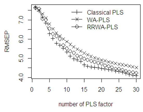
Figure 12. The RMSEP values of classical PLS, WA-PLS, RRWA-PLS method using %OWM dataset.

Using its optimum at 22 PLS components, the classical PLS with the optimum number of PLS components is indeed inconsistent and sensitive to the number of PLS components used. By comparing the RMSE, R², and SE values in Table 3, it can be concluded that the proposed RRWA-PLS produces better accuracy than the other methods. The modified weight in MWA-PLS has improved the accuracy of the predicted model; however, it cannot outperform the RRWA-PLS. The robust weighted-average strategy prevents the PLSR model from depending on the specific number of PLS components used in the fitting process.

Table 3. The RMSE, R², and SE in the weighted methods using %OWM data.

Dataset	Methods	nPLS	RMSEP	R2	SE
%OWM	PLS with opt.	22	4.442	0.668	4.444
	WA-PLS	30	4.520	0.672	4.522
	MWA-PLS	30	4.239	0.708	4.241
	RRWA-PLS	30	4.185	0.718	4.187

Note: nPLS is the number of optimal PLS components used in the PLSR model; PLS with opt. is the classical PLS with optimal number of PLS components.

5.3. Fat Fatty Acids

The NIR spectral of dried ground mesocarp with a total of 839 observations and 500 wavelengths (range 500–2500 nm: 4 nm interval) were utilized as predictor variables. Here, the %FFA was used as the response variable. In the scree plot (Figure 13), the RMSECV and RMSEP curves gradually decrease when the number of PLS components increases. Within the first 10 PLS components, the gap difference between RMSECV and RMSEP is small, but after 10 PLS components, the gap difference starts to increase continuously. The slope of the scree plot starts leveling off at the 6, 16, 22, and 27 PLS components. The gap difference between the RMSECV and RMSEP values becomes wider after 16 PLS components. Therefore, the use of specific number of PLS components affects the accuracy of the fitted model.

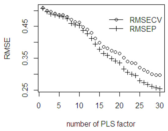
Figure 13. The RMSE of the fitted PLSR through cross validation and the prediction ability using %FFA dataset.

The mean weights of both WA-PLS and RRWA-PLS increase as the number of PLS component (see Figure 14) increases. Using %FFA dataset, the weight of RRWA-PLS is higher than that of the WA-PLS. The mean weights of the WA-PLS method increase more steeply as the number of PLS components increases. This indicates that the predicted model tends to be over fitting. The weight of the RRWA-PLS is robust since its weight does not depend on the aggregation number of PLS components used, irrespective of the number of sample size and the number of important variables. Moreover, the weight is resistant to the influence of outliers and HLP that may exist in the dataset.

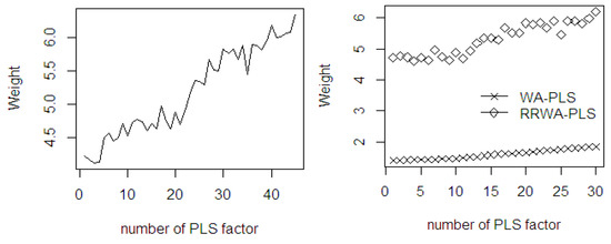
Figure 14. The mean weights of the fitted PLSR in WA-PLS and RRWA-PLS methods using %FFA dataset.

In the first 6 components, the prediction ability of the three methods is comparable to each other (see Figure 15). After 10 components, the WA-PLS has less accuracy than the classical PLS and the RRWA-PLS. The first minimal RMSEP is obtained at 8 PLS components; after 8 PLS components, the WA-PLS produces larger RMSEP than the classical PLS and the RRWA-PLS. The WA-PLS shows the worst performance using this %FFA dataset. The second minimal RMSEP is obtained at 17 PLS components, and the third minimal RMSEP is obtained at 27 PLS components. The RMSEP values using RRWA-PLS method are always within the range and close to the classical PLS. The RMSEP in the classical PLS is not robust when it comes to the number of PLS components used as using any selection methods to find the optimal number of PLS components to be used in the PLSR model will result in unstable results. The application of an improper method in the selection will produce a less accurate result. The solution in using the robust weighted average is then suggested as it is unnecessary to find the optimal components. This is the automated fitting process in the PLSR model.

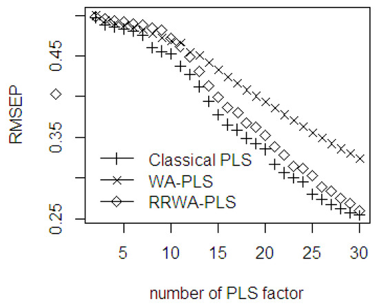
Figure 15. The RMSEP values of classical PLS, WA-PLS, RRWA-PLS method using %FFA dataset.

In Table 4, the classical PLS really suffers from the model complexity used in the fitting process. Using the one-sigma heuristic method in component selection, the accuracy of the selected optimal number of PLS components is not better than the PLS with a higher number of components. This shows the weakness of using a specific number of PLS components in the PLSR model. The robust RRWA-PLS is free from the complexity of the aggregation number of PLS components used. As seen in Table 3, the WA-PLS has the worst performance compared to the MWA-PLS, classical PLS, and RRWA-PLS. The use of RRWA-PLS method is preferred to the classical PLS because it does not require the selection of an optimal number of PLS components to be used in the final PLSR model. In addition, the method offers better reliability of the goodness-of-fit for the model.

Table 4. The RMSE, R², and SE in the weighted methods using %FFA data.

Dataset	Methods	nPLS	RMSEP	R2	SE
%FFA	PLS with opt.	27	0.287	0.729	0.288
	WA-PLS	30	0.324	0.658	0.324
	MWA-PLS	30	0.311	0.683	0.312
	RRWA-PLS	30	0.275	0.747	0.276

Note: nPLS is the number of optimal PLS components used in the PLSR model; PLS with opt. is the classical PLS with optimal number of PLS component.

6. Reliability Values

A number of irrelevant variables most probably still exist in the dataset. If the PLSR method fails to screen and downgrade the contribution of these irrelevant variables, it might decrease the accuracy of the final fitted model. The use of RRWA-PLS on the artificial dataset (see Figure 16a) helps the method to screen the most relevant variables and downgrade the irrelevant variables in the dataset successfully. The use of NIR spectral data with different response variables (%ODM, %OWM, and %FFA) has allowed the method to show its potential in the wavelength selection process. The method highlights the most relevant wavelengths and downgrades the influence of irrelevant wavelengths based on spectra absorption (see Figure 16b–d). The reliability values are important in order to increase the computational speed in the fitting process, improve the accuracy, and provide better interpretation of the NIR spectral dataset.

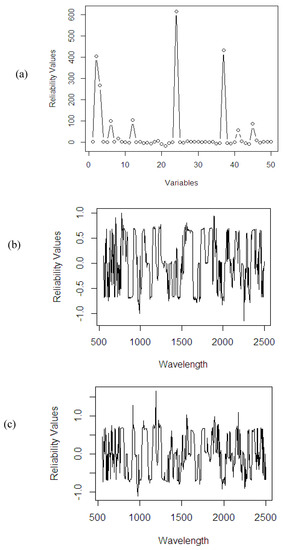
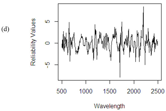
Figure 16. Reliability values using RRWA-PLS method on different datasets: (a) artificial data; NIR spectral dataset: (b) %ODM; (c) %OWM; (d) %FFA.

7. Conclusions

This study has shown the robustness in the chemometric analysis of NIR spectral data related to the aggregate number of PLS components and the resistance against outliers and HLP. The rich and abundant information in the NIR spectral requires advanced chemometric analysis to classify the most and least relevant wavelengths used in computation. Based on the results, the proposed RRWA-PLS method is the most preferred method compared to other methods due to its robustness. The weight improvement in MWA-PLS gives a better solution in improving the accuracy and reliability of WA-PLS. In the selection of the optimal number of PLS components, the classical PLS still needs the re-computational process to determine a specific complexity each time the model is updated. The proposed RRWA-PLS shows its superiority in the improvement of weight and variable selection process. It is also resistant to the contamination of outliers and HLP in the dataset. In addition, the RRWA-PLS method offers a solution for automated fitting process in the PLSR model as it does not require the selection of the optimal number of PLS components unlike in the classical PLS.

References

- Rodriguez-Saona, L.E.; Fry, F.S.; McLaughlin, M.A.; Calvey, E.M. Rapid analysis of sugars in fruit juices by FT-NIR spectroscopy. Carbohydr. Res. 2001, 336, 63–74. [Google Scholar] [CrossRef]
- Blanco, M.; Villarroya, I.N.I.R. NIR spectroscopy: A rapid-response analytical tool. Trends Anal. Chem. 2002, 21, 240–250. [Google Scholar] [CrossRef]
- Alander, J.T.; Bochko, V.; Martinkauppi, B.; Saranwong, S.; Mantere, T. A review of optical nondestructive visual and near-infrared methods for food quality and safety. Int. J. Spectrosc. 2013, 2013, 341402. [Google Scholar] [CrossRef]
- Lee, C.; Polari, J.J.; Kramer, K.E.; Wang, S.C. Near-Infrared (NIR) Spectrometry as a Fast and Reliable Tool for Fat and Moisture Analyses in Olives. ACS Omega. 2018, 3, 16081–16088. [Google Scholar] [CrossRef] [PubMed]
- Levasseur-Garcia, C. Updated overview of infrared spectroscopy methods for detecting mycotoxins on cereals (corn, wheat, and barley). Toxins 2018, 10, 38. [Google Scholar] [CrossRef]
- Stuart, B. Infrared Spectroscopy: Fundamentals and Applications; Wiley: Toronto, ON, Canada, 2004; pp. 167–185. [Google Scholar]
- Mark, H. Chemometrics in near-infrared spectroscopy. Anal. Chim. Acta 1989, 223, 75–93. [Google Scholar] [CrossRef]
- Cozzolino, D.; Morón, A. Potential of near-infrared reflectance spectroscopy and chemometrics to predict soil organic carbon fractions. Soil Tillage Res. 2006, 85, 78–85. [Google Scholar] [CrossRef]
- Roggo, Y.; Chalus, P.; Maurer, L.; Lema-Martinez, C.; Edmond, A.; Jent, N. A review of near infrared spectroscopy and chemometrics in pharmaceutical technologies. J. Pharm. Biomed. Anal. 2007, 44, 683–700. [Google Scholar] [CrossRef]
- Garthwaite, P.H. An interpretation of partial least squares. J. Am. Stat. Assoc. 1994, 89, 122–127. [Google Scholar] [CrossRef]
- Cozzolino, D.; Kwiatkowski, M.J.; Dambergs, R.G.; Cynkar, W.U.; Janik, L.J.; Skouroumounis, G.; Gishen, M. Analysis of elements in wine using near infrared spectroscopy and partial least squares regression. Talanta 2008, 74, 711–716. [Google Scholar] [CrossRef]
- McLeod, G.; Clelland, K.; Tapp, H.; Kemsley, E.K.; Wilson, R.H.; Poulter, G.; Coombs, D.; Hewitt, C.J. A comparison of variate pre-selection methods for use in partial least squares regression: A case study on NIR spectroscopy applied to monitoring beer fermentation. J. Food Eng. 2009, 90, 300–307. [Google Scholar] [CrossRef]
- Xu, L.; Cai, C.B.; Deng, D.H. Multivariate quality control solved by one-class partial least squares regression: Identification of adulterated peanut oils by mid-infrared spectroscopy. J. Chemom. 2011, 25, 568–574. [Google Scholar] [CrossRef]
- Wold, H. Model construction and evaluation when theoretical knowledge is scarce: Theory and application of partial least squares. In Evaluation of Econometric Models; Elsevier: Amsterdam, The Netherlands, 1980; pp. 47–74. [Google Scholar]
- Manne, R. Analysis of two partial-least-squares algorithms for multivariate calibration. Chemom. Intell. Lab. Syst. 1987, 2, 187–197. [Google Scholar] [CrossRef]
- Haenlein, M.; Kaplan, A.M. A beginner’s guide to partial least squares analysis. Understt. Satistics 2004, 3, 283–297. [Google Scholar] [CrossRef]
- Hubert, M.; Branden, K.V. Robust methods for partial least squares regression. J. Chemom. A J. Chemom. Soc. 2003, 17, 537–549. [Google Scholar] [CrossRef]
- Silalahi, D.D.; Midi, H.; Arasan, J.; Mustafa, M.S.; Caliman, J.P. Robust generalized multiplicative scatter correction algorithm on pretreatment of near infrared spectral data. Vib. Spectrosc. 2018, 97, 55–65. [Google Scholar] [CrossRef]
- Rosipal, R.; Trejo, L.J. Kernel partial least squares regression in reproducing kernel hilbert space. J. Mach. Learn. Res. 2001, 2, 97–123. [Google Scholar]
- Silalahi, D.D.; Midi, H.; Arasan, J.; Mustafa, M.S.; Caliman, J.P. Kernel partial diagnostic robust potential to handle high-dimensional and irregular data space on near infrared spectral data. Heliyon 2020, 6, e03176. [Google Scholar] [CrossRef]
- Centner, V.; Massart, D.L.; De Noord, O.E.; De Jong, S.; Vandeginste, B.M.; Sterna, C. Elimination of uninformative variables for multivariate calibration. Anal. Chem. 1996, 68, 3851–3858. [Google Scholar] [CrossRef]
- Mehmood, T.; Liland, K.H.; Snipen, L.; Sæbø, S. A review of variable selection methods in partial least squares regression. Chemom. Intell. Lab. Syst. 2012, 118, 62–69. [Google Scholar] [CrossRef]
- Silalahi, D.D.; Midi, H.; Arasan, J.; Mustafa, M.S.; Caliman, J.P. Robust Wavelength Selection Using Filter-Wrapper Method and Input Scaling on Near Infrared Spectral Data. Sensors 2020, 20, 5001. [Google Scholar] [CrossRef] [PubMed]
- Wiklund, S.; Nilsson, D.; Eriksson, L.; Sjöström, M.; Wold, S.; Faber, K. A randomization test for PLS component selection. J. Chemom. A J. Chemom. Soc. 2007, 21, 427–439. [Google Scholar] [CrossRef]
- Hastie, T.; Tibshirani, R.; Friedman, J. The elements of statistical learning: Data mining, inference, and prediction. In Springer Series in Statistics; Springer: Berlin/Heidelberg, Germany, 2009. [Google Scholar]
- Van Der Voet, H. Comparing the predictive accuracy of models using a simple randomization test. Chemom. Intell. Lab. Syst. 1994, 25, 313–323. [Google Scholar] [CrossRef]
- Efron, B. Bootstrap Methods: Another Look at the Jackknife. Annal. Stat. 1979, 7, 1–26. [Google Scholar] [CrossRef]
- Gómez-Carracedo, M.P.; Andrade, J.M.; Rutledge, D.N.; Faber, N.M. Selecting the optimum number of partial least squares components for the calibration of attenuated total reflectance-mid-infrared spectra of undesigned kerosene samples. Anal. Chim. Acta 2007, 585, 253–265. [Google Scholar] [CrossRef] [PubMed]
- Tran, T.; Szymańska, E.; Gerretzen, J.; Buydens, L.; Afanador, N.L.; Blanchet, L. Weight randomization test for the selection of the number of components in PLS models. J. Chemom. 2017, 31, e2887. [Google Scholar] [CrossRef]
- Kvalheim, O.M.; Arneberg, R.; Grung, B.; Rajalahti, T. Determination of optimum number of components in partial least squares regression from distributions of the root-mean-squared error obtained by Monte Carlo resampling. J. Chemom. 2018, 32, e2993. [Google Scholar] [CrossRef]
- Shenk, J.S.; Westerhaus, M.O.; Berzaghi, P. Investigation of a LOCAL calibration procedure for near infrared instruments. J. Near Infrared Spectrosc. 1997, 5, 223–232. [Google Scholar] [CrossRef]
- Barton, F.E.; Shenk, J.S.; Westerhaus, M.O.; Funk, D.B. The development of near infrared wheat quality models by locally weighted regressions. J. Near Infrared Spectrosc. 2000, 8, 201–208. [Google Scholar] [CrossRef]
- Naes, T.; Isaksson, T.; Kowalski, B. Locally weighted regression and scatter correction for near-infrared reflectance data. Anal. Chem. 1990, 62, 664–673. [Google Scholar] [CrossRef]
- Dardenne, P.; Sinnaeve, G.; Baeten, V. Multivariate calibration and chemometrics for near infrared spectroscopy: Which method? J. Near Infrared Spectrosc. 2000, 8, 229–237. [Google Scholar] [CrossRef]
- Zhang, M.H.; Xu, Q.S.; Massart, D.L. Averaged and weighted average partial least squares. Anal. Chim. Acta 2004, 504, 279–289. [Google Scholar] [CrossRef]
- Serneels, S.; Croux, C.; Filzmoser, P.; Van Espen, P.J. Partial robust M-regression. Chemom. Intell. Lab. Syst. 2005, 79, 55–64. [Google Scholar] [CrossRef]
- Cui, C.; Fearn, T. Comparison of partial least squares regression, least squares support vector machines, and Gaussian process regression for a near infrared calibration. J. Near Infrared Spectrosc. 2017, 25, 5–14. [Google Scholar] [CrossRef]
- Song, W.; Wang, H.; Maguire, P.; Nibouche, O. Local Partial Least Square classifier in high dimensionality classification. Neurocomputing 2017, 234, 126–136. [Google Scholar] [CrossRef]
- Martens, H.; Naes, T. Multivariate Calibration; John Wiley & Sons: Hoboken, NJ, USA, 1992. [Google Scholar]
- Huber, P.J. Robust regression: Asymptotics, conjectures and Monte Carlo. Ann. Stat. 1973, 1, 799–821. [Google Scholar] [CrossRef]
- Cummins, D.J.; Andrews, C.W. Iteratively reweighted partial least squares: A performance analysis by Monte Carlo simulation. J. Chemom. 1995, 9, 489–507. [Google Scholar] [CrossRef]
- Fushiki, T. Estimation of prediction error by using K-fold cross-validation. Stat. Comput. 2011, 21, 137–146. [Google Scholar] [CrossRef]
- Kim, S.; Okajima, R.; Kano, M.; Hasebe, S. Development of soft-sensor using locally weighted PLS with adaptive similarity measure. Chemom. Intell. Lab. Syst. 2013, 124, 43–49. [Google Scholar] [CrossRef]
- Minasny, B.; McBratney, A. Why you don’t need to use RPD. Pedometron 2013, 33, 14–15. [Google Scholar]
- Siew, W.L.; Tan, Y.A.; Tang, T.S. Methods of Test for Palm Oil and Palm Oil Products: Compiled; Lin, S.W., Sue, T.T., Ai, T.Y., Eds.; Palm Oil Research Institute of Malaysia: Selangor, Malaysia, 1995.
- Rao, V.; Soh, A.C.; Corley, R.H.V.; Lee, C.H.; Rajanaidu, N. Critical Reexamination of the Method of Bunch Quality Analysis in Oil Palm Breeding; PORIM Occasional Paper; FAO: Rome, Italy, 1983; Available online: https://agris.fao.org/agris-search/search.do?recordID=US201302543052 (accessed on 13 October 2020).
Publisher’s Note: MDPI stays neutral with regard to jurisdictional claims in published maps and institutional affiliations. |
© 2020 by the authors. Licensee MDPI, Basel, Switzerland. This article is an open access article distributed under the terms and conditions of the Creative Commons Attribution (CC BY) license (http://creativecommons.org/licenses/by/4.0/).