Genetic Similarity Analysis Based on Positive and Negative Sequence Patterns of DNA

Abstract

Similarity analysis of DNA sequences can clarify the homology between sequences and predict the structure of, and relationship between, them. At the same time, the frequent patterns of biological sequences explain not only the genetic characteristics of the organism, but they also serve as relevant markers for certain events of biological sequences. However, most of the aforementioned biological sequence similarity analysis methods are targeted at the entire sequential pattern, which ignores the missing gene fragment that may induce potential disease. The similarity analysis of such sequences containing a missing gene item is a blank. Consequently, some sequences with missing bases are ignored or not effectively analyzed. Thus, this paper presents a new method for DNA sequence similarity analysis. Using this method, we first mined not only positive sequential patterns, but also sequential patterns that were missing some of the base terms (collectively referred to as negative sequential patterns). Subsequently, we used these frequent patterns for similarity analysis on a two-dimensional plane. Several experiments were conducted in order to verify the effectiveness of this algorithm. The experimental results demonstrated that the algorithm can obtain various results through the selection of frequent sequential patterns and that accuracy and time efficiency was improved.

1. Introduction

In recent years, a large volume of biological sequence data has been generated. When a new DNA sequence is obtained, similarity analysis is used in order to determine whether it is similar to a known sequence. If it is homologous, this will save time and effort in re-determining the function of the new sequence. In bioinformatics research, similarity analysis of biological sequences is by no means a straightforward mechanical comparison. However, numerous mathematical and statistical methods are used to assist in analysis. In sequence similarity analysis, alignment and classical research methods are the most common. In sequence alignment, two problems exist that directly affect the similarity score: the substitution matrix and gap penalty. Gap penalty is used to compensate the influence of insertion and deletion on sequence similarity and no suitable theoretical model exists to describe the slot problem. Therefore, vacancy penalty points lack a functional theoretical basis and are subjectivity.

First, the drawbacks of sequence alignment have caused researchers to explore other methods for comparing DNA sequence similarities. For example, experts have devised various mathematical schemes. The graphical representation of biological sequences can identify the information content of any sequence to help biologists to choose another complex theoretical or experimental method. However, several problems still exist with these methods. For example, biological sequences often comprise thousands of base sequences and a large amount of time and storage space is consumed with mathematical representation and similarity analysis. Second, the aforementioned similarity analysis method can only produce a unique evolutionary relationship or distance matrix. Different methods will produce different analytical results, which greatly affect the accuracy and efficiency of analysis. In addition, existing similarity analysis methods are for positive sequential patterns (PSPs). For negative sequential patterns (NSPs), still no unified similarity measurement method exists. We know that the presence of NSPs in biological data is inevitable and is even crucial to some types of disease-causing genes. This motivated us to explore a method for performing similarity analysis of DNA with a missing base sequence. We will graphically represent the maximum frequent sequential patterns of a two-dimensional plane and then analyze the similarity with the represented DNA sequences.

Before performing similarity analysis, we need to perform sequential pattern mining on biological data. Mining NSPs is a difficult yet crucial task in DNA similarity analysis. Sequential pattern mining can locate all of the frequent sequential patterns in a given sequence database and it has been widely used in numerous fields [1,2,3], such as sequence classification and prediction, Web access pattern analysis, customer purchase pattern analysis, natural language sequence analysis, and biological sequence analysis. PSP mining only considers events (behaviors) that have already occurred, which is different from traditional sequential pattern mining. NSPs take into account events (behaviors) that have not yet occurred [4], which is, items not in the sequence that provide comprehensive information regarding human beings. Examples include the different degrees of impact on various existing situations in a student’s life [5] and a missing gene that may induce potential diseases, but that is ignored by humans. Similarity analysis of biological sequences also exists, which describes the evolutionary relationships between species. However, if a species has a missing gene that is treated as a normal gene, this can have a significant effect on the results of the analysis. It is more meaningful to study the sequence of missing base pairs than it is to find the sequential patterns of frequent sequences. The NSPs in this paper refer to a sequence containing a missing base.

In the past, PSP mining was at the center of biological sequential pattern mining. However, the progress of NSP mining research in recent years has been very limited, and most mining algorithms show low efficiency and high computational complexity. In 2011, our team proposed an e-NSP [6] algorithm. However, e-NSP time efficiency is not high and it consumes more storage space. Therefore, Dong further improved the e-NSP and proposed the f-NSP [7], which is based on bit operation, greatly improving the time and space efficiency of the algorithm. Accordingly, we apply the f-NSP frequent pattern mining of biological sequences, which can mine a large number of useful PSPs. Furthermore, this method can also mine a large volume of NSPs, for which efficiency is significantly improved, and the result of this mining is the data set for our subsequent work.

Not only does our method describe biological evolutionary relationships more accurately, but various pattern combinations can produce different results. The similarity analysis that we performed on the basis of frequent patterns caused the sequence length to be very short, which saved time and decreased space consumption. When compared with other methods, we also added similarity analysis for NSPs, which we proved experimentally.

The structure of this paper is as follows. Section 2 discusses the work that is related to the research objective. Section 3 provides the corresponding definitions and concepts of several specialized terms that are encountered in the research. Section 4 briefly introduces the relevant knowledge of f-NSP. Section 5, in detail, introduces the similarity analysis method and the process of negative biological sequencing. Section 6 demonstrates the research and experimentation on similarity analysis using real data that was performed and compared with other methods. We prove that the analysis performed with our method can make the results more accurate. Section 7 presents conclusions and future work.

2. Related Work

This section is divided into two parts: the first describes the pattern similarity analysis of biological sequences and the second describes the biological sequential pattern mining technique that we used.

2.1. Pattern Similarity Analysis of Biological Sequences

In recent decades, numerous DNA sequence similarity analysis methods have been proposed. At present, DNA similarity analysis [8,9] primarily focuses on elucidating a homologous relationship between sequence or predicting the structure and function of unidentified sequences in known sequences. The DNA sequence consists of four bases, adenine, thymine, cytosine, and guanine, which are represented by the letters A, T, C, and G, respectively. Most of the methods cannot process this sequence of letters, so we need to convert them into a sequence of numbers. Most DNA similarity analysis methods can also be divided into a graphic representation and other schemes according to their digital forms. Of these methods, graphic representation is a popular research field in DNA sequence similarity analysis. This method was first proposed by Hamori and Ruskin [10] and it has been subsequently widely used.

The graphics-based approach can be further divided into several categories that are based on the spatial dimension of the sequence, from two-dimensional (2-D) to three-dimensional (3-D), and other categories. The two-dimensional graphical representation of DNA sequences is a useful method for studying gene sequences [11]. The primary objective of representing nucleotides as digital vectors and mapping the DNA sequence in curves on a two-dimensional plane, based on the numerical characteristics of the DNA sequence that can be obtained. Gong et al. proposed new DNA sequence descriptors [12] that are derived from geometric concepts of curvature approximation and eigenvalue absence, which have the complexity of linear sequence length growth. Guo et al. proposed another similarity analysis method of DNA sequences that were built on two-dimensional graphical representation [13]. One DNA sequence corresponds to 24 different curves, which are organized in a two-dimensional Cartesian coordinate system. However, this ignores the chemical structure of the DNA sequence and omits most of its chemical information. In 2014, Ma et al. introduced a new type of iterative functional system in order to outline the two-dimensional graphical representation of protein sequences [14], which combines the various physic-chemical properties of amino acids. Lee et al. proposed a similarity measure that is capable of handling non-overlapped data and analyzed its characteristics on data distributions [15]. In order to obtain discriminative similarity values for non-overlapped data, Lee considered two approaches. The first was to adopt the traditional similarity measurement method after preprocessing the non-overlapping data. The second was to consider the neighbor data information when designing the similarity measure, where the relationship to specific data and residual data information was considered. In 2018, Xie et al. proposed the F-B curve and its corresponding single-base correlation 2D curve method [16]. The construction of these graphic curves is based on the allocation of individual bases of four different sine (or tangent) functions. In 2019, Abo-Elkhier et al. numerically represented each amino acid in the protein sequence and proposed a new 2-D graphical representation method [17]. They introduced a new descriptor that consisted of a vector $(\overline{A_t},S{A}_t)$ consisting of the mean and standard deviation from the total number of protein sequences. In addition, numerous 3-D methods also exist. For example, based on 64 codons and four nucleotide chemical DNA sequences, Jafarzadeh et al. proposed another 3-D representation method (C-Curve) [18]. However, this three-dimensional approach may require more storage space and pose a larger computational challenge than a 2-D approach. Numerous other types of graphical representations also exist, such as those that were proposed by Liao et al. [19]. According to the classification of the four bases of DNA, the main sequence is converted into a structure diagram. Invariants, such as topological index, were extracted from the graphical representation of these primary DNA sequences and then used to compute the similarity between the 11 species.

None of the above methods can effectively analyze the sequence of missing bases. Furthermore, in order to effectively analyze DNA sequence similarity, several key issues need to be considered: (1) how to effectively represent a DNA sequence with a digital sequence; (2) how to select appropriate descriptors that can be regarded as DNA sequence characteristics and then characterize them according to the digital sequence; and, (3) how to effectively process DNA sequences of various lengths and maintain their consistency. In this regard, we propose graphically representing the maximum frequent sequential patterns on a two-dimensional plane and analyzing the similarity with the represented DNA sequences.

2.2. Biological Sequential Pattern Mining Technique

In this section, we begin with PSP mining of biological sequences and then introduce NSP mining.

Biological sequential pattern mining is a major research topic for mining frequent sub-sequences in biological sequence databases as patterns and it has a wide range of application prospects, such as the early STAR algorithm [20]. Kurtz et al. proposed the REPuter algorithm that is based on the suffix tree [21], which overcomes the limitation of input sequence size, but with which is difficult to find repeat sequences with a high occurrence frequency of DNA sequences that are based on paired sub-sequences. Deng et al. [22] proposed a new method for frequent pattern mining in DNA sequences, which is based on two levels of nested hash table data structures and set operations. Scanning the DNA sequence one time reveals all frequent patterns and their positions in the DNA sequence. In 2018, Zhang proposed MulMer [23], which effectively mines all distinct multi-mers. MulMer first utilizes the inverted-index technique in order to project the original sequence and the method of pattern growth is then adopted to generate potential multi-mers; each multi-mers accurately records its location in the original sequence.

Few papers exist on NSP mining and none have applied NSP mining to DNA and protein sequences. We briefly introduce this below. Hsueh and colleagues designed an NSP mining method, named PNSP [24], which comprises three mining process steps. The first step is to use traditional algorithms to mine PSPs. The second step is to derive the negative item sets from the positive item sets. The third step is to join the positive and negative item sets to generate the positive and negative candidate sequential patterns using a method that is similar to prior concatenation. Finally, the candidate sequence support is obtained based on a database repeat scan, and the PSPs and NSPs are determined. Zheng et al. have introduced a GSP method in order to determine NSPs, referred to as Negative-GSP [25]. It first discovers PSPs through GSP after using a modified connection method and pruning operation in order to generate and trim a negative sequential candidate (NSC). The negative pattern is then generated by rescanning the database to calculate the support degree of the NSCs. Ouyang et al. proposed a discoverable from the NSP mining algorithm, such as $(\neg A,B)$, $(A,\neg B)$ and $(\neg A,\neg B)$. The pattern mining negative association rules are very close. This method needs to meet $(A\cap B)=\varphi$. The primary objective of this method is to obtain all frequent item sets, after the use of frequent item sets to generate frequent and infrequent sequences. The NSP is then mined from infrequent positive sequences. The work that was published in [26] raised the issue of NSPs, but did not provide a concrete solution; the work that was published in [27] used the same NSP as in the existing literature and applied it to an incremental database. Lin proposed an NSP mining algorithm, named NSPM [28]; however, the NSP defined in this algorithm only allows for the last element of the sequence to be a negative term and all other elements must be positive terms. Repetitive sequence patterns capture repetitions of sequence patterns in various sequences and understanding their behavior from the repeated relationship between them is crucial. Therefore, Dong et al. proposed a type of effective algorithm, called an e-RNSP [29], in order to mine the repetitions of NSPs (RNSPs). This method can convert repeated negative constraints to repeated positive constraints, and it can quickly calculate repetition supports by only using the corresponding RPSP information without rescanning the entire database. However, NSP mining is still in its infancy and it faces numerous challenging problems, one of which is how to select useful NSPs. In order to solve this first problem, Dong et al. proposed a Topk-NSP [30] algorithm to mine k of the most common negative patterns and, of these, the authors proposed three optimization strategies. Topk-NSP was the first algorithm that is capable of mining the most commonly used k NSPs. A fairly good e-NSP exists, but it has its drawbacks, which we will not describe here, because they were mentioned in the first section above. The f-NSP was selected to mine DNA sequences, which not only efficiently mined frequent sequential patterns, but also numerous NSPs, which are crucial for our next similarity analysis of DNA.

The current similarity analysis methods of biological sequences continue to be of interest to researchers. Numerous approaches have been proposed, but room for improvement still exists. In particular, no method exists for similarity analysis of NSPs. This paper proposes the adoption of frequent sequence patterns for measuring similarity.

3. Basic Principles

In this section, we introduce several basic principles and related instructions.

3.1. Definition

Definition 1.

A DNA sequence, which is also known as a gene sequence, is the first order structure of a real or hypothetical DNA molecule that carries genetic information, represented by a string of letters.

Definition 2.

Maximal frequent patterns. Given a DNA sequence $S=〈s{}_1,s{}_2,...,s{}_n〉$, where $s{}_i(1\le i\le n)$ is a character from the charset $\mathsf{\Omega }=\left\{A,\neg A,T,\neg T,C,\neg C,G,\neg G\right\}$. Additionally, a pattern $s=〈s{}_k,s{}_{k+1},...,s{}_m〉\left(1\le k\le m\le n\right)$ is a frequent pattern if its support is no less than min-sup. A maximal frequent pattern is one in which none of its super-sequences are frequent and its sub-sequences are frequent [31].

Definition 3.

Dynamic time warping, which has a simple purpose, has been widely used in the field of speech recognition. It is a nonlinear programming technology that combines time planning and distance measurement in order to calculate the maximum similarity between two time series, namely minimum distance.

3.2. Data Sets of DNA Sequence

At present, few DNA sequence data sets can be used in order to study sequence similarity and finding a more suitable DNA sequence set is still a problem. The $\beta -$ globin gene from 15 different species are the most commonly used DNA sequences [32]. These data sets can be found at https://www.ncbi.nlm.nih.gov/genbank/.

3.3. Similarity Distances

Calculating the distance between DNA sequences is essential for DNA similarity analysis. Euclidean distance and correlation angles are the most commonly used methods for calculating distance. We can calculate the Euclidean distance between the sequences or the correlation angle between them. When the Euclidean distance or correlation angle is smaller, the sequence is more similar, which is, the sequence is more homologous.

3.4. Output Data

Generally speaking, a distance matrix is used to represent the output data of DNA sequence similarity analysis. Phylogenetic trees are often constructed based on the distance matrix in order to better show the homology relationship between various species.

4. F-NSP Algorithm Based on Biological Sequences

We use the f-NSP [7] to mine negative sequence patterns. In order to provide the readers with better understanding of the algorithm, we will briefly describe the process of the algorithm below.

4.1. Preprocessing

For each sequence or genome to be processed, each is preprocessed before frequent pattern mining. First, the letters of the data set are replaced with numbers. Subsequently, when the DNA sequence length is long, preprocessing reduces the memory and time consumption of sequence processing. The sequence is broken into blocks, each consisting of the same number of bases. Unlike the FPE method, we do not discard any base sequences when we block the sequence patterns of species. The length of the blocks is chosen. We used our lab’s f-NSP algorithm to mine frequent DNA sequential patterns, because this is currently a relatively fast algorithm and it is able to mine negative DNA sequential patterns.

4.2. The Main Idea and Data Structure of f-NSP

The main idea of f-NSP is as follows:

(1)

the GSP algorithm is used in order to obtain all positive frequent sequences, and the bitmap corresponding to each sequence is stored in a hash table;

(2)

corresponding NSCs based on all the positive sequences are generated; and,

(3)

support of NSCs can be calculated by bit operation. If the support of a NSC is greater than min_sup, then it is a frequent sequential pattern;

In general, the f-NSP creates a bitmap for PSP to store its information, and then calculates NSC’s support through related bit operations. If a positive sequence is contained in the i-$th$ data sequence, the i-$th$ position of this positive sequence bitmap is set to 1, otherwise to 0. The length of each bitmap is the number of sequences that are contained in the data sequence.

Table 1. Data Set.

Sid	Data Sequence
1	<ATCTG>
2	<GGACCT>
3	<CAGTC>
4	<AGTCA>
5	<CCA>

shows the data set, such as the bitmap $〈AT〉\mid 1\mid 1\mid 1\mid 1\mid 0\mid$, indicating that $〈AT〉$ is contained by the first four data sequences.

The generation process of the f-NSP data structure can be referred to in [7].

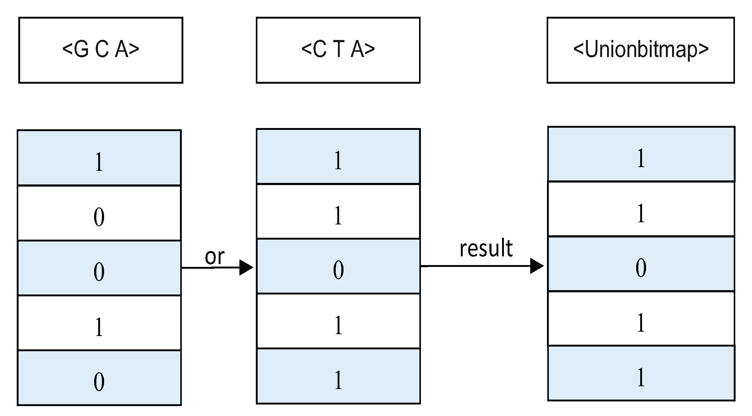
4.3. Calculating the Supports of Negative Sequences in f-NSP

We have adopted a new bitmap storage structure, where we can use the bit $OR$ operation to replace the original union operation. Assuming that s is a positive sequence, its bitmap is represented by $B\left(s\right)$, and the number ${}^{\prime }{1}^{\prime }$ in the bitmap is represented by N(B(s)). Subsequently, a negative sequence $ns$ of m-$size$ and n-$neg$-$size$ is given, and its support degree is:

$$sup\left(ns\right)=sup\left(MPS\left(ns\right)\right)-N\left(O{R}_{i=1}^n\left\{B\left(p\left(1-negM{S}_i\right)\right)\right\}\right)$$

(1)

Figure 1 explains the bit OR operation. If a positive sequence is <G C T A>, then $sup\left(CA\right)$ = 5. According to the negative candidate generation method, a negative candidate sequence $ns$ is <¬G C ¬T A>. The corresponding MPS($ns$) = <C A>, $P(1$-$negM{S}_1)$ = <G C A>, and $P(1$-$negM{S}_2)=$ <C T A>. Assuming that B(<$GCA$>) = |1|0|0|1|0|, B(<$CTA$>) = |1|1|0|1|1|. Subsequently, Figure 1 shows the bitmap union bitmap of B(<$GCA$>) OR B(<$CTA$>). Therefore, we can easily obtain N(unionbitmap) = 4, and then obtain $sup(<$¬G C ¬T A$>)$ = 1 from Equation (1).

If $ns$ only contains one negative element, then the support of sequence $ns$ is obtained by the Equation (2).

$$sup\left(ns\right)=sup\left(MPS\left(ns\right)\right)-sup\left(p\left(ns\right)\right)$$

(2)

In particular, the support for a single element negative sequence <¬G> is obtained by the Equation (3).

$$sup\left(〈\neg G〉\right)=\left|D\right|-sup\left(〈G〉\right)$$

(3)

4.4. The f-NSP Algorithm

Algorithm 1 shows the f-NSP algorithm. The information of the algorithm can be found in Dong [7].

Algorithm 1:f-NSP Algorithm.

1: Input: Sequence dataset (D) and minimum support(min_sup); 2: Output: NSP; 3: PSP=GSP(D); 4: HashTable PSPHash=CreatPSPHashTable(PSP); 5: for each psp in PSP do 6:     NSC=NSC_Generation(psp); 7:     for each nsc in NSC do 8:         if (nsc.size==1 &&nsc.nsize==1) then 9:            nsc.support=|D|-p(nsc).support; 10:         end if 11:         if (nsc.size>1 && nsc.nsize==1) then 12:            nsc.support=MPS(nsc).support-P(nsc).support; 13:         else 14:            1-$negMS{S}_{nsc}$={1-$negM{S}_i$|1<=i<=nsc.nsize}; 15:            Bitmap unionbitmap=1-$negM{S}_1$.getBitmap; 16:            for i = 2; i<=1-$negMS{S}_{nsc}$.size; i++ do 17:                unionbitmap=OR(1-$negM{S}_i$.getBitmap); 18:            end for 19:            nsc.support=MPS(nsc).support-unionbitmap.GetOneSize(); 20:         end if 21:         if (nsc.support_count/|D|>=min_sup) then 22:            NSP.add(nsc); 23:         end if 24:     end for 25: end for 26: Return NSP.

5. Similarity Analysis of Negative DNA Sequences

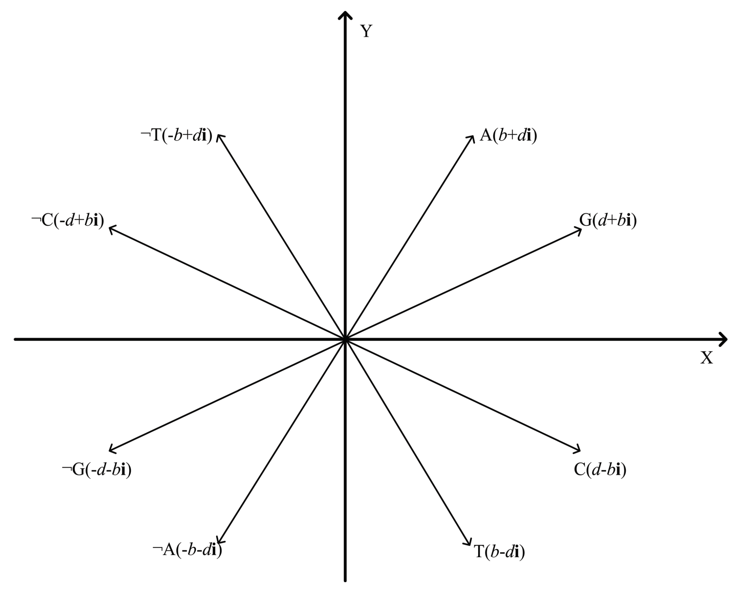
5.1. 2-D Representation of Negative DNA Sequential Patterns

Bai et al. [33] proposed a similarity analysis method for the positive sequential sequence. Based on this, we first propose a similarity analysis method for negative sequential patterns. We constructed a purine-pyrimidine diagram on the complex plane, as shown in Figure 2. The first and third quadrants are purines (A, ¬A, G and ¬G), the second and fourth quadrants are pyrimidines (T, ¬T, C and ¬C), which represent the unit vectors of the eight nucleotides A, ¬A, G, ¬G, C, ¬C, T and ¬T, and their corresponding sequences are as follows:

$$\left(b+di\right)\to \mathrm{A}, \left(d+bi\right)\to \mathrm{G}$$

$$\left(b-di\right)\to \mathrm{T}, \left(d-bi\right)\to \mathrm{C}$$

$$\left(-b-di\right)\to \neg \mathrm{A}, \left(-d-bi\right)\to \neg \mathrm{G}$$

$$\left(-b+di\right)\to \neg \mathrm{T}, \left(-d+bi\right)\to \neg \mathrm{C}$$

where b and d are non-zero real numbers. Here, we have $b=1\setminus 2$, $d=\sqrt{3}\setminus 2$. A and T are conjugate, ¬A and ¬T are conjugate, C and G are conjugate, ¬C and ¬G are conjugate. A, T, C, G stands for the existing base pair. Additionally, ¬A, ¬T, ¬C, ¬G stands for the base pair that should have appeared but did not (or the missing base pair), and is termed the negative base, as shown in Figure 2.

By this means, we can restore each frequent sequence pattern to a set of vectors. We numbered the DNA sequence and then thought of it as a finite complete ordered set with t elements, which is the same as $\left[t\right]=\left\{1,2,...,t\right\}$.

$$s\left(n\right)=s\left(0\right)+\sum _{j=1}^{n}y\left(j\right),n\in \left[t\right]$$

(4)

where $s\left(0\right)=0$, and $y\left(j\right)$ satisfies the following situation (see Equation (5)).

$$y\left(j\right)=\left\{\begin{array}{cc}\hfill & \frac{1}{2}+\frac{\sqrt{3}}{2}i,\mathrm{if}j=A,\hfill \\ \hfill & \frac{\sqrt{3}}{2}+\frac{1}{2}i,\mathrm{if}j=G,\hfill \\ \hfill & \frac{1}{2}-\frac{\sqrt{3}}{2}i,\mathrm{if}j=T,\hfill \\ \hfill & \frac{\sqrt{3}}{2}-\frac{1}{2}i,\mathrm{if}j=C,\hfill \\ \hfill & -\frac{1}{2}-\frac{\sqrt{3}}{2}i,\mathrm{if}j=\neg A,\hfill \\ \hfill & -\frac{\sqrt{3}}{2}-\frac{1}{2}i,\mathrm{if}j=\neg G,\hfill \\ \hfill & -\frac{1}{2}+\frac{\sqrt{3}}{2}i,\mathrm{if}j=\neg T,\hfill \\ \hfill & -\frac{\sqrt{3}}{2}+\frac{1}{2}i,\mathrm{if}j=\neg C,\hfill \end{array}\right.$$

(5)

$j=0,1,2,...,n$, where j represents the base type at the 0, 1, 2,..., n-th position in the sequence S, and n is the length of the DNA sequence being studied. We can uniquely obtain the original DNA sequence in the DNA diagram by connecting the points on the curve.

5.2. Algorithm Principle of DTW Distance

Set the time series $S^1\left(t\right)=\left\{s_1^1,s_2^1,...,s_m^1\right\}$, $S^2\left(t\right)=\left\{s_1^2,s_2^2,...,s_n^2\right\}$, and the lengths are m and n, respectively. According to their position time sorting, construct the matrix $A_{m\times n}$ of $m\times n$, and each element of the matrix, $a_{ij}=d\left(s_i^1,s_j^2\right)=\sqrt{{\left(s_i^1-s_j^2\right)}^2}$. In the matrix, the collection of a group of adjacent matrix elements is called the winding path, which is denoted as $W=w_1,w_2,...,w_k$, the k-$th$ element of W is $w_k={\left(a_{ij}\right)}_k$ and this path is used in order to satisfy the following conditions: (1) $max\left\{m,n\right\}\le K\le m+m-1$; (2) $w_1=a_{11}$, $w_k=a_{mn}$; and, (3) for $w_k=a_{ij}$, $w_{k-1}=a_{i^{{}^{\prime }}{j}^{{}^{\prime }}}$ must meet $0\le i-i^{{}^{\prime }}\le 1$, $0\le j-j^{{}^{\prime }}\le 1$, then $DTW\left(S^1,S^2\right)=min\left(\frac{1}{k}\sqrt{{\sum }_{i=1}^k{w}_i}\right)$. The DTW algorithm can be summarized in order to apply the idea of dynamic programming to find an optimal path to the smallest bending cost, namely,

$$\left\{\begin{array}{c}D\left(1,1\right)=a_{11}\hfill \\ D\left(i,j\right)=a_{ij}+min\left\{D\left(i-1,j-1\right),D\left(i,j-1\right),D\left(i-1,j\right)\right\}\hfill \end{array}\right.$$

(6)

Of these, $i=2,3,...,m.$$j=2,3,...,n.$ $D(m,n)$ is the minimum cumulative value of the bending path in $A_{m\times n}$.

5.3. Similarity Analysis of Negative DNA Sequences

Because the DNA sequence corresponds to its time series of one-to-one [33], the similarity of DNA sequences can only be compared by comparing the similarity of their corresponding time series. The DTW algorithm is one of the classical methods used to measure the similarity of the time series. The DTW distance algorithm is used here in order to compare the similarity of DNA sequences.

6. Experiment Results

We first used the f-NSP algorithm to obtain frequent sequence patterns, and then used the mined maximum frequent sequence patterns for similarity analysis. All of the experiments were performed on an Intel Core i5 computer with a 2.4-GHz CPU and 8 GB of memory, as well as using the Windows 7 operating system.

6.1. Experiment Data Set

Because the DNA sequence corresponds to its time series one to one, the similarity of the DNA sequence can only be compared by comparing the similarity of their corresponding time series. We compared the results of the frequent patterns mining of the first exon of the $\beta$-protein gene of the 10 different species based on our proposed graphical representation.

Table 2. The coding sequences of the first exon of the $\beta$-globin gene of 10 different species.

Data Set	Code Sequences
Human	ATGGTGCACCTGACTCCTGAGGAGAAGTCTGCCGTTACTGCCCTGTGGGGCAAGGTGAACGTGGATTAAGTTGGTGGTGAGGCCCTGGGCAG
Opossum	ATGGTGCACTTGACTTCTGAGGAGAAGAACTGCATCACTACCATCTGGTCTAAGGTGCAGGTTGACCAGACTGGTGGTGAGGCCCTTGGCAG
Rat	ATGGTGCACCTAACTGATGCTGAGAAGGCTACTGTTAGTGGCCTGTGGGGAAAGGTGAACCCTGATAATGTTGGCGCTGAGGCCCTGGGCAG
Chimpanzee	ATGGTGCACCTGACTCCTGAGGAGAAGTCTGCCGTTACTGCCCTGTGGGGCAAGGTGAACGTGGATGAAGTTGGTGGTGAGGCCCTGGGCAGGTTGGTATCAAGG
Gallus	ATGGTGCACTGGACTGCTGAGGAGAAGCAGCTCATCACCGGCCTCTGGGGCAAGGTCAATGTGGCCGAATGTGGGGCCGAAGCCCTGGCCAG
Goat	ATGCTGACTGCTGAGGAGAAGGCTGCCGTCACCGGCTTCTGGGGCAAGGTGAAAGTGGATGAAGTTGGTGCTGAGGCCCTGGGCAG
Gorilla	ATGGTGCACCTGACTCCTGAGGAGAAGTCTGCCGTTACTGCCCTGTGGGGCAAGGTGAACGTGGATGAAGTTGGTGGTGAGGCCCTGGGCAGG
Lemur	ATGACTTTGCTGAGTGCTGAGGAGAATGCTCATGTCACCTCTCTGTGGGGCAAGGTGGATGTAGAGAAAGTTGGTGGCGAGGCCTTGGGCAG
Mouse	ATGGTGCACCTGACTGATGCTGAGAAGTCTGCTGTCTCTTGCCTGTGGGCAAAGGTGAACCCCGATGAAGTTGGTGGTGAGGCCCTGGGCAGG
Rabbit	ATGGTGCATCTGTCCAGTGAGGAGAAGTCTGCGGTCACTGCCCTGTGGGGCAAGGTGAATGTGGAAGAAGTTGGTGGTGAGGCCCTGGGC

shows the coding sequences of the first exon of the $\beta$-globin gene of the 10 different species. Additionally,

Table 3. Information of the first exon of the $\beta$-globin gene of the 10 different species.

No.	Species	GenBank Accession Number	Location	Nucleotide Length
1	Human	U01317	62,187–62,278	92
2	Opossum	J03643	467–558	92
3	Rat	X06701	310–401	92
4	Chimpanzee	X02345	4189–4293	104
5	Gallus	V00409	465–556	92
6	Goat	M15387	279–364	86
7	Gorilla	X61109	4538–4630	93
8	Lemur	M15734	154–245	92
9	Mouse	V00722	259–367	93
10	Rabbit	V00882	277–366	90

lists the sequences information.

6.2. Result of Mining Patterns

Two positive and one negative maximum frequent sequential patterns of the 10 species were selected as the data set, as shown in

Table 4. 30 frequent sequential patterns.

Data Set	Frequent Pattern	Data Set	Frequent Pattern
Human1 (Hum1)	G T G G A G	Goat (Goa1)	G G T G G T
Human2 (Hum2)	G G G G G A	Goat (Goa2)	G C C T G C
Human3 (Hum3)	¬A G T G ¬C G A ¬C G	Goat (Goa3)	C ¬A T G A ¬A G ¬A
Opossum1 (Opo1)	G G C G C A	Gorilla (Gor1)	G G G G C A
Opossum2 (Opo2)	G G C T T A	Gorilla (Gor2)	G T G G A G
Opossum3 (Opo3)	G G C ¬G G C A ¬G	Gorilla (Gor3)	¬A G G G ¬C G A G
Rat1	G C C T G A	Lemur (Lem1)	G G G G G C
Rat2	G G T G G G	Lemur (Lem2)	G T G G C A
Rat3	G C C ¬A T G A ¬C	Lemur (Lem3)	¬A G T G ¬C G ¬T C A
Chimpanzee1 (Chi1)	G G G G A G	Mouse (Mou1)	T G G G G G
Chimpanzee2 (Chi2)	G T G G A G	Mouse (Mou2)	G G C C T G
Chimpanzee3 (Chi3)	¬A G G G ¬C G A G	Mouse (Mou3)	G C C ¬A T G ¬A C
Gallus (Gal1)	G G C G C T	Rabbit (Rab1)	G G T G G C
Gallus (Gal2)	G G C T T C	Rabbit (Rab2)	C C T G A T
Gallus (Gal3)	G G C ¬G G G	Rabbit (Rab3)	¬A T G A ¬C T G

. The min_sup was set to 0.3 during mining.

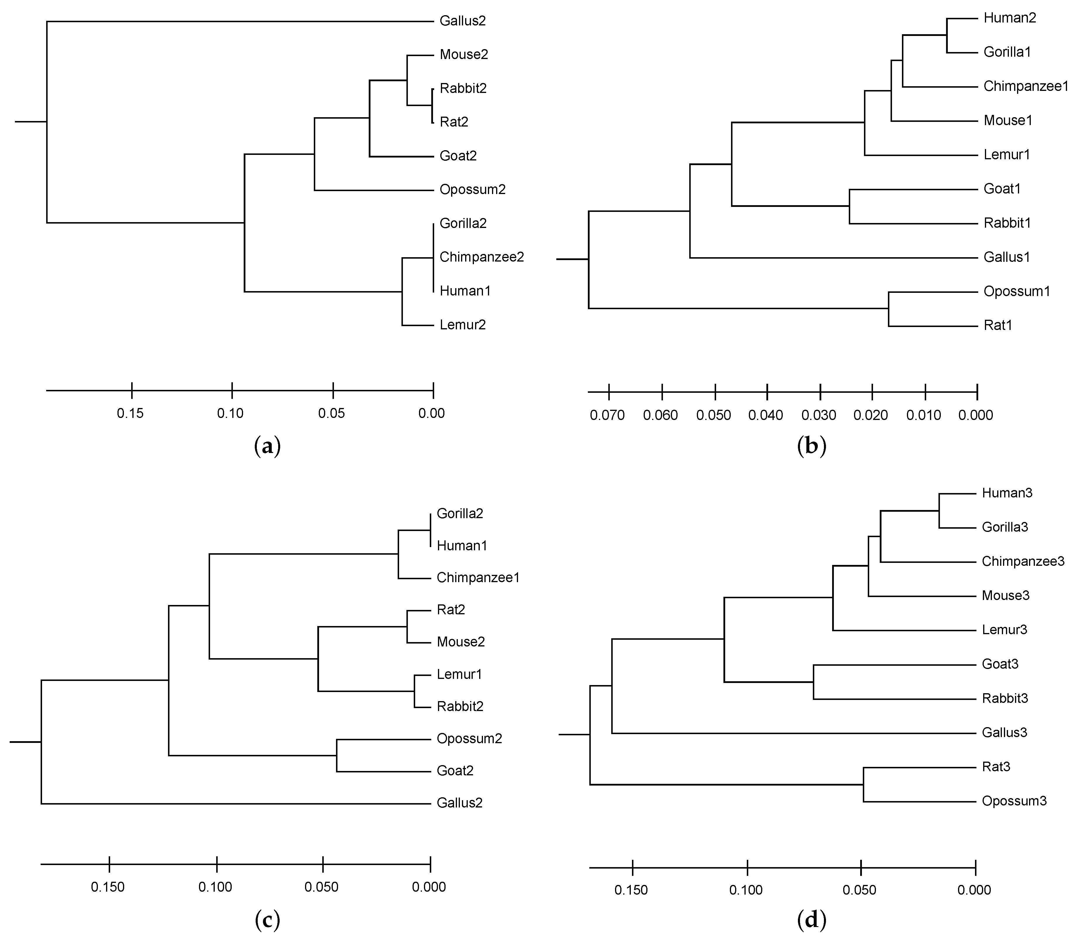
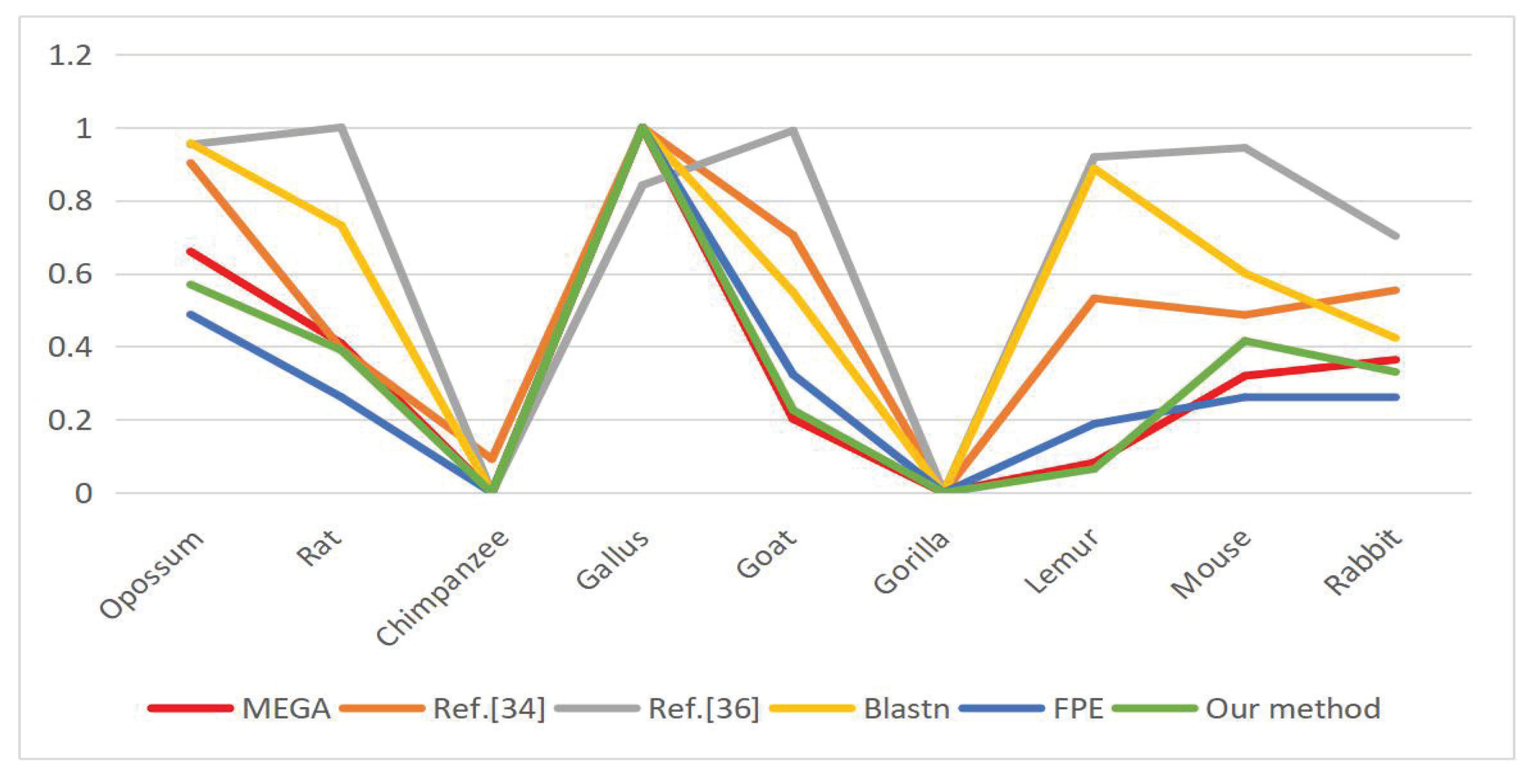
6.3. DNA Sequence Similarity Analysis

First, we used Equations (4) and (5) to convert 30 sequential patterns into the time series. Subsequently, we utilized the DTW distance algorithm in order to calculate the distance between two sequences. Finally, we obtained the distance matrix between the frequent patterns of the 10 species, as shown in

Table 5. Distance matrices between 20 frequent PSPs.

Frequent PSPs	Hum1	Hum2	Opo1	Opo2	Rat1	Rat2	Chi1	Chi2	Gal1	Gal2	Goa1	Goa2	Gor1	Gor2	Lem1	Lem2	Mou1	Mou2	Rab1	Rab2
Hum1	0.0000	X	0.1451	0.2739	0.1319	0.1876	0.0310	0.0000	0.1021	0.4808	0.0902	0.1086	0.0115	0.0000	0.1288	0.0313	0.0462	0.1998	0.0731	0.1589
Hum2		0.0000	0.1390	0.8654	0.1355	0.3845	0.0297	0.0992	0.0978	0.9575	0.0864	0.6786	0.0115	0.0121	0.0311	0.5149	0.0299	0.4719	0.0701	0.5361
Opo1			0.0000	X.XXXX	0.0339	0.0354	0.1510	0.1201	0.1690	0.0720	0.1594	0.0829	0.1497	0.1393	0.1560	0.1298	0.1535	0.1289	0.1675	0.1018
Opo2				0.0000	0.5405	0.1163	0.2513	0.2739	0.7460	0.2069	0.5194	0.1653	0.8670	0.2739	0.2411	0.3052	0.4471	0.0741	0.3881	0.1150
Rat1					0.0000	X	0.1374	0.1274	0.1527	0.0446	0.1399	0.1074	0.1360	0.1295	0.1387	0.1147	0.1385	0.1419	0.1429	0.0970
Rat2						0.0000	0.2081	0.1576	0.8291	0.3232	0.5142	0.0503	0.3871	0.1576	0.1557	0.1889	0.2025	0.0422	0.3168	0.0013
Chi1							0.0000	X	0.1090	0.1137	0.0774	0.0808	0.0276	0.0288	0.0443	0.0462	0.0411	0.0523	0.0764	0.0798
Chi2								0.0000	0.9591	0.4808	0.7322	0.1086	0.0937	0.0000	0.5479	0.0313	0.5200	0.1998	0.5720	0.1589
Gal1									0.0000	X	0.1388	0.1449	0.0979	0.1021	0.0829	0.0865	0.1296	0.1353	0.1083	0.1130
Gal2										0.0000	1.0320	0.3722	0.9600	0.4808	0.3009	0.5121	0.8288	0.2810	0.6227	0.3219
Goa1											0.0000	X	0.0873	0.0911	0.1052	0.1098	0.1332	0.0480	0.0488	0.0509
Goa2												0.0000	0.0641	0.1086	0.2352	0.1399	0.3309	0.0912	0.4349	0.0503
Gor1													0.0000	X	0.0274	0.0286	0.0278	0.0498	0.0732	0.0764
Gor2														0.0000	0.2123	0.0313	0.4702	0.1998	0.5354	0.1589
Lem1															0.0000	X	0.0696	0.0727	0.0913	0.0953
Lem2																0.0000	0.3877	0.2311	0.2671	0.1902
Mou1																	0.0000	X	0.1342	0.0461
Mou2																		0.0000	0.1572	0.0096
Rab1																			0.0000	X
Rab2																				0

and

Table 6. Distance matrices between 10 frequent negative sequential patterns (NSPs).

Frequent PSPs	Hum3	Opo3	Rat3	Chi3	Gal3	Goa3	Gor3	Lem3	Mou3	Rab3
Hum3	0.0000	0.4038	0.3671	0.0862	0.2843	0.2511	0.0321	0.0902	0.0886	0.2035
Opo3		0.0000	0.0985	0.3341	0.3403	0.2307	0.3878	0.3613	0.3587	0.2832
Rat3			0.0000	0.3544	0.3240	0.2989	0.3602	0.3191	0.3950	0.2700
Chi3				0.0000	0.3165	0.2248	0.0803	0.1286	0.1156	0.2220
Gal3					0.0000	0.4034	0.2841	0.2408	0.3766	0.3145
Goa3						0.0000	0.2537	0.3055	0.1336	0.1417
Gor3							0.0000	0.0795	0.0787	0.2127
Lem3								0.0000	0.2023	0.2653
Mou3									0.0000	0.1283
Rab3										0.0000

.

Here, we introduce the similarity analysis process of the sequences in detail. For example, the complex number sequence that is obtained by the sequence Human1 through Equations (4) and (5) is s(H1) = {0.866 + 0.5i, 1.366 − 0.366i, 2.2321 + 0.134i, 3.0981 + 0.634i, 3.5981 + 1.5i, and 4.4641 + 2i}. The time series made up of modules is S(H1) = {1.0000, 1.4142, 2.2361, 3.1623, 3.8982, and 4.8916}. Similarly, we obtained the time series after the transformation of the other 29 frequent sequences and we used our method to calculate the similarity with different data groups listed in Table 4, and the results are given in Table 5 and Table 6.

The phylogenetic tree was generated according to the distance matrix. A phylogenetic tree is a tree-like branching graph that summarizes the genetic or evolutionary relationships of various organisms. Here, we used MEGA-X to construct our phylogenetic tree. If it could be reasonably constructed, as shown in Figure 3, different sequence combinations would provide different results, but all of them were consistent with the evolutionary genetic relationship among organisms. For example, we noted that the results of the phylogenetic tree of Hum1, Opo2, Rat2, Chi2, Gal2, Goa2, Gor2, Lem2, Mou2, and Rab2 were the same as those in citation [34], and this introduced a group representation vector to represent each protein sequence to generate a similar/different vector, rather than a regular similar/different matrix. The phylogenetic tree of Hum2, Opo1, Rat1, Chi1, Gal1, Goa1, Gor1, Lem1, Mou1, and Rab1 were similar to [16]. The phylogenetic tree of Hum1, Opo2, Rat2, Chi1, Gal2, Goa2, Gor2, Lem1, Mou2, and Rab2 were the same as that in [35], which constructs a graphic representation of the DNA sequence according to the Fermat spiral curve. When considering the local characteristics of the DNA sequence, each point on the Fermat spiral curve then related to the corresponding mass according to the relationships between the four adjacent nucleotides. The homology of the selected NSP combination was similar to the result presented in [16], but there was still a certain gap between them in terms of evolutionary matrix. Because more than one maximum frequency pattern was mined, and this was particularly true of NSPs, we could derive more pattern combinations and, thus, more evolutionary relationships between species, particularly those that were missing some of their bases, which we could still effectively partition.

We compared the first group of frequent pattern combinations that were obtained above with three existing methods and Blastn [36]. By using Blasten, we will obtain a score, and our results can be directly generated by using the software. Readers can refer to https://blast.ncbi.nlm.nih.gov/. The higher the score, the better the homology and the closer the distance. For the other three methods, the one proposed by Mo et al. [35] in 2018, and the other by Yu [37]. The third method is FPE, as proposed by Xie et al. [31], which used the prefix span algorithm to find the maximum frequency pattern, and then calculated the entropy of each block according to the probability of the pattern, and finally constitutes the vector component of the sequence by the obtained entropy. MEGA is a well-known alignment based tool, called Sequence Alignment Tools, so, here, we also used the results of MEGA [38] software as a benchmark. Molecular Evolutionary Genetics Analysis version 5 (MEGA5), user friendly software for online mining databases, was used to build sequence alignments and phylogenetic trees. It is available free of charge from http://www.megasoftware.net. MEGA software development is currently supported by research grants from the National Institutes of Health. The Pearson correlation coefficients between the results of our method and the four comparison methods and the results of MEGA were calculated.

Table 7. Comparison of the distances between humans and the other species.

	Opo- Ssum	Rat	Chimp- Anzee	Gallus	Goat	Gorilla	Lemur	Mouse	Rabbit	CORREL
MEGA	0.4823 (0.6600)	0.2985 (0.0000)	0.0000 (0.0000)	0.7308 (1.0000)	0.1599 (0.2188)	0.0000 (0.0000)	0.0600 (0.0821)	0.2336 (0.3197)	0.2659 (0.3639)	X
Z.Y.Mo. [35]	0.2696 (0.9026)	0.1198 (0.3939)	0.0309 (0.0920)	0.2983 (1.0000)	0.2114 (0.7049)	0.0038 (0.0000)	0.1604 (0.5318)	0.1470 (0.4863)	0.1670 (0.5542)	0.8327
H.J.Yu. [36]	25.9952 (0.9531)	27.0102 (1.0000)	5.3704 (0.0000)	23.5869 (0.8418)	26.8209 (0.9913)	5.3704 (0.0000)	25.2515 (0.9187)	25.8007 (0.9441)	20.5706 (0.7024)	0.5294
Blastn	0.9567 (0.9567)	0.7315 (0.7315)	0.0000 (0.0000)	1.0000 (1.0000)	0.5486 (0.5486)	0.0000 (0.0000)	0.8874 (0.8874)	0.6008 (0.6008)	0.4235 (0.4235)	0.7323
FPE	0.1237 (0.4876)	0.0664 (0.2617)	0.0000 (0.0000)	0.2537 (1.0000)	0.0820 (0.3232)	0.0000 (0.0000)	0.0478 (0.1884)	0.0663 (0.2613)	0.0664 (0.2617)	0.9505
Our method	0.2739 (0.5697)	0.1876 (0.3902)	0.0000 (0.0000)	0.4808 (1.0000)	0.1086 (0.2259)	0.0000 (0.0000)	0.0313 (0.0651)	0.1998 (0.4156)	0.1589 (0.3305)	0.9887

outlines the distance between the six methods and the other species and humans. The values in the brackets are the true distances that are normalized to a range between 0 and 1. We processed the score data of BLASTn according to the method that was proposed by Xie [31]. Finally, the Pearson correlation coefficient between the results of our method and the four comparison methods was calculated. Our method had the highest correlation coefficient with MEGA and, thus, our method had the highest correlation with MEGA, indicating that our method could more accurately calculate the similarity between DNA sequences. In addition, Figure 4 shows that the curve of our method was closer to that calculated while using the MEGA method, which again indicates that our method had the highest correlation with it.

We learned that the overall variation of our method was consistent with the other comparison methods, so the method that was proposed in this paper was effective and feasible. We experimentally proved that our method was more accurate than other methods and that the proposed method is applicable for both short and long sequences. Because the data we used were frequent patterns after mining, the length of the sequence used for comparison was generally shortened and the characteristics of the original sequence were retained. The calculation was simple and memory consumption of the computer was reduced. In addition, more than one maximum frequency pattern was mined and this was particularly true of NSPs. Therefore, more pattern combinations could be derived. By comparing the similarities among the 10 species, we saw that various combinations of patterns yielded unique results, which may be useful for various considerations.

7. Conclusions Future Work

We proposed a DNA sequence representation and similarity analysis method based on frequent patterns, which were presented as eight vectors in a 2-D space. The frequent pattern consisted of the frequent pattern in general and the frequent pattern with some bases missing. Different pattern combinations have unique evolutionary results, which can adequately classify species. Some noise could be tolerated because we only considered maximum frequency patterns and retained the characteristics of the sequence. Our method reduced the consumption of computer memory by a large amount. The calculations were very simple. Testing the $\beta$-globin gene of 10 species showed that our method shared similarities to several recently developed alignment-free methods. Crucially, the correlation comparison of several methods and MEGA showed that our results had the highest correlation, indicating that our method more accurately calculated the similarity between DNA sequences.

Our future work will be to find a more effective way to mine biological sequences, which will not only maintain the continuity of biological sequences, but also effectively mine NSPs. In addition, we aim to find a method for selecting optimal frequent patterns in order to reduce the errors in similarity analysis.

References

1. Zhang, W.; Wang, X.; Huang, Z. A System of Mining Semantic Trajectory Patterns from GPS Data of Real Users. Sysmmetry 2019, 11, 889. [Google Scholar] [CrossRef] [Green Version]
2. Zhang, J.; Wang, Y.; Zhang, C.; Shi, Y. Mining Contiguous Sequential Generators in Biological Sequences. IEEE/ACM Trans. Comput. Biol. Bioinform. 2016, 13, 855–867. [Google Scholar] [CrossRef] [PubMed]
3. Matloob, I.; Khan, S.; Rehman, H. Sequence Mining and Prediction-Based Healthcare Fraud Detection Methodology. IEEE Access 2020, 8, 143256–143273. [Google Scholar] [CrossRef]
4. Cao, L.; Yu, P.; Kumar, V. Nonoccurring Behavior Analytics: A New Area. IEEE Intell. Syst. 2015, 30, 4–11. [Google Scholar] [CrossRef]
5. Jiang, X.; Xu, T.; Dong, X. Campus Data Analysis Based on Positive and Negative Sequential Patterns. Int. J. Pattern Recognit. Artif. Intell. 2019, 33. [Google Scholar] [CrossRef]
6. Cao, L.; Dong, X.; Zheng, Z. e-NSP: Efficient negative sequential pattern mining. Artif. Intell. 2016, 235, 156–182. [Google Scholar] [CrossRef] [Green Version]
7. Dong, X.; Gong, Y.; Cao, L. F-NSP+: A fast negative sequential patterns mining method with self-adaptive data storage. Pattern Recognit. 2018, 84, 13–27. [Google Scholar] [CrossRef]
8. Katoh, K.; Asimenos, G.; Toh, H. Multiple alignment of DNA sequences with MAFFT. Methods Mol. Biol. 2009, 537, 39–64. [Google Scholar]
9. Paterson, A.; Freeling, M.; Tang, H.; Wang, X. Insights from the Comparison of Plant Genome Sequences. Annu. Rev. Plant Biol. 2010, 61, 349–372. [Google Scholar] [CrossRef]
10. Eugene, H.; John, R. A novel method of representation of nucleotide series especially suited for long DNA sequences. J. Biol. Chem. 1983, 258, 1318–1327. [Google Scholar]
11. Liao, B.; Wang, T.; Huang, Z. New 2D graphical representation of DNA sequences. J. Comput. Chem. 2004, 25, 1364–1368. [Google Scholar] [CrossRef] [PubMed] [Green Version]
12. Gong, W.; Fan, X. A geometric characterization of DNA sequence. Phys. A Stat. Mech. Its Appl. 2019, 527, 121429. [Google Scholar] [CrossRef]
13. Guo, Y.; Wang, T.; Huang, Z. A new method to analyze the similarity of the DNA sequences. Comput. Theor. Chem. 2008, 853, 62–67. [Google Scholar] [CrossRef]
14. Ma, T.; Liu, Y.; Dai, Q.; Yao, Y.; He, P. A graphical representation of protein based on a novel iterated function system. Phys. A Stat. Mech. Its Appl. 2014, 403, 21–28. [Google Scholar] [CrossRef]
15. Lee, S.; Cha, J.; Theera-Umpon, N.; Kim, K. Analysis of a Similarity Measure for Non-Overlapped Data. Symmetry 2017, 9, 68. [Google Scholar] [CrossRef] [Green Version]
16. Xie, G.; Jin, X.; Yang, C.; Pu, J.; Mo, Z. Graphical Representation and Similarity Analysis of DNA Sequences Based on Trigonometric Functions. Acta Biotheor. 2018, 66, 113–133. [Google Scholar] [CrossRef]
17. Aboelkhier, M.; Abdelwahaab, M.; Aboelmaaty, M. Measuring Similarity among Protein Sequences Using a New Descriptor. BioMed Res. Int. 2019, 2019, 2796971. [Google Scholar]
18. Jafarzadeh, N.; Iranmanesh, A. C-curve: A novel 3D graphical representation of DNA sequence based on codons. Math. Biosci. 2013, 241, 217–224. [Google Scholar] [CrossRef]
19. Liao, B.; Xiang, Q.; Cai, L.; Cao, Z. A new graphical coding of DNA sequence and its similarity calculation. Phys. A Stat. Mech. Its Appl. 2013, 392, 4663–4667. [Google Scholar] [CrossRef]
20. Olivier, D.; Eric, R. STAR: An algorithm to Search for Tandem Approximate Repeats. Bioinformatics 2004, 20, 2812–2820. [Google Scholar]
21. Kurtz, S.; Choudhuri, J.; Ohlebusch, E.; Schleiermacher, C.; Stoye, J.; Giegerich, R. REPuter: The manifold applications of repeat analysis on a genomic scale. Nucleic Acids Res. 2001, 29, 4633–4642. [Google Scholar] [CrossRef] [PubMed] [Green Version]
22. Deng, N.; Chen, X.; Li, S.; Xiong, C. Frequent Patterns Mining in DNA Sequence. IEEE Access 2019, 7, 108400–108410. [Google Scholar] [CrossRef]
23. Zhang, J.; Guo, J.; Zhang, M.; Yu, X.; Yu, X.; Guo, W.; Zeng, T.; Chen, L. Efficient Mining Multi-mers in a Variety of Biological Sequences. IEEE/ACM Trans. Comput. Biol. Bioinform. 2018, 17, 949–958. [Google Scholar] [CrossRef] [PubMed]
24. Hsueh, J.; Lin, M.; Chen, C. Mining Negative Sequential Patterns for E-commerce Recommendations. In Proceedings of the 3rd IEEE Asia-Pacific Service Computing Conference, Yilan, Taiwan, 9–12 December 2008; pp. 1213–1218. [Google Scholar]
25. Zheng, Z.; Zhao, Y.; Zuo, Y.; Cao, L. Negative-GSP: An efficient method for mining negative sequential patterns. In Proceedings of the 8th Australasian Data Mining Conference, Melbourne, Australia, 1–4 December 2009; pp. 63–67. [Google Scholar]
26. Rastogi, V.; Khare, V. Apriori Based: Mining Positive and Negative Frequent Sequential Patterns. Int. J. Latest Trends Eng. Technol. 2012, 1, 24–33. [Google Scholar]
27. Khare, V.; Rastogi, V. Mining Positive and Negative Sequential Pattern in Incremental Transaction Databases. Int. J. Comput. Appl. 2013, 71, 18–22. [Google Scholar]
28. Lin, N.; Chen, H.; Hao, H.; Wei, H. Mining negative sequential patterns. In Proceedings of the 6th WSEAS International Conference on Applied Computer Science, Corfu, Greece, 16–19 February 2007; pp. 654–658. [Google Scholar]
29. Dong, X.; Gong, Y.; Cao, L. e-RNSP: An Efficient Method for Mining Repetition Negative Sequential Patterns. IEEE Trans. Cybern. 2020, 50, 2084–2096. [Google Scholar] [CrossRef]
30. Dong, X.; Qiu, P.; Lu, J.; Cao, L.; Xu, T. Mining Top-k Useful Negative Sequential Patterns via Learning. IEEE Trans. Neural Netw. Learn. Syst. 2019, 30, 2764–2778. [Google Scholar] [CrossRef]
31. Xie, X.; Guan, J.; Zhou, S. Similarity evaluation of DNA sequences based on frequent patterns and entropy. BMC Genom. 2015, 16, S5. [Google Scholar] [CrossRef] [Green Version]
32. Jin, X.; Jiang, Q.; Chen, Y.; Lee, S.; Nie, R.; Yao, S.; Zhou, D.; He, K. Similarity/dissimilarity calculation methods of DNA sequences: A survey. J. Mol. Graph. Model. 2017, 76, 342–355. [Google Scholar] [CrossRef]
33. Bai, F.; Wang, T. A 2-D graphical representation of protein sequences based on nucleotide triplet codons. Chem. Phys. Lett. 2005, 413, 458–462. [Google Scholar] [CrossRef]
34. Abd Elwahaab, M.A.; Abo-Elkhier, M.M.; Abo el Maaty, M.I. A Statistical Similarity/Dissimilarity Analysis of Protein Sequences Based on a Novel Group Representative Vector. BioMed Res. Int. 2019, 2019, 1–9. [Google Scholar] [CrossRef] [PubMed] [Green Version]
35. Mo, Z.; Zhu, W.; Sun, Y.; Xiang, Q.; Zheng, M.; Chen, M.; Li, Z. One novel representation of DNA sequence based on the global and local position information. Sci. Rep. 2018, 8, 217–224. [Google Scholar] [CrossRef] [PubMed]
36. Altschul, S.; Madden, T.; Schäffer, A.; Zhang, J.; Zhang, Z.; Miller, W.; Lipman, D.J. Gapped BLAST and PSI-BLAST: A new generation of protein database search programs. Nucleic Acids Res. 1997, 25, 3389–3402. [Google Scholar] [CrossRef] [PubMed] [Green Version]
37. Yu, H.; Huang, D. Graphical representation for DNA sequences via joint diagonalization of matrix pencil. IEEE J. Biomed. Health Inform. 2013, 17, 503–511. [Google Scholar] [CrossRef]
38. Tamura, K.; Peterson, D.; Peterson, N.; Stecher, G.; Nei, M.; Kumar, S. Mega5: Molecular evolutionary genetics analysis using maximum likelihood, evolutionary distance, and maximum parsimony methodsn. Mol. Biol. Evol. 2011, 28, 2731–2739. [Google Scholar] [CrossRef] [Green Version]
Figure 1. Operation process of bit OR.
Symmetry 12 02090 g001
Figure 2. A purine–pyrimidine graph.
Symmetry 12 02090 g002
Figure 3. The phylogenetic tree was generated according to the distance matrix. (a) Hum1, Opo2, Rat2, Chi2, Gal2, Goa2, Gor2, Lem2, Mou2, and Rab2. (b) Hum2, Opo1, Rat1, Chi1, Gal1, Goa1, Gor1, Lem1, Mou1, and Rab1 (c) Hum1, Opo2, Rat2, Chi1, Gal2, Goa2, Gor2, Lem1, Mou2, and Rab2 (d) Negative sequential pattern combination.
Symmetry 12 02090 g003
Figure 4. Normalized species distance graph (the ordinate is the normalized distance).
Symmetry 12 02090 g004