A New Ensemble Learning Algorithm Combined with Causal Analysis for Bayesian Network Structural Learning

1
College of Meteorology and Oceanography, National University of Defense Technology, Nanjing 211101, China
2
Collaborative Innovation Center on Meteorological Disaster Forecast, Warning and Assessment, Nanjing University of Information Science and Engineering, Nanjing 210044, China
*
Author to whom correspondence should be addressed.
Symmetry 2020, 12(12), 2054; https://doi.org/10.3390/sym12122054
Submission received: 16 November 2020
/
Revised: 5 December 2020
/
Accepted: 7 December 2020
/
Published: 11 December 2020
(This article belongs to the Section Mathematics)
Abstract
:The Bayesian Network (BN) has been widely applied to causal reasoning in artificial intelligence, and the Search-Score (SS) method has become a mainstream approach to mine causal relationships for establishing BN structure. Aiming at the problems of local optimum and low generalization in existing SS algorithms, we introduce the Ensemble Learning (EL) and causal analysis to propose a new BN structural learning algorithm named C-EL. Combined with the Bagging method and causal Information Flow theory, the EL mechanism for BN structural learning is established. Base learners of EL are trained by using various SS algorithms. Then, a new causality-based weighted ensemble way is proposed to achieve the fusion of different BN structures. To verify the validity and feasibility of C-EL, we compare it with six different SS algorithms. The experiment results show that C-EL has high accuracy and a strong generalization ability. More importantly, it is capable of learning more accurate structures under the small training sample condition.
1. Instruction
In the era of Big Data, in order to obtain the scientific evaluation and decision, mathematical modeling for knowledge expression and inference, such as data mining and analysis, plays a crucial role, especially for complex problems with uncertain information and causal relationships. The Bayesian Network (BN), on the basis of probability theory and graph theory, is a powerful model for uncertainty expression and causality reasoning [1] and gets lots of attention in the area of defense, medicine and finance. BN modeling includes structural learning and parameter learning. Structural learning, considered the foundation of BN, is to construct a directed network topology based on objective data and priori knowledge [2]. At present, one of the research hotspots of BN is how to learn network structures accurately and efficiently from large datasets.
There are mainly two types of structural learning approaches: the Conditional Independence Testing method (CIT) and Search-Score method (SS). The key to CIT is to choose appropriate measure functions for the dependency test among network nodes, so as to find variable groups having independence relationships. The typical testing algorithms are mostly based on Chi-Square test and conditional mutual information, such as the SGS algorithm, EP algorithm and TPDA algorithm [3]. The employment of CIT is intuitive and easily understandable. Unfortunately, with the increase in network nodes, the complexity of CIT increases exponentially, causing low efficiency and unreliable results. By contrast, SS is more efficient in dealing with large-scale networks. It treats the structural learning as an optimization problem [4], that is, one search algorithm is used to find the optimal network structure in a network space constructed by all nodes, and the process is guided by one scoring function. SS is simple, convenient and feasible so it has become the mainstream method of BN structural learning [5].
Seen from the principle of SS methods, the scoring function and search algorithm are the two most important parts. The scoring function is used to evaluate structures and the optimal structure is found by search algorithms. With different scoring functions and search algorithms proposed, scholars have designed varieties of SS algorithms: Cooper [6] proposed the well-known K2 algorithm based on the Hill-Climbing (HC) algorithm, which needs the node order as prior information. Lam [7] improved the K2 algorithm into the K3 algorithm by using the Minimum Description Length (MDL) as the scoring function. In the case of small training samples, the K3 algorithm can get more accurate results than the K2 algorithm. Then, Heckeman [8] put forward another new scoring function, Bayesian Dirichlet equivalent (BDe), to improve the K2 algorithm. There is no need to obtain the node order in advance in this SS algorithm, which expands its application field.
However, there is a general consensus that the searching space is too large to find the optimum. Those SS algorithms have low searching efficiency and are easily trapped into local optimization [9]. To solve this problem, heuristic search algorithms in the field of intelligent optimization are introduced to search for the optimal structure. The Genetic Algorithm (GA), Particle Swarm Optimization (PSO), Ant Colony Optimization (ACO) and Artificial Bee Colony (ABC) algorithm have been applied to BN structural learning and achieved satisfactory results because of their global searching ability [10,11,12]. However, it is still a great challenge to obtain the global optimal structure as the structural learning from objective data is a typical NP-hard problem [13].
To further enhance the accuracy and efficiency of SS algorithms, some other improvement have also been made by modifying the scoring function or combining it with the CIT method. Campos [14] designed a new scoring function based on a Mutual Information Test (MIT), and the accuracy of network structure is measured by the Kullback–Leibler distance between the structure and observed data. Bouchaala [15] put forward a new scoring function, Implicit Score (IS), which uses the hidden estimation and avoids calculating probability distribution of variables in advance. Fan [16] analyzed the characteristics of the K2 algorithm and MCMC algorithm, and combined the advantages of both sides to propose an improved structural learning algorithm. This algorithm can obtain a stable structure efficiently without prior knowledge. Based on the unconstrained optimization and GA, Wang [17] constructed a restricted GA-based model for BN structural learning, leading to a significant reduction in search space. Li [18,19] introduced causal Information Flow theory to carry out causal analysis of structures in advance and improve initial network structures in searching process, which significantly enhances searching efficiency and effectively avoids premature convergence.
To some extent, the above-developed algorithms improve search spaces and scoring functions, increasing the accuracy and efficiency of structural learning. However, the algorithm optimization is restricted as learning network structure from a large-scale dataset remains the famous NP-hard problem [20]. Although a better network structure may be found, it is still easy to fall into the local optimal solution. In addition, more and more search algorithms and scoring functions are proposed, generating all kinds of SS algorithms. When applied to networks with different sizes and types, SS algorithms perform differently. Thus, it is difficult to select a reasonable search algorithm and scoring function. More importantly, each SS algorithm has a weak generalization ability. The performance of an algorithm is not stable when it deals with different networks. (More detailed discussion about performances of different SS algorithms will be elaborated in Section 2.)
Ensemble Learning (EL), an effective method of improvement of model performance in Machine Learning (ML), believes that if models are approximately independent of each other, the performance of an integrating model is better than that of an individual model [21]. EL is able to improve the accuracy and generalization of learning systems so it has become a hot topic of ML, which has been applied to face recognition, medical diagnosis and weather forecasting successfully [22,23]. Considering the differences between various SS algorithms, we will try to establish a new EL-based SS algorithm to improve the accuracy and generalization of structural learning. As we all know, the EL mechanism includes the base learner and integration way. Base learners are usually easy to be trained, but the integration way is hard to design and has a significant impact on EL effects [24]. BN expresses causal relationships among variables quantitatively. The high complexity of BN structure makes traditional fusion methods no longer applicable. Aiming at the causality of BN, we will introduce the causal Information Flow (IF) theory [25], an emerging causal analysis theory, to propose an improved weighted fusion way that is fit for the structure aggregation.
On the basis of EL and causal IF, we put forward a new BN structural learning algorithm, namely C-EL. We establish the EL mechanism of BN structures by the means of Bagging method. Then causal IF is introduced to construct a new weighted integration rule and the weight is calculated from the causality of BN. Our proposed model can achieve the fusion of various algorithms. The experiment results show that C-EL has high accuracy and strong generalization ability. More importantly, it is capable of learning more accurate structures under the small training sample condition. The rest of the paper is organized as follows: Section 2 explains the theoretical formulations and Section 3 discusses the existing problems of SS algorithms by contrast experiments. Detailed elaboration of the C-EL algorithm is presented in Section 4. Application of the proposed algorithm in structural learning and results analysis are elaborated in Section 5. Section 6 concludes the presented studies.
2. Basic Theory
2.1. Bayesian Network
The Bayesian Network (BN), also known as the Bayesian reliability network, is not only a graphical expression of causal relationships among variables but also a probabilistic reasoning technique [1]. It can be represented by a binary :
- represents a directed acyclic graph. is a set of nodes representing variables in the problem domain. is a set of arcs, and a directed arc represents the causal dependency between two variables.
- is the network parameter, that is, the probability distribution of each node. expresses the degree of mutual influence among nodes and presents quantitative characteristics in the knowledge domain.
Assuming a set of variables , the mathematical basis of BN is the Bayes Theorem shown as Equation (1).
where is the prior probability, is the conditional probability and is the posterior probability. Based on , can be derived by the Bayes Theorem under the relevant conditions .
The joint probability distribution of all nodes in the BN can be derived from Equation (1) under the assumption of conditional independence [19].
where is the node, is the parent node of . Equation (2), the core of Bayesian inference, can achieve the calculation of probability distribution of a set of query variables based on the evidence of input variables.
BN modeling mainly includes structural learning and parameter learning. Structural learning is the basis and prerequisite of parameter learning, which mines causal relationships from data and expresses them in the form of a network. It can be described as a process where, based on an observed dataset of the node set , the network structure that best matches can be found through intelligent learning algorithms [26,27]. SS algorithms are widely used for structural learning and achieving satisfactory results. We will make a specific introduction to it in the next subsection.
2.2. Search-Score Based Method
The basic idea of the SS method is: firstly, the scoring function is defined to measure the matching degree between the structure and training data. Then, an initial network is constructed and the search algorithm is applied to search for structures until the scoring function converges. The process can be described by the mathematical expression:
where is the score of a network based on dataset . is a function used to find the top-scoring structure.
Scoring function and search algorithm are the two important components of SS methods, which directly determine the accuracy and efficiency of structural learning. The earliest scoring function is the Bayesian Information Criterion (BIC) proposed by Schwarz in 1978 [28]. Later, a variety of scoring functions were developed, such as the K2 criterion, MDL, BDe and MIT mentioned in Instruction, for BN structural learning. In addition to scoring functions, search algorithms also play a pivotal role in the SS method [29]. As structure searching is the famous NP-hard problem, many intelligent algorithms, such as GA, PSO, ACO and ABC algorithm, have been applied to searching optimization. Besides, some scholars have constructed hybrid search algorithms by combining CIT, such as the sparse candidate algorithm and max-min hill-climbing algorithm [30]. The searching space of these algorithms is reduced, and convergence speed is improved by an independent relationship test.
Thus, there are all kinds of SS algorithms based on different scoring functions and search algorithms. How does the performance of different algorithms differ? What is the difference in the learning results of different networks with the same algorithm? Is there an algorithm with a strong generalization ability? In the next section, quantitative analysis of SS algorithms will be carried out through simulation experiments on the issues above.
3. Analysis of Search-Score Based Methods
In this section, we select different scoring functions and search algorithms for BN structural learning to discuss the performance of various SS algorithms from the view of accuracy and generalization. On the basis of studying many documents [12,14,18], the three most classical scoring functions, whose mathematical expressions are shown below, and the two most widely used search algorithms (HC and GA) are adopted for experiments, forming a total of six different SS algorithms: “BIC+HC”, “BIC+GA”, “MDL+HC”, “MDL+GA”, “BDe+HC” and “BDe+GA”.
- BIC criteria:
- MDL criteria:
- BDe criteria:
In the structural learning experiments, three representative BNs in different scales are used for algorithm verification: the Asia network composed of 8 nodes and 8 arcs, the Child network composed of 20 nodes and 25 arcs, and the Alarm network composed of 37 nodes and 46 arcs. The three standard networks have been widely used in previous studies of BN structural learning. According to the structure and conditional probability distribution of each BN, data sampling is conducted by means of the Full_BNT toolbox [31], and 1500 training samples of each network are collected randomly. Table 1 shows the training datasets of Asia network.
Hamming distance () defined by Equation (7) is used to measure the quality of learning structures [32]. The smaller the , the more accurate the network structure learned. In order to reduce the randomness of search algorithms, the structural learning is usually conducted multiple times. By referring to previous studies [17,18], we carry out each experiment ten times, and the average results are given in Table 2 and Figure 1.
where represents the number of lost arcs in learning structures, represents the number of excrescent arcs, and represents the number of reverse arcs.
From Table 2 and Figure 1, we can find that: (1) For the same network structure, the accuracy obtained by different algorithms varies greatly. The difference of between the best algorithm and the worst algorithm is obvious (Asia: 3.2/10.4; Child: 5.8/14.7; Alarm: 17.6/68.2). (2) For the same SS algorithm, the accuracy of different networks also varies greatly, such as “BIC+GA” and “BDe+HC” marked in yellow. For example, “BIC+GA” has good performance in the structural learning of Child, while it performs badly for Asia, indicating that generalization capabilities of the above algorithms are weak. (3) For Asia, Child and Alarm, the best learning algorithms are “BDe+HC”, “MDL+GA” and “BDe+GA”, respectively. In other words, there exists no algorithm that can learn the optimal structure of all networks. In conclusion, different algorithms used for BN structural learning have different learning performances, and the performance of the same algorithm is not stable when it deals with different networks.
It is not a good idea to choose the appropriate scoring function and search algorithm because there are all kinds of algorithms. Considering the visible differences of performance between various SS algorithms, we combine the Ensemble Learning with causal Information Flow theory to propose a new learning algorithm for BN structure (C-EL), aiming at improving the accuracy and stability of structural learning. The theoretical scheme and technical flow of the C-EL algorithm will be elaborated in detail in the next section.
4. Causality-Based Ensemble Learning Algorithm for BN Structure
In this section, we first make a brief introduction of Ensemble Learning and analyze its suitability in BN structural learning. Then, we put forward a new weighted integration rule based on the causal Information Flow theory. Finally, we elaborate on the technique process of our proposed algorithm based on the above parts. The three parts are logically combined internally and we will explain them specifically.
4.1. Ensemble Learning
Ensemble Learning (EL) is a kind of Machine Learning (ML) pattern. It uses multiple algorithms to learn and integrates all learning results with a certain rule, in order to improve accuracy and generalization of the learning system. The individual algorithm is called the base learner, and the rule of algorithm fusion is called the integration mechanism [33].
Research shows that the performance of the integrated learner is significantly higher than that of a single learner. The availability of EL can be concluded to two aspects [34]: On the one hand, it has been proved that the training of neural network or decision tree is the NP-hard problem, so heuristic search algorithms are usually adopted to solve the problem. Unfortunately, the optimal model is difficult to obtained in this way, but multi-model integration can be closer to the optimal result in theory. On the other hand, hypothesis spaces of ML algorithms are artificial and the actual objective in application scenarios may not be in the assumption space. EL can enrich the assumption space and express the objective that cannot be obtained by an individual ML algorithm, further significantly improving the generalization ability of learning system. In other words, the above advantages of EL can make up for the existing deficiencies of low accuracy and stability in SS algorithms.
Bagging and Boosting are the most basic methods in EL [33]. BN structural learning, focusing on expressing causal relationships among variables, is different from the conventional ML and its time complexity is even higher. Therefore, we adopt the Bagging method with parallel computation ability to construct the EL mechanism of structures, which contributes to improving the learning efficiency. Bagging, the abbreviation of Bootstrap Aggregating proposed by Breiman [35], uses the Bootstrapping algorithm for EL. Bootstrapping is a sampling method with replacement and is used to generate different training datasets for each base learner. The Algorithm 1 flow of Bagging is presented as follows:
| Algorithm 1 EL with the Bagging method |
| Input: Original data ; Base leaner Output: Integrating model Step 1: Sampling Training sets are extracted from with Bootstrapping; A total of rounds are taken, and samples are extracted in each round. Step 2: Training Each time one training set is used to train a model, and training sets can generate models. Step 3: Integration For classification: the final result is obtained by voting with the models obtained in the previous step; For regression, the mean value of the above model is calculated as the final result. |
The fusion rule of base learners in Step 3 is of vital importance and has a significant impact on EL effects. The common integration methods are voting or weighted voting [36]. BN is a complex network expressing causal relationships, so a simple voting method may not be applicable. Aiming at the causality of BN, we introduce the causal Information Flow to conduct causal analysis of network structures and calculate weights for structure integration, which will be presented in the next subsection.
4.2. Information Flow-Based Integration Mechanism
4.2.1. Causal Information Flow
Information flow (IF) is a real physical notion recently recognized by Professor Liang [20] to express causality between two variables in a quantitative way, where causality is measured by the information transfer rate from one variable series to another. IF can realize the formalization and quantification in causal analysis.
Following Liang, given two variable series and , the maximum likelihood estimator of the rate of the IF from to is:
where denotes the covariance between and , and is determined as follows. Let be the finite-difference approximation of using the Euler forward scheme:
with or (for details about how to determine , see [25]) and being the step length. in Equation (8) is the covariance between and .
In order to quantify the relative importance of a detected causality, Liang [37] developed an approach to normalizing the IF:
where represents the phase space expansion along the direction; represents the random effect.
The normalized IF calculated with Equation (10) can be zero or non-zero. Ideally, if , then does not cause ; otherwise, there is a causal link between and . Further, if , then makes unstable. On the contrary, indicates that makes stable. In particular, when the significance level is 0.1, indicates that the causal relationship is significant.
4.2.2. Global Causality Measure
Based on the causal IF, we define a criterion to evaluate the causality of networks. BN structure can be represented by an adjacency matrix . A network with nodes can be expressed as follows:
where represents that there is an arc between and , while represents that there is no arc between and .
Definition:
Construct a mathematical variable to measure the causality of a network based on and .
The larger the value of , the more significant the causality of the network. is taken as the measure to evaluate the reliability of network. Then, the global causality measure is normalized to obtain the weight, and different network structures can be integrated with weights.
4.3. Causality-Based Ensemble Learning Algorithm
Based on the new causal IF-based integration mechanism, we propose the Ensemble Learning algorithm for BN structure (C-EL). Figure 2 shows the algorithm process.
Firstly, training sets are extracted from original data with the Bootstrapping algorithm. In terms of different training sets, different SS algorithms are adopted for structural learning and different BN structures are obtained. Then, the causal IF and adjacency matrix are used to calculate the global causality measure of each network , and they are converted to weights by normalization. Thirdly, multiple BN structures are integrated with weights, getting the transition matrix. Each element in the matrix represents the causal strength between the corresponding variables. The arc with weak causal strength is filtered according to the setting threshold value, and the direction of the arc is judged according to the symbol of IF. Finally, the integrated structural matrix is obtained.
5. Experiments and Analysis
In order to test the effectiveness of the C-EL algorithm, we use multiple standard BN datasets to conduct simulation experiments in this section, comparing the performance of our proposed algorithm with other SS algorithms.
5.1. Experimental Data
We still choose the three standard BNs (Asia, Child and Alarm) in Section 3 for experiments. The Full_BNT toolbox is used for data sampling on each network, obtaining 20000 samples as original data randomly. The six SS algorithms (“BIC+HC”, “BIC+GA”, “MDL+HC”, “MDL+GA”, “BDe+HC” and “Bde+GA”) are taken as base learners in the EL mechanism.
5.2. Structual Learning with C-EL
For each network, the Bootstrapping algorithm is adopted to extract six different training sets from original data, and each training set has 1500 samples. The six SS algorithms are used to learn the structure of Asia, Child and Alarm, respectively; therefore, the adjacency matrix of each network is obtained accordingly. Figure 3 shows the adjacency matrixes of Asia based on different structural learning algorithms. Then causal IF between every two nodes in the network is calculated according to Equations (8)–(10). Table 3 shows the IF between every pair of nodes in Asia network.
Coupled with the result of causal IF in Table 3, we can analyze the causality with examples as follows: , , both pass the significance test and . It can be concluded that there is a unidirectional causation between “Smoking” and “Bronchitis”, that is, “Smoking→Bronchitis”. For another example, , , both fail pass the significance test, so the causality between “Smoking” and “TB” is weak. Thus, causal IF is able to measure the strength of causality between every two BN nodes. Based on the adjacency matrix and causal IF, the global causality measure of networks learned by different SS algorithms can be calculated according to Equation (11), then they are normalized to get weights of different structures, as shown in Table 4.
Take Asia as an example. Different network structures are integrated with corresponding weights, and causal transition matrix can be obtained, as shown in Figure 4a. Elements in the matrix represent the strength of causality, whose range is [0,1]. The higher the value, the stronger the causality, that is, the more likely the arc is to exist. Then, the arcs can be filtered based on the threshold, which is set as 0.7 in our experiments, and the direction of arcs is determined according to the symbol of IF. The causal transition matrix turns into the structure matrix as shown in Figure 4b. Figure 5 compares the Ensemble Learning result of Asia with the actual structure. From visual inspection, it appears that the learning structure is very close to the actual structure.
5.3. Analysis and Discussion of Results
(1) Comparison with Other Algorithms
In order to verify the effectiveness of the C-EL algorithm, we compare it with the above six SS algorithms. The number of correct arcs (), lost arcs (), excrescent arcs (), reverse arcs () and are used as evaluation criteria to measure the accuracy of learning structures. Given the randomness of the search algorithm, each experiment is done ten times, and the average results are shown in Table 5 and Figure 6.
Evaluated by index, C-EL obtains the best learning results (Asia: 7.9; Child: 23.6; Alarm: 40.2) but does not have distinct superiority. “MDL+GA” (Asia: 7.6; Child: 21.7; Alarm: 36.1) and “BDe+HC” (Asia: 7.4; Child: 17.8; Alarm: 34.5) also have similar performance with C-EL. Evaluated by index, C-EL performs better than the other six SS algorithms obviously, 39.71% lower than the second best algorithm averagely. Besides, with the network scale increasing, the advantage of C-EL is more and more notable. Even though there are a huge number of nodes and arcs in the network, such as Alarm, C-EL can still maintain high learning accuracy, demonstrating that the introduction of Ensemble Learning does improve the accuracy of BN structural learning.
Figure 6 displays the results of all evaluation indexes based on different algorithms. For three different BNs, C-EL has the highest (Asia: 7.9; Child: 23.6; Alarm: 40.2) and smallest (Asia: 0; Child: 2.7; Alarm: 5.1), (Asia: 1.4; Child: 3.1; Alarm: 5.4), (Asia: 0.2; Child: 2.2; Alarm: 4.3) and (Asia: 1.6; Child: 7.8; Alarm: 14.8), indicating that the three structures obtained by C-EL are the best. Therefore, it appears that C-EL has an excellent generalization capability. Its stable performance in structural learning with different BNs makes C-EL unique.
In order to test the sensitivity of the proposed C-EL algorithm to sample sizes, we also acquire 500 and 1000 training samples randomly for structural learning. By comparing with the other six SS algorithms, the impact of sample sizes on the performance of C-EL is analyzed. Figure 7 shows the comparative results of three BNs with different learning algorithms.
As shown in Figure 7, with the sample size decreasing, the of structures learned by different algorithms all increase, showing the accuracy of structural learning decreases. It is worth noting that structures learned by C-EL are the most accurate regardless of the sample size. In order to further analyze the changing degree of accuracy with sample sizes, we calculate the rangeability of obtained by different algorithms, as shown in Table 6.
When the sample size decreases from 1500 to 1000, obtained from all algorithms increase. Although C-EL has the smallest increment (Asia: 1.3; Child: 2.0; Alarm: 4.0), it is not significantly superior to the other six algorithms. When the sample size decreases from 1000 to 500, C-EL still maintains the smallest increment of , which is far less than other algorithms. Therefore, EL is less affected by sample size. Notably, C-EL has more obvious advantages in dealing with large-scale networks. In conclusion, for the structural learning of complicated BN, the C-EL has an ability to learn more accurate structures from a relatively small sample.
(2) Analysis of threshold value in the C-EL algorithm
In the algorithm process of C-EL, the causal transition matrix is obtained by integrating multiple BN structures with different weights. Each element in the matrix, whose value is [0,1], represents the causal strength between the corresponding variables. The threshold value is used to filter arcs with weak causal strength. We set as 0.7 in our experiments. In order to discuss the impact of on the structural learning quantitatively, we conduct sensitivity experiments of this parameter.
is taken as the value between 0 and 1, with an interval of 0.1. The change of Hamming distance () of three BNs with is shown in Figure 8. We can see that the structural learning accuracy of Asia is low (i.e., is large) when the threshold value () is small (< 0.5), which may be because is too small to filter invalid arcs. When > 0.5, drops significantly and converges when reaches 0.7. Then, is substantially unchanged when goes from 0.7 to 0.8. However, slightly bounces back when > 0.8, indicating that the large threshold may lead to correct arcs to be lost. The other two BNs (Child and Alarm) reveal a similar trend in the change of . Thereinto, the optimal threshold in the C-EL algorithm falls between 0.7 to 0.8, contributing to accurate structures.
6. Conclusions
Aiming at dealing with the deficiencies of local optimum and low generalization in most SS algorithms, we introduce the Ensemble Learning (EL) and causal Information Flow (IF) theory to propose a new structural learning algorithm by integrating several algorithms. In the established EL mechanism, we first adopt a Bagging method to train base learners and obtain different learning structures. Then, causal IF is introduced to construct a new integration rule, which fully takes the causality of BN into consideration. The proposed C-EL algorithm can achieve the fusion of various structures. We applied it to the structural learning with a different network scale and the experiment results show that:
- (1)
- Compared with individual algorithms, the network structure learned by C-EL is more accurate. With respect to the three BNs, the accuracy of the proposed algorithm has improved by 48.38% (Asia), 42.22% (Child) and 28.51% (Alarm), respectively, in terms of the optimal individual algorithm.
- (2)
- Compared with individual algorithms, C-EL has a far stronger generalization ability. As for existing SS algorithms, the accuracy of one algorithm varies greatly when dealing with different BNs. In other words, one algorithm has great performance for one BN but may not have as good performance for another BN. By contrast, the performance of C-EL is stable and it maintains high accuracy for different BNs.
- (3)
- Compared with individual algorithms, C-EL is less affected by sample size. It is capable of learning structures under the small training sample condition, especially for the structural learning of big-scale network.
The introduction of EL provides a new idea of structural learning, achieving the fusion of various structural learning algorithms. The C-EL algorithm has higher accuracy and a stronger generalization ability compared with existing SS algorithms. More importantly, it has an ability to learn more accurate structures from a relatively small sample, which can promote the application of BN. However, we have not touched on the efficiency of the C-EL algorithm in this paper. We will continue to improve our proposed C-EL algorithm in further study.
Author Contributions
M.L. and K.L. conceived and designed the experiments; M.L. and R.Z. performed the experiments; M.L. and K.L. analyzed the data; M.L. wrote the paper. All authors have read and agree to the published version of the manuscript.
Funding
This work was supported by the National Natural Science Foundation of China (No.41875061; No.41775165; No.51609254) and the Graduate Research and Innovation Project of Hunan Province (CX20200009).
Acknowledgments
We would like to thank J.Y An for polishing the language.
Conflicts of Interest
The authors declare no conflict of interest.
References
- Pearl, J. Causality: Models, Reasoning, and Inference; Cambridge University Press: Cambridge, UK, 2000. [Google Scholar]
- Greenland, S.; Pearl, J. Causal Diagrams. Wiley StatsRef: Statistics Reference Online; American Cancer Society: Atlanta, GA, USA, 2014. [Google Scholar]
- Peter, S.; Clark, G.; Scheines, R. Causation, Prediction, and Search, 2nd ed.; MIT Press: Cambridge, MA, USA, 2000. [Google Scholar]
- Li, S.; Zhang, J. Review of Bayesian Networks Structure Learning. Appl. Res. Comput. 2015, 32, 642–646. [Google Scholar]
- Sahin, F.; Bay, J. Structural Bayesian network learning in a biological decision-theoretic intelligent agent and its application to a herding problem in the context of distributed multi-agent systems. In Proceedings of the 2001 IEEE International Conference on Systems, Tucson, AZ, USA, 7–10 October 2001. [Google Scholar]
- Cooper, G.F.; Herskovits, E. A Bayesian method for the induction of probabilistic networks from data. Mach. Learn. 1992, 9, 309–347. [Google Scholar] [CrossRef]
- Lam, W.; Bacchus, F. Learning Bayesian belief networks: An approach based on the MDL principle. Comput. Intell. 1994, 10, 269–293. [Google Scholar] [CrossRef] [Green Version]
- Heckerman, D.; Geiger, D.; Chickering, D.M. Learning Bayesian networks: The combination of knowledge and statistical data. Mach. Learn. 1995, 20, 197–243. [Google Scholar] [CrossRef] [Green Version]
- Zhu, M.M.; Liu, S.Y.; Yang, Y.L. Structural Learning Bayesian Network Equivalence Classes Based on a Hybrid Method. Acta Electron. Sin. 2013, 41, 98–104. [Google Scholar]
- Guo, W.; Xiao, Q.; Hou, Y. Bayesian network learning based on relationship prediction PSO and its application in agricultural expert system. In Proceedings of the 25th Chinese Control and Decision Conference (CCDC), Guiyang, China, 25–27 May 2013; pp. 1818–1822. [Google Scholar]
- Carvalho, A. A cooperative coevolutionary genetic algorithm for learning bayesian network structures. In Proceedings of the 2011 Conference on Genetic & Evolutionary Computation, Dublin, Ireland, 12–16 July 2011; ACM: New York, NY, USA, 2011. [Google Scholar]
- Ji, J.Z.; Wei, H.K.; Liu, C.N. An artificial bee colony algorithm for learning Bayesian networks. Soft Comput. 2013, 17, 983–994. [Google Scholar] [CrossRef]
- He, W.; Pan, Q.; Zhang, H.C. The Development and Prospect of the Study of Bayesian Network Structure. Inf. Control 2004, 33, 185–190. [Google Scholar]
- Campos, L.M.D. A Scoring Function for Learning Bayesian Networks based on Mutual Information and Conditional Independence Tests. J. Mach. Learn. Res. 2006, 7, 2149–2187. [Google Scholar]
- Rebai, G.A. Improving algorithms for structure learning in Bayesian Networks using a new implicit score. Expert Syst. Appl. 2010, 37, 5470–5475. [Google Scholar]
- Fan, M.; Huang, X.Y.; Shi, W.R. An Improved Learning Algorithm of Bayesian Network Structure. J. Syst. Simul. 2008, 82, 4613–4617. [Google Scholar]
- Wang, C.H.F.; Zhang, Y.H. Bayesian network structure learning method based on unconstrained optimization and genetic algorithm. Control Decis. 2013, 28, 618–622. [Google Scholar]
- Li, M.; Zhang, R.; Hong, M.; Bai, C. Improved Structural Learning Algorithm of Bayesian Network based on Information Flow. Syst. Eng. Electron. 2018, 465, 202–207. [Google Scholar]
- Li, M.; Liu, K.F. Causality-based Attribute Weighting via Information Flow and Genetic Algorithm for Naive Bayes Classifier. IEEE Access 2019, 7, 150630–150641. [Google Scholar] [CrossRef]
- Kojima, K.; Perrier, E.; Imoto, S. Optimal Search on Clustered Structural Constraint for Learning Bayesian Network Structure. J. Mach. Learn. Res. 2010, 11, 285–310. [Google Scholar]
- Liu, Y.; Yao, X. Ensemble Learning via Negative Correlation; Elsevier Science Ltd.: Amsterdam, The Netherlands, 1999. [Google Scholar]
- Okun, O.; Valentini, G.; Re, M. Ensembles in Machine Learning Applications; Springer: Berlin/Heidelberg, Germany, 2011. [Google Scholar]
- Loris, N.; Stefano, G.; Sheryl, B. Ensemble of Convolutional Neural Networks for Bioimage Classification. Appl. Comput. Inform. 2018, 6, 143–175. [Google Scholar]
- Wang, X.Z.; Xing, H.J.; Li, Y. A study on relationship between generalization abilities and fuzziness of base classifiers in ensemble learning. IEEE Trans. Fuzzy Syst. 2015, 23, 1638–1654. [Google Scholar] [CrossRef]
- Liang, X.S. Unraveling the Cause-Effect Relation between Time Series. Phys. Rev. E 2014, 90, 052150. [Google Scholar] [CrossRef] [PubMed] [Green Version]
- Hu, C.L. Overview of Bayesian Network Research. J. Hefei Univ. (Nat. Sci. Ed.) 2013, 23, 33–40. [Google Scholar]
- Li, M.; Liu, K.F. Probabilistic Prediction of Significant Wave Height Using Dynamic Bayesian Network and Information Flow. Water 2020, 12, 2075. [Google Scholar] [CrossRef]
- Schwarz, G.E. Estimating the Dimension of a Model. Ann. Stats 1978, 6, 461–464. [Google Scholar] [CrossRef]
- Chickering, D.M.; Meek, C.; Heckerman, D. Large-Sample Learning of Bayesian Networks is NP-Hard. J. Mach. Learn. Res. 2004, 5, 1287–1330. [Google Scholar]
- Tsamardinos, I. The Max-Min Hill-Climbing Bayesian Network Structure Learning Algorithm. Mach. Learn. 2006, 65, 31–78. [Google Scholar] [CrossRef] [Green Version]
- Package for Bayesian Network Learning and Inference. Available online: https://www.bnlearn.com/ (accessed on 1 January 2007).
- Jongh, M.D.; Druzdzel, M.J. A Comparison of Structural Distance Measures for Causal Bayesian Network Models. Recent Advances in Intelligent Information Systems. 2009. Available online: https://www.researchgate.net/publication/254430204 (accessed on 1 January 2020).
- Wang, Q. Research on Several Key Issues in Integrated Learning; Fudan University: Shanghai, China, 2011. [Google Scholar]
- Dietterich, T.G. Ensemble learning. In The Handbook of Brain Theory and Neural Networks, 2nd ed.; MIT Press: Cambridge, MA, USA, 2002. [Google Scholar]
- Breiman, L. Bagging Predictors. Mach. Learn. 1996, 24, 123–140. [Google Scholar] [CrossRef] [Green Version]
- Liu, Y.J. Flight Delay and Spread Prediction Based on Bayesian Network; Tianjin University: Tianjin, China, 2009. [Google Scholar]
- Liang, X.S. Normalizing the causality between time series. Phys. Rev. E 2015, 92, 022126. [Google Scholar] [CrossRef] [PubMed] [Green Version]
Figure 1.
Experimental results of three BNs with different SS algorithms.
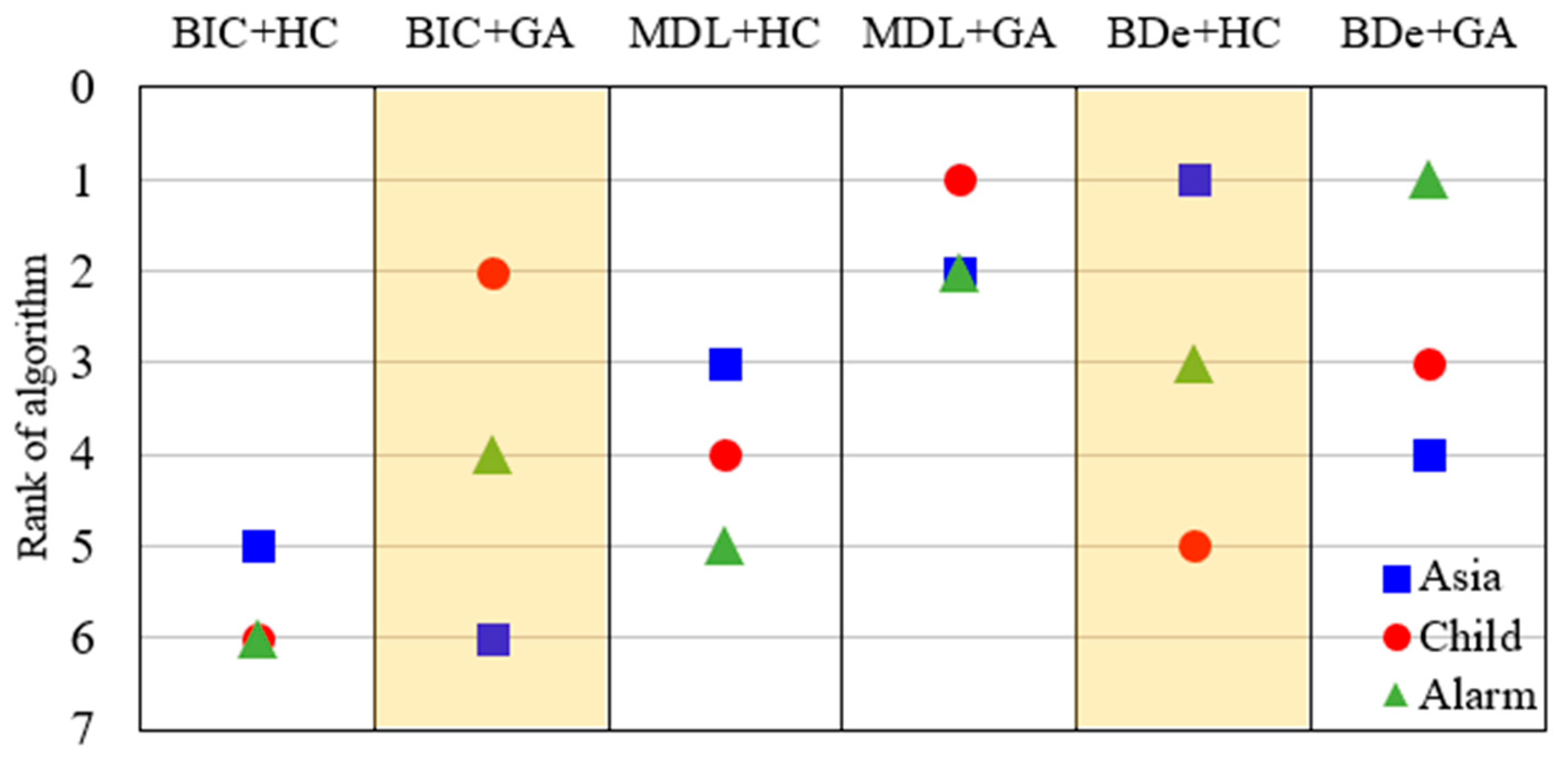
Figure 2.
Algorithm process of C-EL.
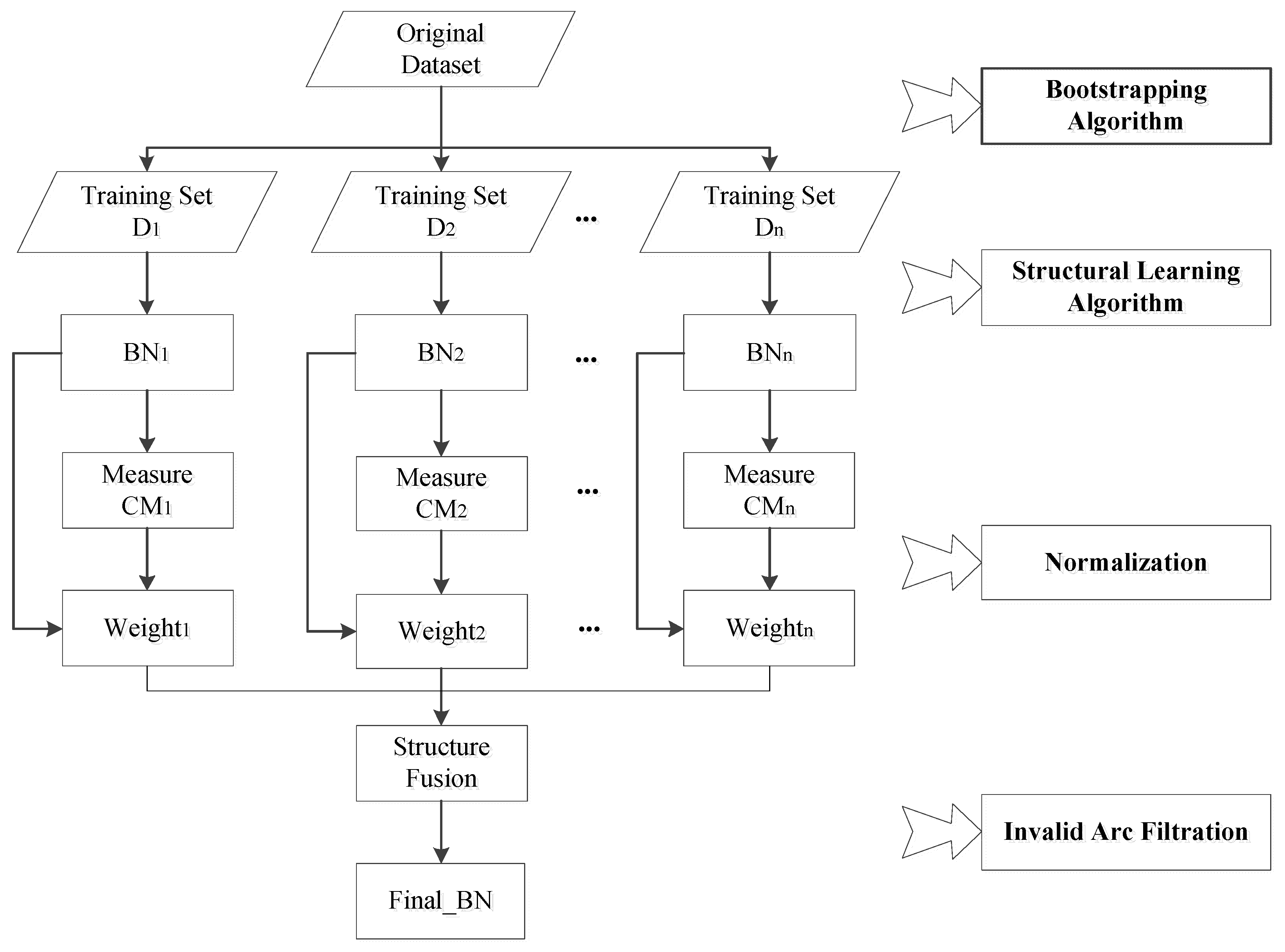
Figure 3.
Adjacency matrixes of Asia based on different structural learning algorithms.
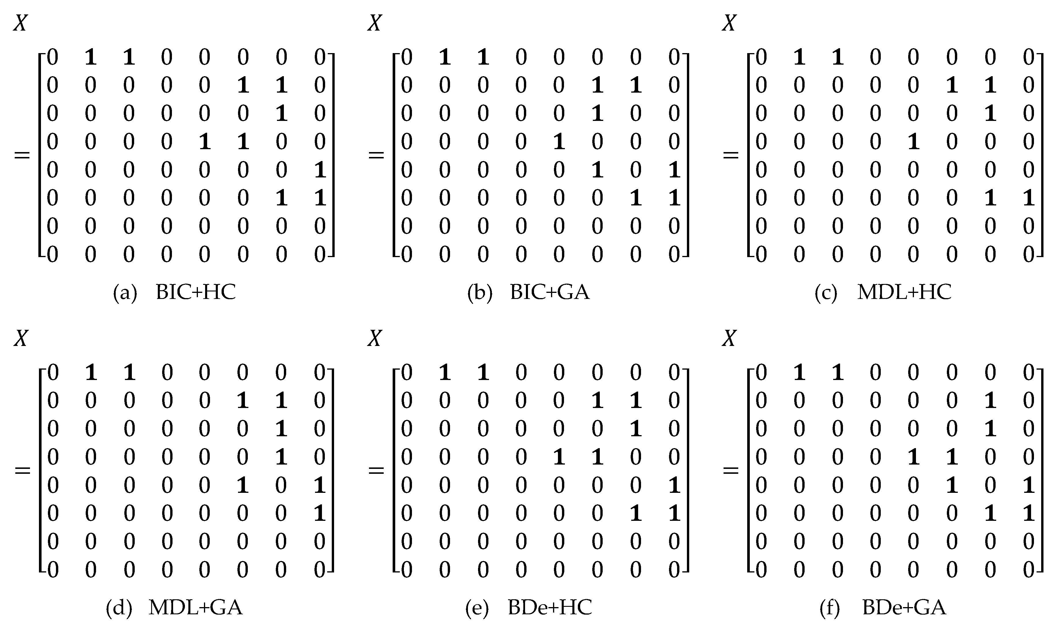
Figure 4.
Causal transition matrix and adjacency matrix of Asia.
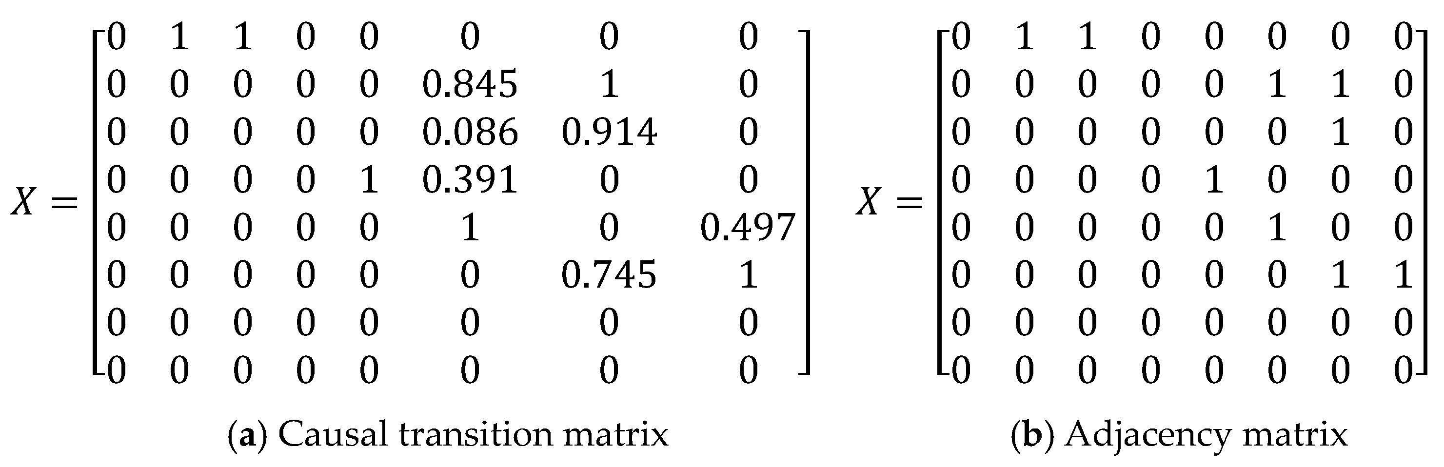
Figure 5.
Learning structure and actual structure of Asia.
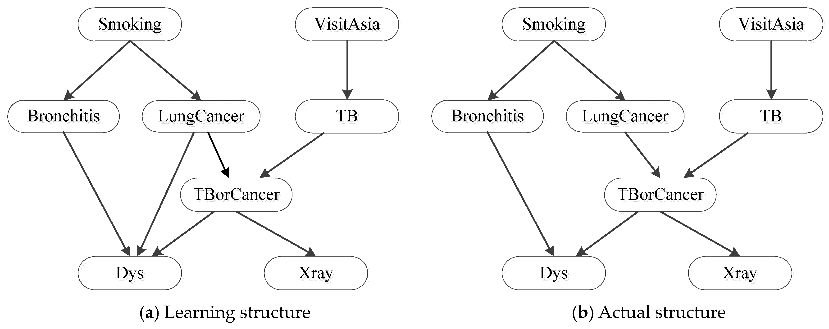
Figure 6.
Results of all evaluation indexes of three BNs with different algorithms.
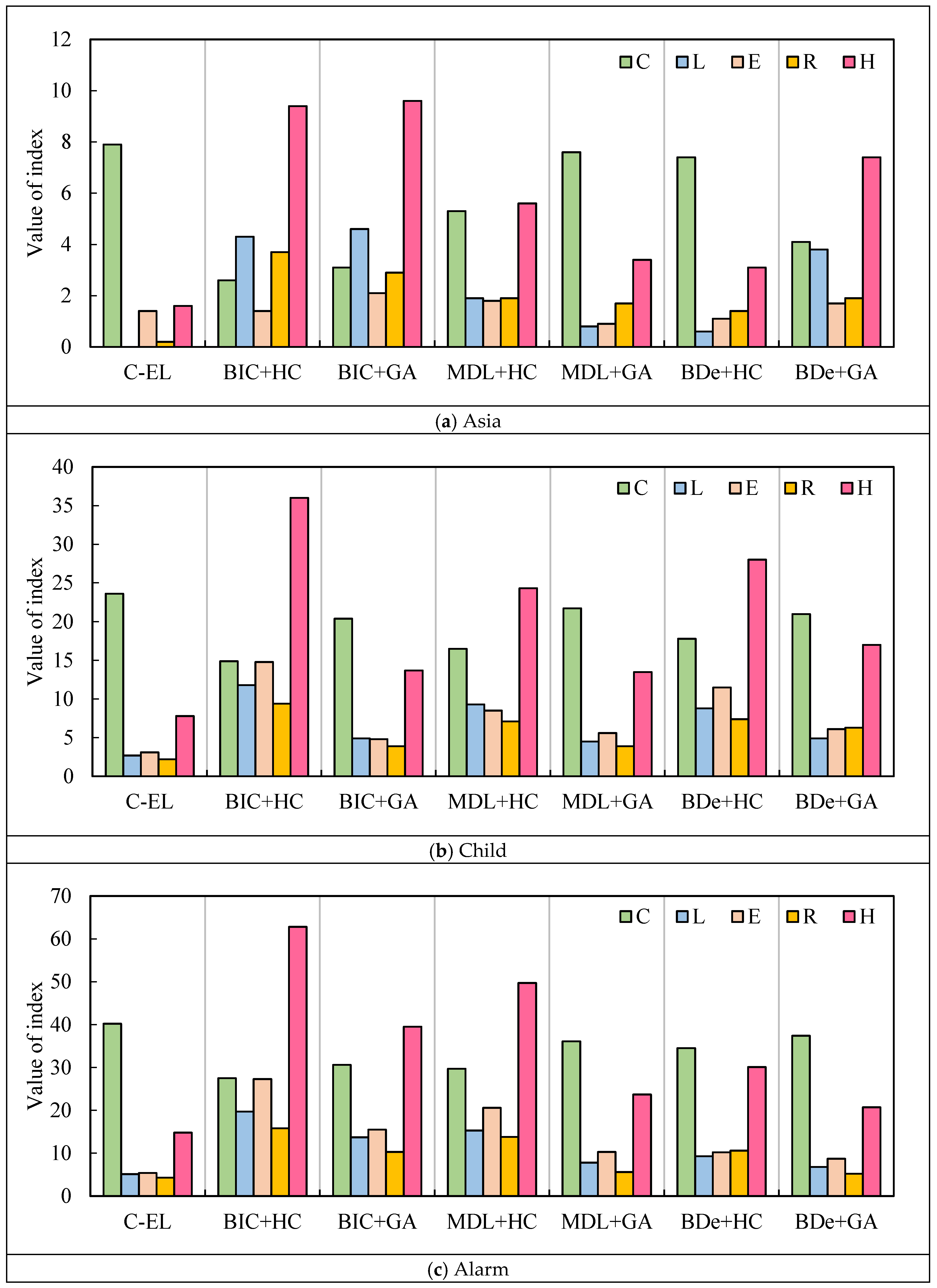
Figure 7.
of three BNs with different algorithms and sample sizes.
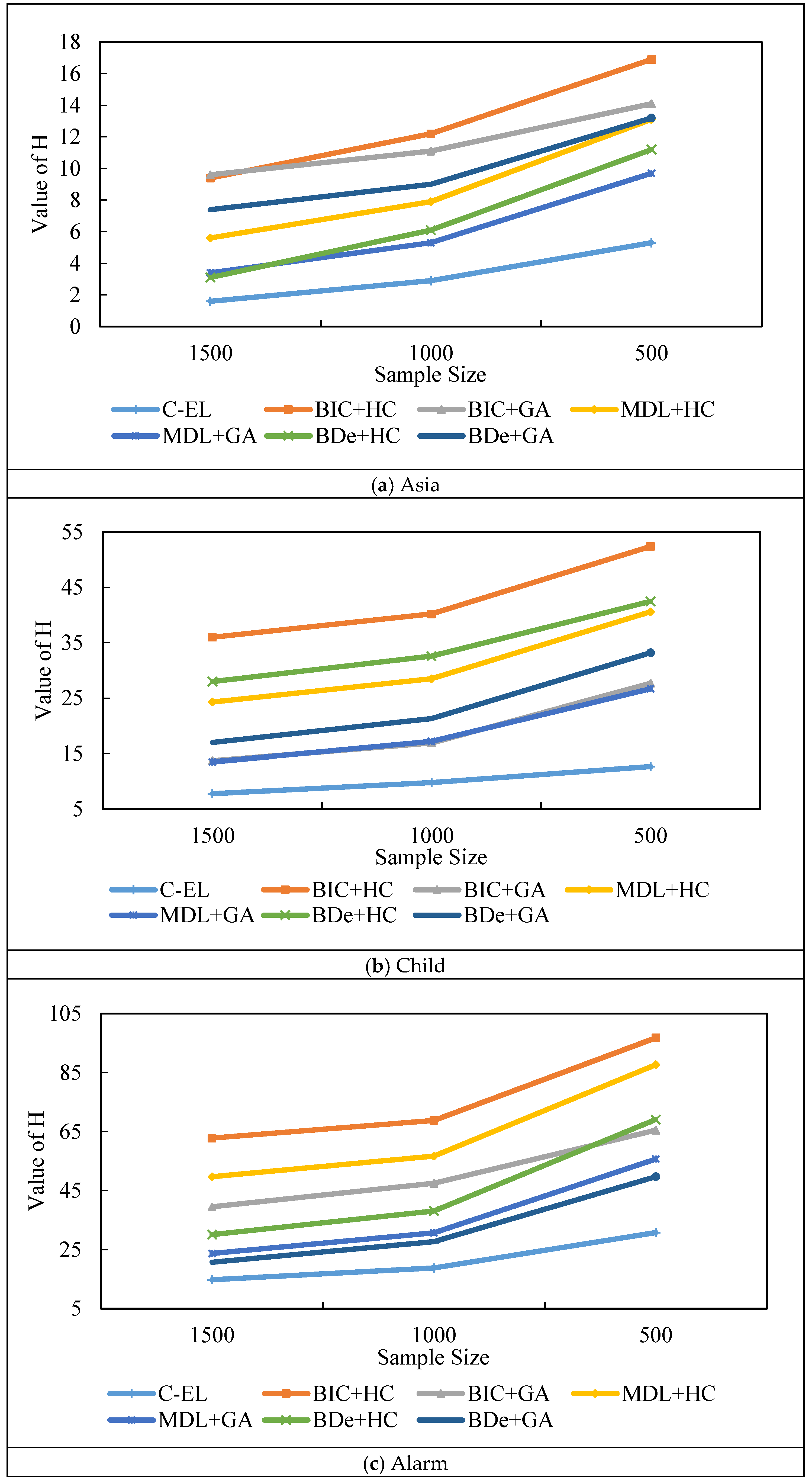
Figure 8.
Change of Hamming distance of three BNs with threshold value.


Table 1.
Training datasets of the Asia network.
| Node | Smoking | Bronchitis | LungCancer | VisitAsia | TB | TBorCancer | Dys | Xray |
|---|---|---|---|---|---|---|---|---|
| Sample 1 | 2 | 2 | 1 | 1 | 1 | 1 | 2 | 1 |
| Sample 2 | 1 | 1 | 1 | 1 | 1 | 1 | 1 | 1 |
| Sample 3 | 1 | 1 | 1 | 1 | 1 | 1 | 1 | 1 |
| Sample 4 | 2 | 2 | 1 | 1 | 1 | 1 | 1 | 2 |
Table 2.
Mean of three Bayesian Networks (BNs) with different Search-Score (SS) algorithms (the numbers in brackets represent the ranking).
Table 2.
Mean of three Bayesian Networks (BNs) with different Search-Score (SS) algorithms (the numbers in brackets represent the ranking).
| SS Algorithm | Asia | Child | Alarm |
|---|---|---|---|
| BIC + HC | 8.3 (5) | 14.7 (6) | 68.2 (6) |
| BIC + GA | 10.4 (6) | 8.1 (2) | 39.1 (4) |
| MDL + HC | 5.9 (3) | 11.2 (4) | 52.7 (5) |
| MDL + GA | 5.1 (2) | 6.8 (1) | 25.4 (2) |
| BDe + HC | 3.2 (1) | 12.9 (5) | 31.2 (3) |
| BDe + GA | 7.6 (4) | 10.4 (3) | 17.6 (1) |
Table 3.
Causal Information Flow (IF) between every two nodes in Asia.
| Smoking | Bronchitis | LungCancer | VisitAsia | TB | TBorCancer | Dys | Xray | |
|---|---|---|---|---|---|---|---|---|
| Smoking | \ | 0.0109 | 0.0154 | −0.0021 | 0.0002 | 0.0152 | 0.0216 | 0.0042 |
| Bronchitis | −0.0131 | \ | 0.0030 | 0.0003 | 0.0037 | 0.0028 | 0.0332 | 0.0009 |
| LungCancer | 0.0076 | 0.0062 | \ | 0.0008 | 0.0001 | −0.6909 | 0.0152 | 0.0312 |
| VisitAsia | 0.0026 | 0.0018 | 0.0012 | \ | 0.0243 | 0.0014 | −0.0127 | 0.0025 |
| TB | −0.0087 | −0.0059 | 0.0010 | 0.0001 | \ | 0.0008 | −0.0060 | 0.0014 |
| TBorCancer | 0.0274 | 0.0056 | −0.6909 | 0.0015 | 0.0026 | \ | 0.0160 | 0.0321 |
| Dys | 0.0087 | −0.0320 | 0.0044 | 0.0029 | 0.0009 | 0.0041 | \ | 0.0078 |
| Xray | 0.0323 | 0.0011 | −0.0530 | 0.0019 | 0.0014 | −0.0537 | 0.0211 | \ |
Table 4.
Causality measure and weight of three BNs with different SS algorithms.
| BN | Index | BIC + HC | BIC + GA | MDL + HC | MDL + GA | BDe + HC | BDe + GA |
|---|---|---|---|---|---|---|---|
| Asia | Causality Measure | 0.3557 | 0.3028 | 0.6332 | 0.8925 | 0.7723 | 0.5446 |
| Weight | 0.1016 | 0.0865 | 0.1809 | 0.2549 | 0.2206 | 0.1556 | |
| Child | Causality Measure | 2.0977 | 2.7955 | 2.6274 | 2.9059 | 2.4600 | 2.6893 |
| Weight | 0.1347 | 0.1795 | 0.1687 | 0.1866 | 0.1579 | 0.1727 | |
| Alarm | Causality Measure | 4.1490 | 4.4804 | 4.2021 | 4.8115 | 4.7294 | 5.0627 |
| Weight | 0.1512 | 0.1633 | 0.1532 | 0.1754 | 0.1724 | 0.1845 |
Table 5.
and of three BNs with different algorithms.
| Criteria | BN | C-EL | BIC + HC | BIC + GA | MDL + HC | MDL + GA | BDe + HC | BDe + GA |
|---|---|---|---|---|---|---|---|---|
| Asia | 7.9 | 2.6 | 3.1 | 5.3 | 7.6 | 7.4 | 4.1 | |
| Child | 23.6 | 14.9 | 20.4 | 16.5 | 21.7 | 17.8 | 21.0 | |
| Alarm | 40.2 | 27.5 | 30.6 | 29.7 | 36.1 | 34.5 | 37.4 | |
| Asia | 1.6 | 9.4 | 9.6 | 5.6 | 3.4 | 3.1 | 7.4 | |
| Child | 7.8 | 36.0 | 13.7 | 24.3 | 13.5 | 28.0 | 17.0 | |
| Alarm | 14.8 | 62.8 | 39.5 | 49.7 | 23.7 | 30.1 | 20.7 |
Table 6.
Rangeability of with variation of sample size.
| Algorithm | ΔH1500→1000 | ΔH1000→500 | ||||
|---|---|---|---|---|---|---|
| Asia | Child | Alarm | Asia | Child | Alarm | |
| C-EL | 1.3 | 2.0 | 4.0 | 2.4 | 2.9 | 12.1 |
| BIC + HC | 2.8 | 4.2 | 6.2 | 4.7 | 12.2 | 26.8 |
| BIC + GA | 1.5 | 3.2 | 7.9 | 3.0 | 10.8 | 28.4 |
| MDL + HC | 2.3 | 4.2 | 7.2 | 5.2 | 12.1 | 31.2 |
| MDL + GA | 1.9 | 3.7 | 7.4 | 4.4 | 9.5 | 24.7 |
| BDe + HC | 3.0 | 4.6 | 8.2 | 5.1 | 9.9 | 31.3 |
| BDe + GA | 1.6 | 4.3 | 6.9 | 4.2 | 11.9 | 21.8 |
Publisher’s Note: MDPI stays neutral with regard to jurisdictional claims in published maps and institutional affiliations. |
© 2020 by the authors. Licensee MDPI, Basel, Switzerland. This article is an open access article distributed under the terms and conditions of the Creative Commons Attribution (CC BY) license (http://creativecommons.org/licenses/by/4.0/).
Share and Cite
MDPI and ACS Style
Li, M.; Zhang, R.; Liu, K. A New Ensemble Learning Algorithm Combined with Causal Analysis for Bayesian Network Structural Learning. Symmetry 2020, 12, 2054. https://doi.org/10.3390/sym12122054
AMA Style
Li M, Zhang R, Liu K. A New Ensemble Learning Algorithm Combined with Causal Analysis for Bayesian Network Structural Learning. Symmetry. 2020; 12(12):2054. https://doi.org/10.3390/sym12122054
Chicago/Turabian StyleLi, Ming, Ren Zhang, and Kefeng Liu. 2020. "A New Ensemble Learning Algorithm Combined with Causal Analysis for Bayesian Network Structural Learning" Symmetry 12, no. 12: 2054. https://doi.org/10.3390/sym12122054
Note that from the first issue of 2016, this journal uses article numbers instead of page numbers. See further details here.