Smart Root Search (SRS): A Novel Nature-Inspired Search Algorithm

Abstract

In this paper, a novel heuristic search algorithm called Smart Root Search (SRS) is proposed. SRS employs intelligent foraging behavior of immature, mature and hair roots of plants to explore and exploit the problem search space simultaneously. SRS divides the search space into several subspaces. It thereupon utilizes the branching and drought operations to focus on richer areas of promising subspaces while extraneous ones are not thoroughly ignored. To achieve this, the smart reactions of the SRS model are designed to act based on analyzing the heterogeneous conditions of various sections of different search spaces. In order to evaluate the performance of the SRS, it was tested on a set of known unimodal and multimodal test functions. The results were then compared with those obtained using genetic algorithms, particle swarm optimization, differential evolution and imperialist competitive algorithms and then analyzed statistically. The results demonstrated that the SRS outperformed comparative algorithms for 92% and 82% of the investigated unimodal and multimodal test functions, respectively. Therefore, the SRS is a promising nature-inspired optimization algorithm.

1. Introduction

Nature is replete with intelligent and disciplined phenomena with impressive capabilities that are being continuously discovered. The behavior of animals and insects has been observed for centuries; however, the observed behaviors, which are represented by physics and particle dynamics, represent only a small portion of the intelligent processes that exist in nature. The intelligent behavior found in nature has inspired many intelligent search algorithms, such as genetic algorithms (GAs) [1], particle swarm optimization (PSO) [2,3], ant colony optimization [4,5], the artificial fish swarm algorithm [6], the artificial immune system [7], bacterial foraging optimization algorithm [8,9], bat-inspired algorithm [10,11], imperialist competitive algorithm [12,13,14], and the gravitational attraction search [15]. Although each of the intelligent search algorithms exhibits their own set of efficiencies and can solve many types of optimization problems, there are some issues they have in common for solving large-scale problems especially those possessing search spaces with staggering high dimensions. Amongst these issues, local optima problem [16,17,18] and the absence of inborn exploitation operations [19,20,21] are seemingly impossible to overcome. Thus, many researchers are searching for unique methods to tackle these issues. Hybrid heuristic search and memetic algorithms [19,22,23] have been proposing since years ago to tackle these problems. Innovative combinations of the Bee colony algorithm with other heuristics are also showing promising results in properly exploring search spaces [24,25].

In the process of searching the soil for nutrients, such as minerals and water, plant roots demonstrate highly intelligent behavior [26]. This intelligence must be creative to ensure the survival of the plant in environments with low levels of water and insufficient nutrients. In these limited-resource communities, roots, as explained in Section 1.1.1, often adapt and search a broad area before plant dies due to absence of food or water. Therefore, the intelligent behavior of roots could be the basis for a brand new, swift, effective, and appealing intelligent search algorithm able to efficiently search large spaces.

A few attempts have been made to imitate plant root behavior and develop new search algorithms. These studies resulted in four algorithms: the root growth model (RGM) [27], root mass optimization (RMO) [28], the artificial root foraging model (ARFO) [29,30] and artificial root mass (ARM) [31]. Despite researchers’ efforts, the proposed algorithms have been unable to utilize plant intelligence in a way that overcomes the weaknesses that affect other heuristic search algorithms (refer to Section 1.1.2 for more details).

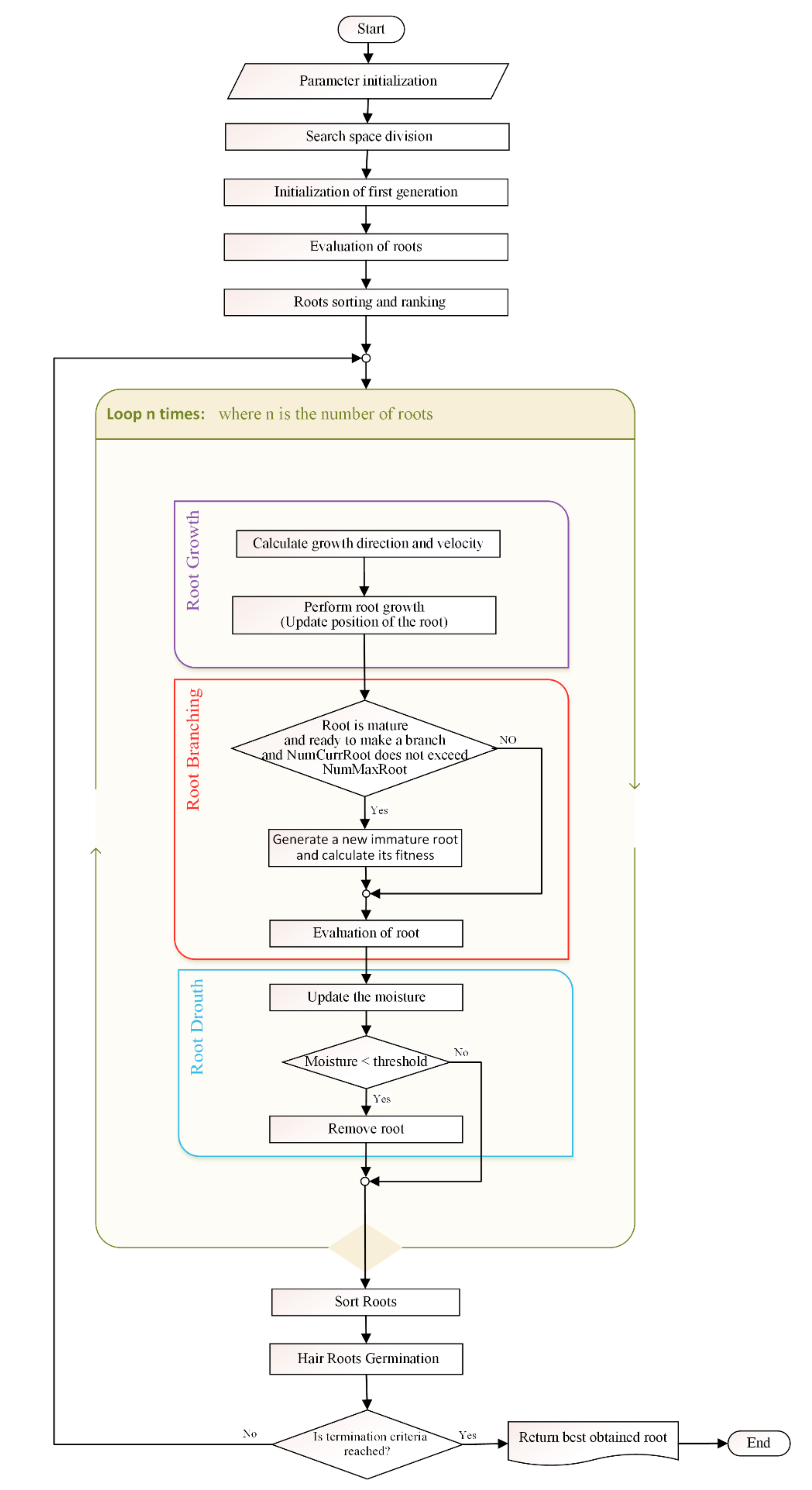
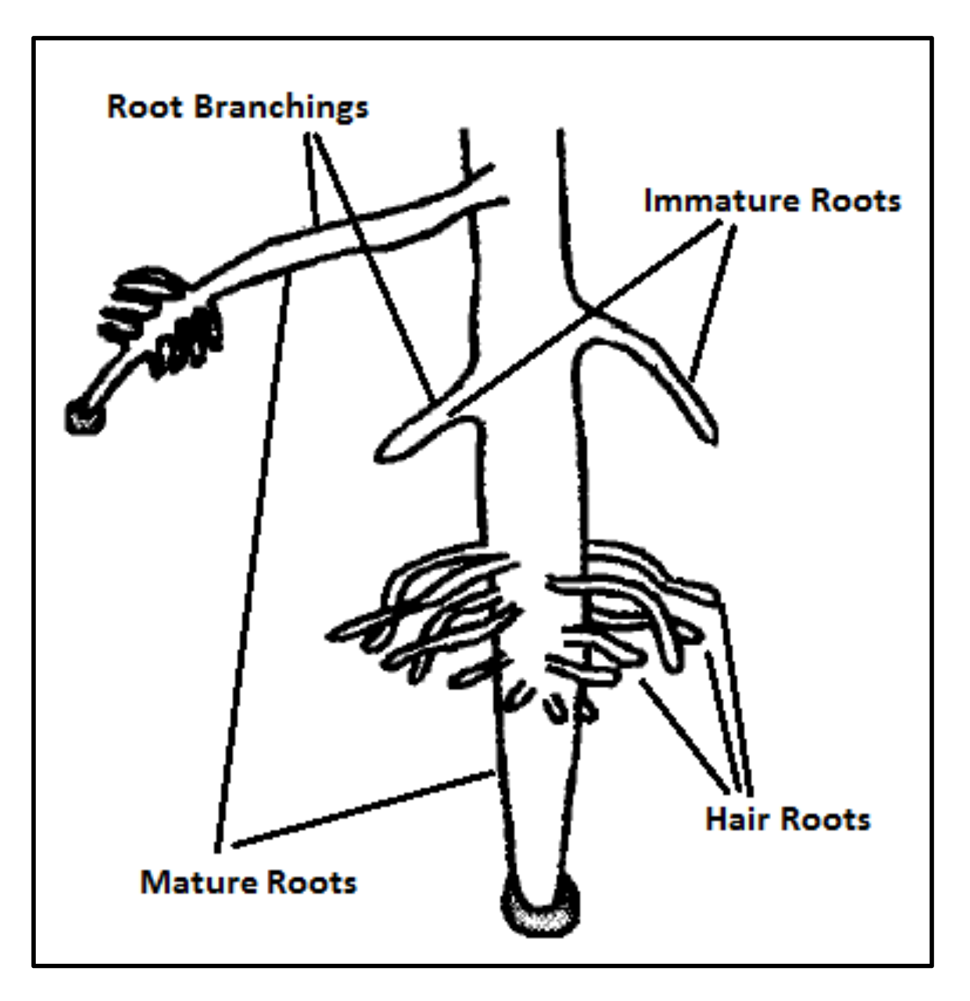
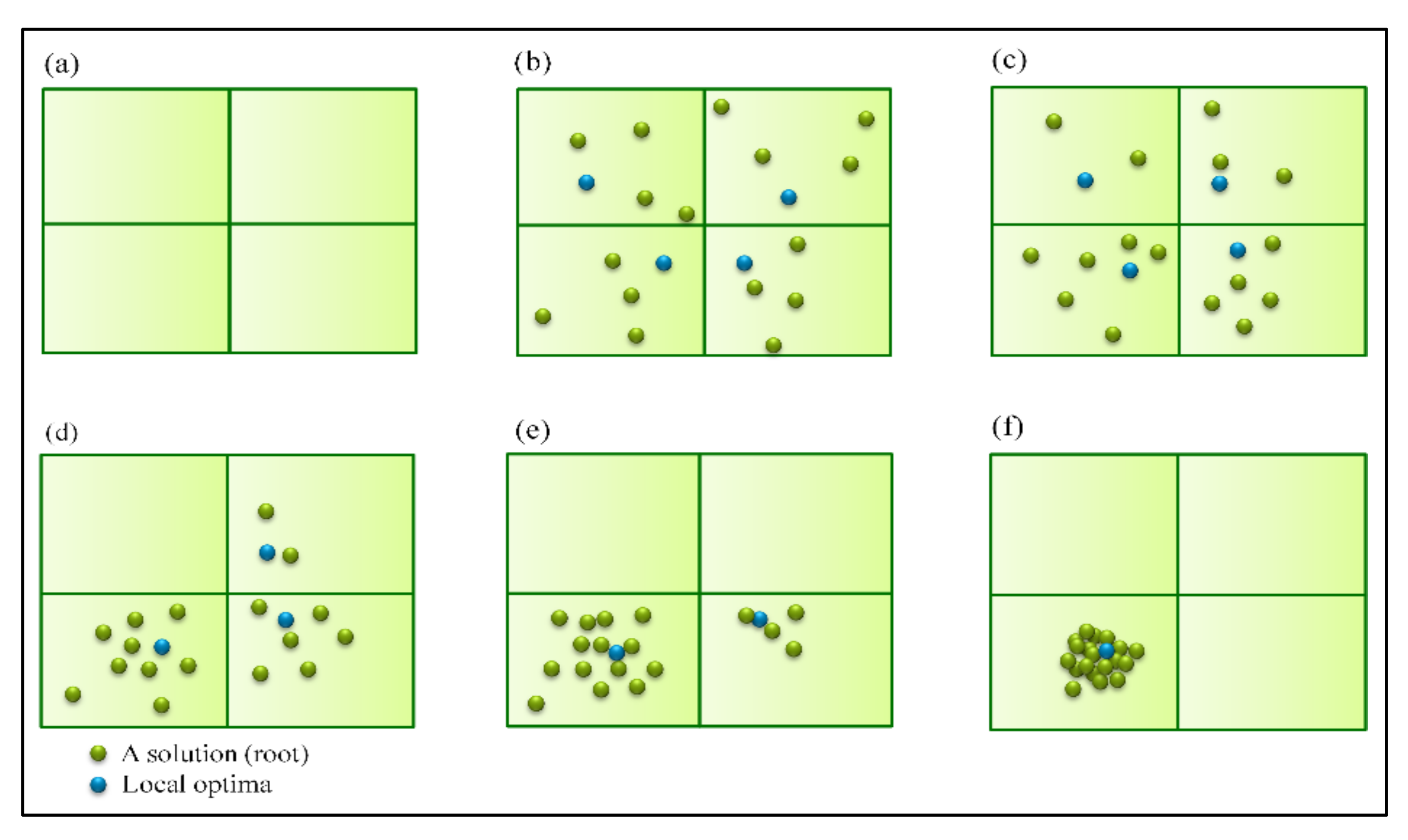
Hence, to achieve high efficiency and overcome problems, a new, independent, growth-inspired Smart Root Search (SRS) algorithm was proposed by the authors of this paper in [32]. The SRS is equipped with unique features and well-defined operators that are extracted precisely from intelligence of plant, and, unlike previous plant root-based search algorithms, is in absolute alignment with optimization principles. The novelty of SRS can be summarized in three items including (1) dividing the search space into a number of subspaces helping the algorithm to quickly find the more potential areas of the search space, and control local convergence of the algorithm in those areas; (2) defining three different types of roots, immature, mature and hair roots, that use different exploration approaches together with a mechanism to convert immature to mature, in order to search more in promising areas and provide embedded local search mechanism; and (3) proposing root drouth operator to control local and global convergence of the algorithm simultaneously.

As the proposed SRS was a brief preliminary model, it required supplementary parts, revision, implementation, test and comparison. To this end, in this paper the final version of the model is proposed and explained in detail and represented in the form of flowchart and pseudocode. Supported by graphical examples, a new structure is employed for roots for getting better performance, and root drought equation is improved to protect promising roots more accurately. In addition to that, a clear parameter initialization is added to the algorithm, and a precise explanation is provided for Immature-to-Mature mechanism of the roots. Most importantly, a complete experimental test has designed and applied to evaluate the performance of the algorithm and compare with introduced comparative algorithms followed by an in-detail statistical test.

The remainder of the paper is structured according to the following. The literature on the intelligent behavior of roots is reviewed in Section 1.1. A detailed explanation of the SRS algorithms is then described in Section 2, followed by the experimental test and results in Section 3. Finally, conclusion and suggestions for future work are provided in Section 4, followed by references.

1.1. Literature Review

From a general perspective, living things can be divided into two main groups: animals and plants. Animals sense their environment using their senses, such as sight and touch. Similarly, plants perceive their surrounding environment using a series of senses and reactions. To become more familiar with plant physiology and their senses and reactions, this section provides information on how plant roots sense their environment and the consequences of these reactions.

1.1.1. Plant Senses and Reactions

Plants use the same five senses as humans: hearing [33], touching, tasting, seeing and smelling. Furthermore, plants have evolved to use more senses than humans and, in fact, have approximately twenty distinct senses. Indeed, plants are able to detect moisture, gravity, minerals, humidity, light, wind, soil composition and structure, snow melt, pressure, temperature, and infection. Plants can decide to react against environmental stimuli based on the information obtained by these senses. Thus, plants are considered prototypical intelligent creatures [26,34] and exhibit their intelligence via shoot and root growth.

A thorough review on the architecture of root system and the pathways and networks forming root behavior was provided in [35]. Those authors showed that root growth is a reaction to the nutrients of the soil depending on several changing factors. Hydrotropism, nutrient tropism, cell memory and electrical impulse are some of the most interesting behaviors that demonstrate root intelligence. These behaviors are summarized below.

Hydrotropism: Plant survival depends on the ability of roots to find water in soil. Hence, plant root growth curves correspond to the moisture gradient (higher water potential) called hydrotropism [36,37].

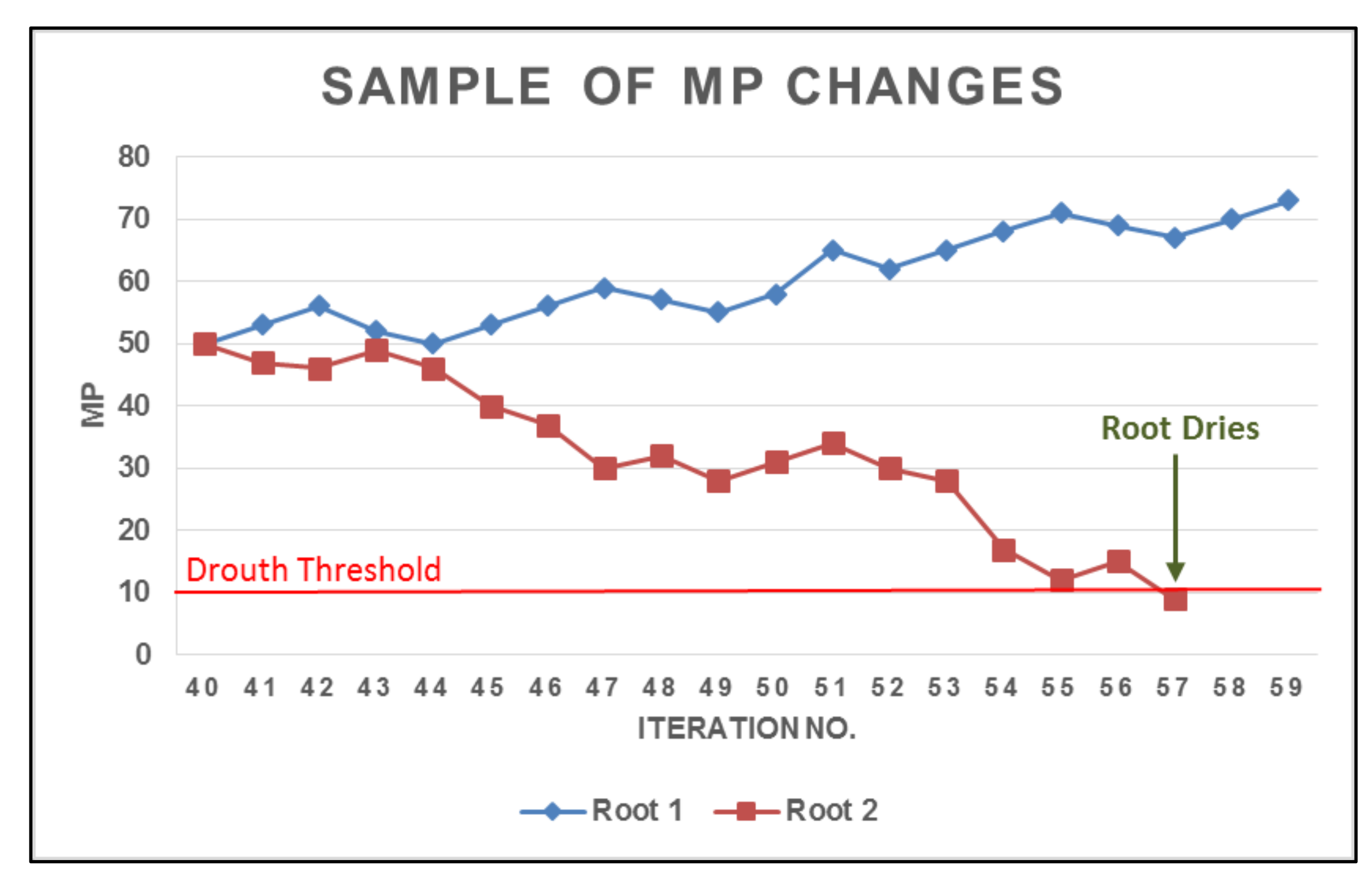
In addition, when they encounter moisture in soil, roots absorb and store water to support all plant activities. The plant loses stored water during plant growth or evapotranspiration. Roots can also transfer water to dry parts of the soil and release it to promote root survival [38,39,40]. This release occurs when the absorbed water is not sufficient for root survival because roots that cannot survive will dry out.

Nutrient tropism: Nitrates and phosphates are considered the most important elements for plant growth [41]. Important developmental processes, such as lateral root (LR) and hair root (HR) formation as well as primary root (PR) elongation (length), are to a great extent sensitive to the nutrient concentration changes.

Strong evidence shows that the nitrate concentration affects LR formation: development of LR is hindered by high nitrate concentrations and stimulated by low concentrations of nitrate, respectively [35,42]. PR elongation under the inhibitory impact of high nitrate concentrations is also discussed in [43]. Accessibility and distribution of phosphate and Nitrate have been shown to have contrasting effects on PR elongation and LR density but comparable impacts on LR elongation [44]. PR elongation is known to decrease with increasing nitrate availability but increase as the phosphate supply increases. The LR density remains constant across varying concentrations of nitrates but decreases as the phosphate supply increases. In contrast, LR elongation is suppressed by high concentrations of nitrate as well as phosphate.

In this regard, Ref. [45] demonstrated that phosphate starvation enhances HR elongation and density. Furthermore, research conducted at the Pennsylvania State University shows that Arabidopsis thaliana roots grow more condensed and longer reacting to lower availability of phosphate [46].

Memory: Although plants do not have a neural network, many studies show that they can recall some conditions, which suggests that plants exhibit memory. Ref. [47] addressed traumatic plant memories, related facts, and potential mechanisms. Stress factors make the plant impervious to subsequent exposures. This stress-related feature indicates that every plant has a memory capacity. In addition, plants also possess “stress memory” and “drought memory”. Surprisingly, the proportion of live biomass after a late drought is higher in plants that were exposed to drought earlier in their growing season contrasted with single-stressed plants [48].

Electrical Impulse: Plants also use a message-passing system [49]. Research on plants has shown that electrical communication plays a significant role in root-to-shoot contact in the plants under water stress. Furthermore, Ref. [50] showed that when one organ of a seedling is stimulated (i.e., the root region), a characteristic response (electrical stimulus) is produced and would be recorded upward in another organ from the stimulating area.

1.1.2. Plant-Imitating Methods

A comprehensive analysis at plant root domains shows that only a few research studies have focused on using the inherent intelligence of the plants as a search algorithm. The studies have been leaded and conducted by Zhu Yunlong and his several research teams, respectively. In this section, the small number of proposed plant root algorithms and the main ideas are assessed and discussed.

RGM is a proposed algorithm for numerical function optimization that simulates the interactions between HR growth and the soil [27,51]. In each iteration of growth in RGM, high-functioning roots, which have higher Morphactin (fitness function) values, are selected to branch areas distant from the selected roots. New branches are called HRs. HRs follow random growth directions, and their growth length depends on their growth direction. HRs are added to a set of roots, and then a set of non-selected branching roots is removed. Accordingly, RGM could be known as a local search algorithm that does not take advantage of the well-extracted root intelligence and is not suitable to search in large search spaces. Furthermore, when local optima become trapped, the RGM method fails.

In 2013, an RGM for numerical optimization—the RMO algorithm—was proposed [28]. RMO is the primary inspiration for two other algorithms: ARFO and ARM.

ARFO [29,30] was proposed for image segmentation problems and then generalized to address other optimization problems. This algorithm uses the Auxin hormone levels of roots as the objective function and employs branching, re-growing, hydrotropism and gravity-tropism operations. The ARFO root system consists of three groups of roots, including main roots and lateral roots (large and small elongated length units, respectively) and dead roots. Two main shortcomings of ARFO are evident: first, absence of precise extraction and accurate modeling of plant intelligence in terms of root growth. Second, optimization-averse behavior is inherent in the algorithm. A list of shortcomings of the ARFO is presented in

Table 1. Intelligent and optimization-averse behaviors of artificial root foraging model (ARFO) algorithm.

Optimization-Adversative Behaviors	Common Intelligent Behaviors
Increasing root length in promising main root areas	Using short-step movements/changes in promising areas to identify additional search locations
Decreasing root length in non-promising LR areas	Using large-step movements/changes in non-promising areas to escape non-promising areas
LR are exploited in non-promising areas	Exploitation occurs in promising areas
Applying short-length branches causes very fast convergence	Avoiding fast convergence
No chance for enhancing bad solutions	Bad solutions have more chances for enhancement

.

ARM optimization was proposed to solve the data clustering problem. ARM is based on a harmony-like search algorithm [52] that simulates plant root growth strategies, such as proliferation and decision making, that depend on the growth direction [31]. ARM generates a set of roots randomly. Some of the roots with better fitness values can continue their growth, while the rest stop growing. For every root, one neighbor is selected randomly. If the fitness of the neighbor is better than that of the root, then a new root will be generated between them in the search space; otherwise, a new root will be generated randomly. The new root will be added to the set of roots with better fitness values than its parent. Therefore, no intelligent root behaviors are applied in ARM.

2. Smart Root Search Algorithm

2.1. Intelligence of Plant Root Growth

Root growth intelligence can be outlined as follows:

(a)

Roots grow in the direction of the nutrient sources in the soil.

(b)

Root growth accelerates and generates new branches and HRs depending on the nutrient concentration of the soil.

(c)

Each part of a root uses electrical impulses to send information about its current situation to the other parts.

(d)

Plants can memorize and respond to information.

(e)

Water stress states cause roots to dry up.

These intelligence mechanisms motivated us to design the SRS optimization algorithm. The SRS is described in detail in Section 2.2.

Table 2. Mapping optimization terms and plant root mechanism.

Botany Terms	Optimization Terms
Soil	Search Space
Plant Root Set	Solutions’ Vector
Root	Solution
Nitrate Concentration	Objective Function
Location of the Highest Nitrate Concentration	Optimal Solution
Growth Step	Iteration
Hair Roots Germination	Local Search Operator
Root Growth	Solution Movement
Root Drouth	Solution Elimination
Root Growth Speed	Velocity of Movement
Branching	Solution Reproduction
Immature Root	Limited-move Solution
Growth Direction	Movement Coefficient Set

presents a mapping of the optimization with real plant root growth (botany) terms.

2.2. SRS Algorithm

The SRS has some characteristics that distinguish it from similar algorithms.

• SRS divides the search space into several subspaces and distributes the first generation of roots equally among them. This helps SRS to apply different search policies to different parts of the search space. Similar algorithms do not provide such functions in their standard versions.
• SRS-generated roots are immature upon germination but become mature after a few iterations. Thus, the algorithm can apply different search policies by using the same roots based on their age. In contrast, other algorithms use fixed exploratory policies during their execution.
• SRS utilizes an embedded local search mechanism applied by a group of roots called HRs.
• SRS utilizes a dynamic population size. This gives the SRS the capability to decrease the number of solutions in non-promising subspaces and to increase the number of solutions in promising areas.

Knowing that, the main procedures of the SRS algorithm are Parameter Initialization, Dividing the Search Space, Initialization of the First Generation, Evaluation, Sorting and Ranking of the Roots, Root Growth, Root Drouth and Root Branching followed by HRG and Termination Criteria that are described in the following sections and visualized in Figure 1. In addition, the time complexity of the algorithm is discussed in Appendix B.

2.2.1. Parameter Initialization

SRS search elements and operations can be adjusted by setting a few guiding parameters. The parameter values depend on the problem specifications. Studying and understanding these parameters and how they affect the algorithm are crucial for applying the algorithm successfully. The parameters are defined in Section 2.2.2, Section 2.2.3, Section 2.2.4, Section 2.2.5, Section 2.2.6, Section 2.2.7, Section 2.2.8 and Section 2.2.9 and initialized in Section 3.1.1 for the investigated test functions.

2.2.2. Dividing the Search Space

In extensive search spaces, search algorithms must probe into a huge number of space points. Total number of space points is considerably more than the number of initial solutions in the first iteration of running the algorithm. As the initial solutions of the algorithm generate randomly, the distribution of the solution in the search space is not often uniform throughout the search space, and therefore, the search space would not be inspected thoroughly.

Thus, based on a divide-and-conquer strategy [53], SRS algorithm divides the problem search space into Ns subspaces. The number of subspaces directly affects the SRS convergence speed. Therefore, an effective Ns initialization value depends on the problem specifications including the structure of the solutions, number of dimensions and sizes of the various search space dimensions. The user can use any approach to divide the search space such that the boundary of each subspace can be determined.

2.2.3. Initialization of First Generation

The SRS randomly generates NumMinRoot number of solutions for initial generation so that the number of solutions in every subspace is equal. If there are some remaining unassigned solutions, they will be randomly assigned to the subspaces. Every solution in the SRS is mapped to a root, and the location of root i in a D-dimensional problem search space is presented below (Equation (1)), where $x_i^d$ represents the location of root i in dimension d. A basic structure of a root is also illustrated in Figure 2. Once this step ends, all subspaces possess the same number of roots generated.

$$x_i=\left(x_i^1,x_i^2,\dots ,x_i^d,\dots ,x_i^D\right)$$

(1)

2.2.4. Evaluation of Roots

Nitrate is the most important factor of growth in plants, followed by phosphate [41]. Botany research has demonstrated that concentration of nitrate and phosphate play critical roles in the root growth speed, and the density of branches and HRs [35,41,44,45,46,54,55,56]. These roles are summarized in

Table 3. Nitrate and Phosphate effects on root behaviors.

Nutrients Concentration	Effects
	Root Growth Speed	Hair Roots Density	Branching Density
High Nitrate		Nothing	Nothing
Low Phosphate
Low Nitrate		Nothing	Nothing
High Phosphate

Represents Increasing and represents Decreasing.

. In terms of the similar effects of high nitrate and low phosphate concentration on root growth speed, an aggregated effect of nitrate and phosphate can be extracted from Table 3, as shown in

Table 4. Aggregated Nitrate and Phosphate effects on root behaviors.

Nutrients Concentration	Effects
	Root Growth Speed	Hair Roots Density	Branching Density
High Nitrate & Low Phosphate
Low Nitrate & High Phosphate

Represents Increasing and represents Decreasing.

. To simplify the proposed model, those combinations in which the nitrate and phosphate concentrations exert the same effects on root growth speed are considered. Due to the importance of the simplicity of the SRS model, we suppose that as the concentration of nitrate increases, the concentration of phosphate decreases (Equation (2)). This assumption facilitates defining the concepts that are more compatible with the terminology of the botany. Accordingly, as shown in Equation (3), the only nutrient that affects root life is nitrate, and the objective function (f(x)) value of each root is considered as the Nitrate Concentration of that root.

$$\mathrm{Nitrate}\mathrm{Concentration}=\frac{1}{\mathrm{Phosphate}\mathrm{Concentration}}.$$

(2)

$$f\left(x\right)=\mathrm{Nitrate}\mathrm{Concentration}$$

(3)

2.2.5. Root Sorting and Ranking

The SRS sorts its current roots at the end of initialization step as well as all execution iterations. It lets SRS identifying the best roots of every subspace, ranking each root in the root list, and locate the global best root at the top of the list of roots.

2.2.6. Root Growth

The roots of plants expand at varying rates and in various directions in order to locate richer areas of nutritional elements. In the same way, SRS roots grow (move) within the problem search space to find superior locations. This growth occurs at a predesignated velocity in a given direction. Therefore, the velocity and direction of every root must be determined beforehand. The root growth mechanism leads to a controlled local convergence in every subspace. Further details of the root growth are provided in Section 2.2.6.2 and Section 2.2.6.3

From lifetime standpoint, SRS divides roots into two groups: permanent and temporary roots. Permanent roots are immature and mature roots that are defined based on their age. These roots fall into a temporary root category known as JRs. Figure 3 depicts the types of roots in a plant.

2.2.6.1. Types of Roots

• Mature Roots

Mature roots can change their growth direction and velocity to improve exploration. Once a mature root reaches a good location in the search space, it reduces its growth speed to explore the area more efficiently in increments. Consistently, such roots attempt to escape poor locations by increasing their growth speed. In addition, mature roots also make new roots (i.e., by branching) to facilitate searching alternate locations and directions. Once a mature root creates a new branch, it becomes the parent root of that new branch. As will be explained in Section 2.2.7, when growing in relatively appropriate areas of the search space, a root will form additional new branches. Therefore, mature roots are very flexible and exhibit different intelligent behavior during the search process.

II.

Immature Roots

The second group of permanent roots consists of immature roots. These types of roots are not old enough to create new branches or make changes in their velocity and direction. Instead, they retain their original characteristics until transforming into mature ones. Therefore, every immature root can just receive velocity from the parent root. Immature roots also continue growing into the location of the parent based on random directions determined during germination. SRS utilizes immature roots to explore more of the search space that has not yet been reached. Accordingly, they play an important role in SRS by avoiding the trapping of local optima.

III.

HR

Exploitation is a searching mechanism that can be utilized dependently or through hybridization with exploration methods to efficiently search the neighborhoods of the best generated solutions [23,58,59]. Many searching methods do not have an exploiting operation built-in and an additional local search method is needed to construct a hybrid method [19]. In contrast, in its structure, SRS employs hair roots to incorporate a fast but efficient exploiting mechanism.

HRs are short in size and age in the nature [35,46]. These roots support mature roots to gather more water and nutrients while they are in a rich part of soil. The natural behavior is simulated by SRS by an operator called HRG. HRs play their exploitation role without having to make new branches or grow in the search space; thus, the HR velocity and direction are not well defined.

2.2.6.2. Growth of Mature Roots

Definition 1. 

Best Root Set (BRS).

In every subspace, the first k best roots of the subspace create the BRS. For doing that, k will be specified by utilizing “Roulette Wheel Selection via Stochastic Acceptance” [60]. Every root of the subspace grows to the nearest root of the BRS. For finding the best nearest root to root i, $densit{y}_{j,i}$ is defined for every root j in BRS. Equation (4) gives the $densit{y}_{j,i}$, where the dominator is the Euclidean distance between roots i and j, $N{C}_j$ is the nitrate concentration of root j, and $x_i^d$ and $x_j^d$ are the locations of roots i and j in dimension d, respectively.

$$densit{y}_{j,i}=\frac{N{C}_j}{\sqrt{{{\displaystyle \sum }}_{d=1}^D{\left(x_j^d-x_i^d\right)}^2}}$$

(4)

Therefore, among the BRS roots, root j is the best nearest root to root i, and $densit{y}_{j,i}$ is maximized (Equation (5)).

$$best\_closes{t}_i=\left\{j|densit{y}_{j,i}isMAX\right\}$$

(5)

• Velocity of Mature Roots

A user-defined maximum velocity, $v_{max},$ is used to be a baseline of calculating the velocity of mature roots. The velocity of roots cannot exceed $v_{max}$. Then, in accordance with the rank of every root among all roots, the velocity of the root is determined as a fraction of $v_{max}$, such that the velocity is lower with increasing rank. This policy helps roots located in promising areas to grow slower and achieve more precise exploration while forcing the rest of the roots to move away from non-promising areas. The velocity of root i can be obtained by Equation (6), where $glb\_ran{k}_i$ and NumCurrRoot are the global rank of root i and the number of roots that currently exist, respectively.

$$v_i\left(t\right)=v_{max}-\left[v_{max}\left(1-\frac{glb\_ran{k}_i}{NumCurrRoot}\right)\right]$$

(6)

II.

Direction of Mature Roots

For every dimension, a coefficient is required for the current velocity of the root to grow in the direction of its best closest root by applying a proper dimensional velocity. In addition, the coefficients should take values so that the growing root does not grow beyond the best closest one. To obtain these important movement coefficients, geometric relationships are helpful. Let the growth angle of root i toward its best, closest root best_closest, be $\theta$. The growth angle cosine of root i in dimension d, $cos{\theta }_i^d$, will be calculated simply by using Equation (7).

$$cos{\theta }_i^d=\frac{x_{best\_closest}^d-x_i^d}{\sqrt{{{\displaystyle \sum }}_{d=1}^D{\left(x_{best\_closest}^d-x_i^d\right)}^2}}$$

(7)

Therefore, assuming the current location and growth velocity of root i in dimension d are $x_i^d\left(t\right)$ and $v_i^d\left(t\right)$, respectively, the next location of the root will be determined by Equation (8), for which $v_i^d\left(t\right)$ should be calculated by (9). To make root growth easier to realize and apply, a complete example of how a mature root grows from its current location ($x_i\left(t\right)$) to its next location ($x_i\left(t+1\right)$) is presented in Appendix A.

$$x_i^d\left(t+1\right)=x_i^d\left(t\right)+v_i^d\left(t\right)$$

(8)

$$v_i^d\left(t\right)=[v_i\left(t\right)\times cos{\theta }_i^d]$$

(9)

2.2.6.3. Root Growth of Immature Roots

As mentioned in Section 2.2.6.1, immature roots are newborn roots that are unable to change their growth velocity and direction or to make new roots. Regarding their growth velocity, every immature root gets its parent root velocity and will follow the growth behavior of the parent. Additionally, growth occurs in a randomly selected direction. To this end, every immature root that is generated randomly selects a point in its related subspace and considers that point its best, closest root. Then, Equation (7) is utilized to set the coefficients and determine the growth direction. Similarly, Equations (8) and (9) are applied to obtain the dimensional velocities and new locations.

2.2.6.4. Immature to Mature Transformation Mechanism

By providing a glimpse of the independent and complementary roles played by different types of roots, the mechanisms of SRS reveal how important it is to define a mechanism that transforms an immature root into a mature one. A simple maturation mechanism is proposed in SRS. As shown in Figure 1, every root has an attribute called Age. Age is initialized as 0 once a new root is generated. In each iteration of the algorithm, the root’s Age increases by one. If Age value of any of the immature roots reaches a threshold, Mature_Age, status of the root changes to “mature”. Mature_Age should be defined by the user based on the adopted exploration and exploitation policy such that higher Mature_Age values correspond to more exploration and less exploitation.

2.2.7. Root Branching

Branching is a mechanism in root growth that produces new roots to increase the search rate in those parts of the soil that have not yet been investigated. Similarly, SRS utilizes a Branching operation that generates new immature roots in the search space. Every new generated root in its early stages is adjacent to a mature root which is considered its parent.

In plant roots, two to five branches exist in each centimeter, depending on the phosphate concentration [44]. For SRS, a mechanism was designed to allow better roots to generate more branches. In this mechanism, branching is intended to encourage mature roots in every iteration by granting two to five nitrate concentration-based scores. Therefore, each mature root will branch after several iterations if the sum of collected scores (SCS) meets Minimum Required Ability (MRA) that is a predefined threshold value. The MRA can be set dynamically throughout the execution of the algorithm or determined by a user; higher MRA values correspond to fewer newly generated roots. Once a root reaches MRA and generates a new root, the SCS resets to 0, and the scores are re-collected.

This mechanism divides all the available roots in every subspace into four groups, each of which corresponds to one of the values of the range [2,5]. To avoid generating many ungainly new roots, higher scores should be assigned to small portions of roots having higher nitrate concentrations. Equation (10) is solved and the obtained value is used to dedicate the minimum possible percentage of roots needed to achieve this aim. The percentages of roots that should be assigned to other groups will be obtained using the next coefficients provided in the equation.

Table 5. Root group scoring for branching.

	Coefficient	Ratio of Group Roots to All	Score
Group 1	1	1 × 6.66 = 6.66%	5
Group 2	2	2 × 6. 66 = 13.33%	4
Group 3	4	4 × 6. 66 = 26.66%	3
Group 4	8	8 × 6. 66 = 53.33%	2

presents the root-dedication percentages of groups and scores. Additionally, Figure 4 shows how two different roots behave when collecting scores to reach MRA and generate new branches when located in two different parts of the search space.

$$x+2x+4x+8x=100\Rightarrow x\cong 6.66$$

(10)

2.2.8. Root Drouth

In order to remove improper roots while the number of roots in the search space increases due to the branching operator, another operator is required. This operator must be designed such that the proportion of newly generated roots and removed roots gets controlled and global convergence of the algorithm is guaranteed. As this operator simulates the root drouth mechanism of roots, the same name is employed. To simplify describing the Root Drouth operator, a new term will be defined.

Definition 2. 

To implement the Root Drouth operator, every root gains a certain volume of moisture, Moisture Percentage (MP), at initialization. As a moderate value, MP is initially 50. Whereas the MP changes as a mature root grows, immature roots have constant MP values to help them sustain throughout pre-pubertal development.

As mentioned previously, botany research has demonstrated that plant roots absorb and store water from the areas in soil that contain higher level of moisture and transfer this stored water for use in drier areas [38,39,40]. Root drouth occurs provided that a root encounters dry soil that lacks a water supply. In the growth process of a root in SRS, MP increases as much as the Encourage_Value or decreases as much as the Penalty_Value if the root arrives at a location that is better than its current location or does not, respectively. If MP decreases to a predetermined drouth threshold, the root dries out. To clarify the drouth process, a comparative sample is presented in Figure 5. This figure shows how two different roots are penalized or encouraged after maturing in iteration 40.

Encourage_Value is a constant, however Penalty_Value varies in different subspaces depending on the subspace rank. Thus, weak subspaces possess higher Penalty_Values, and accordingly, SRS dries the roots of weak subspaces earlier. To this end, a maximum penalty rate is considered, called Max_Penalty. thereupon, the Penalty_Value of subspace j, $Penalty\_Valu{e}_j$, will be calculated using Equation (12) where j, is the index and also rank of the subspace among all available subspaces that are sorted according to their best root. Penalty_change is calculated using Equation (11), where Ns is the number of available subspaces, and the decimal parameter called Penalty_Rate has a value in the range [0, 1]. Penalty_Rate strongly affects the convergence speed of the algorithm and should be defined by the user with respect to the problem characteristics. Smaller values of the Penalty_Rate, smaller Penalty_values for strong subspaces, and higher values of Penalty_Rate, smaller differences between the Penalty_values of weak and strong subspaces. We note that the rank of the best root of a subspace in the list of all existing roots determines the rank of that subspace.

$$Penalty\_Change=\frac{Max\_Penalty\left(1-Penalty\_Rate\right)}{Ns}$$

(11)

$$Penalty\_Valu{e}_j=\left\{\begin{array}{cc}Max\_Penalty*Penalty\_Rate,\hfill & \hfill j=1\\ Penalty\_Valu{e}_{j-1}+Penalty\_Change,\hfill & \hfill otherwise\end{array}\right.$$

(12)

Although Root Branching and Drouth cooperate to control the number of available roots, the SRS will likely encounter an overloaded root set, leading to a slow down. Thus, an auxiliary control mechanism is needed to initiate branching. Here, NumMaxRoot is defined as a threshold for the maximum number of roots currently active in the search space. If the number of active roots reaches NumMaxRoot, which is defined by the user, none of the roots can generate a branch, even they are otherwise eligible to do so, until vacancies are produced by the drying out of deficient roots drying.

2.2.9. HRG

HRG consists of the five following steps that begin with determining the number of roots can generate HRs and end with growth of the parent toward the best neighbor location found by the HRs.

• A set of the best mature roots (let us call them m) of every subspace will be picked by “Roulette Wheel Selection via Stochastic Acceptance” (RWSSA) [60] for generating plenty of HRs in their neighborhood regions.
• A random number l in the range (1, a) will be generated, where a is the neighborhood radius defined by the user based on the problem characteristics.
• For every selected mature root i in step 1, RWSSA will be used to generate a random number k in the range (1, D).
  • k of D dimensions of root i will be selected randomly.
  • For every selected dimension d in 3.a, two new roots, $HR{1}_i^d=\left(x_i^1,x_i^2,\dots ,x_i^d+l,\dots ,x_i^D\right)$ and $HR{2}_i^d=\left(x_i^1,x_i^2,\dots ,x_i^d-l,\dots ,x_i^D\right),$ will be generated, and their nitrate concentration needs will be calculated.
• If $HR{j}_i^d$ is one of the generated HRs with the greatest nitrate concentration value among the other HRs and their parents, then the parent will grow to reach the location of $HR{j}_i^d$.
• The generated HRs are no longer required and will dry immediately.

There are two HRG points that must be clarified. First, based on the 3rd step in the HRG, the 2k HRs will be generated in the neighboring area of a selected mature root in a D-dimensional space. Accordingly, in every iteration, a total of 2mk HRs will be generated. Second, the best rate of executing the HRG (i.e., the so-called HRG Rate) can be predefined by the user or calculated dynamically. Finding the best HRG Rate requires new dependent research, which we suggest as a possibility for the future.

2.2.10. Termination Criteria

Consistent with all other heuristic search algorithms, SRS execution will be stopped if at least one of the following criteria is met: (1) reaching the expected solution or (2) exceeding the maximum number of iterations. Once the algorithm stops, the best-found root will be shown as the final result of the algorithm. The SRS pseudo code is represented in Figure 6.

2.2.11. On the Convergence of the SRS

All elements of a search algorithm should cooperate to provide an average convergence rate that is not too fast or slow to reach the global best solution [61,62]. The SRS mechanisms are designed so that convergence is supported by two different but complementary approaches. First, each subspace has a local convergence rate when roots converge toward a few of their best local solutions. Here, the aim is finding the local optimal solution of every subspace. Second, global convergence occurs when, in the execution process, the roots of worse existing subspaces dry out based on the dynamic punishment process explained in Section 2.2.7 until there is only one subspace remaining at the last iterations of the algorithm. Finally, the local convergence of the last subspace together with the root drouth process will be leading to the identification of the global optimal solution of the problem. Figure 7 simply illustrates how available roots in different subspaces converge to their corresponding local optima and consequently facilitate reaching global optima in the best subspace by drying all the roots in the other subspaces.

3. Experimental Test, Results and Discussion

3.1. Experimental Tests: SRS vs. GA, PSO, Independent Component Analysis (ICA) and Differential Evolution (DE)

This section presents the results obtained by the SRS while searching for the optimal solution of the test functions described in Section 3.1.2. Here, performance of SRS is analyzed and compared with that of the employed comparative algorithms. A standard SRS is presented, and standard versions of GA, PSO, ICA and DE are employed as comparative algorithms. The best solution reached by each algorithm, the standard deviations of different solutions achieved in different runs by every algorithm, and the rank of each among all comparative algorithms are presented in the tables prepared for every test function.

This section consists of three subsections that explain the experimental methodology and settings, test functions and their specifications, and obtained results.

3.1.1. Settings

All algorithms were implemented in Microsoft Visual C# .NET 2015. To provide fair conditions for all comparative algorithms, common parameters, such as population size and the total number of evaluations of the objective function, were chosen to be the same for each algorithm. Referring to [63], the population size was selected to be 125. The maximum number of evaluations of the objective function was 1,000,000 to allow all algorithms to achieve the best possible solution. The other parameters are given below:

For GA, second point crossover operation, which influences the variation in generations, with a rate of 0.85 was employed as recommended by [64]. Mutation operation, which controls genetic diversity, was also set to 0.01 based on [64].

In PSO, C1 and C2 are constant coefficients that change the weighting of personal and global experiences, respectively, and both were set to 2 in our experiments. The inertia weight that demonstrates how particles’ previous velocity influences the subsequent velocity, was chosen to be 0.9, as recommended by [65].

In ICA, the imperialist rate states how many countries will be selected as imperialists. In addition, the competition rate is the second parameter of ICA, and it determines number of times that imperialists participate in a competition to take the weakest colony of the weakest emperor. To follow the research methodology described by [22], the mentioned parameters were set to 10 and 15, respectively.

F is a constant that can be used to manipulate the differential variation between two solutions in DE. It was selected to be 0.5 in our setting. The crossover rate value, which controls the changes in the diversity of the population, was set to 0.9, as recommended by [66].

SRS has effective parameters in its different parts. Assigning proper values for or defining equations to calculate these parameters is outside of the scope of this paper and requires independent studies. Hence, in this study, constant values are given to these parameters, as shown in

Table 6. SRS parameters setting.

	Ns	NumMinRoot (Population Size)	NumMaxRoot	Vmax	MRA	Max_Penalty	Encourage_Value	Penalty_Rate	Mature_Age
Unimodal Functions	8	125	2000	0.33 * MDV	20	10	2	0.75	4
Multimodal Functions	8	125	2000	0.33 * MDV	20	10	2	0.15, 0.25	15

, where the MDV is the Max Domain Value of the problem. This table shows that the assigned values of the Mature Age and Penalty Rate parameters are different for unimodal and multimodal functions. Given that the risk of falling into the trap of local optima increases for multimodal functions as the number of dimensions increases, assigning higher and lower values to the Mature Age and Penalty Rate parameters relative to those used for unimodal functions helps the SRS to explore areas that are slightly more distant from the current regions of active roots more thoroughly. Reversing these assignments for unimodal functions improves the ability of SRS to perform more exploitation around current roots and thus find better solutions.

3.1.2. Benchmark Functions

Many benchmark test functions are presented in the literature that are designed to provide identical comparison environments to evaluate the performance of optimization algorithms [67,68,69,70,71]. As a common methodology, these test functions are being used to test and validate the performance and efficiency of new optimization algorithms. Most known test functions can be categorized into unimodal and multimodal groups. Compared to unimodal functions, which have one and only one optimal solution, multimodal test functions have a number of optimal solutions, including global and local ones, making them suitable to evaluate the ability of an algorithm to avoid becoming trapped in local optima. For multimodal test functions, if an algorithm has a poor exploration process that cannot search the whole search space efficiently, it will inevitably fall into the trap of local optima.

Among the many different test functions available, a set of 24 most common ones were chosen in this research for comparing the performance of the GA, PSO, ICA, DE and SRS. This set includes 12 unimodal ($f_1$–$f_{12}$) and 11 multimodal ($f_{13}$–$f_{23}$) functions, which are listed in

Table 7. Unimodal Test Functions.

No.	Function	D	Range	${\mathit{f}}_{\mathit{m}\mathit{i}\mathit{n}}$	Formulation
$f_1$	Cigar	30	[−100, 100]	0	$x_1^2+{10}^6{\displaystyle {\displaystyle \sum }_{i=2}^D}{x}_i^2$
$f_2$	Dixon-Price	30	[−10, 10]	0	${\left(x_1-1\right)}^2+{\displaystyle {\displaystyle \sum }_{i=2}^D}i{\left(2x_i^2-x_{i-1}\right)}^2$
$f_3$	Quartic	30	[−1.28, 1.28]	0	${\displaystyle {\displaystyle \sum }_{i=1}^D}i{x}_i^4+random\left[0,1\right)$
$f_4$	Rosenbrock	30	[−5, 5]	0	${\displaystyle {\displaystyle \sum }_{i=1}^{D-1}}100{\left(x_{i+1}-x_i^2\right)}^2+{\left(x_i-1\right)}^2$
$f_5$	Schwefel 1.2	30	[−100, 100]	0	${\displaystyle {\displaystyle \sum }_{i=1}^D}{\left({\displaystyle {\displaystyle \sum }_{j=1}^i}{x}_j\right)}^2$
$f_6$	Schwefel 2.22	30	[−100, 100]	0	${\displaystyle {\displaystyle \sum }_{i=1}^D}\left|x_i\right|+{\displaystyle {\displaystyle \prod }_{i=1}^D}\left|x_i\right|$
$f_7$	Schwefel 2.23	30	[−10, 10]	0	${\displaystyle {\displaystyle \sum }_{i=1}^D}{x}_i^{10}$
$f_8$	Sphere	30	[−100, 100]	0	${\displaystyle {\displaystyle \sum }_{i=1}^D}{x}_i^2$
$f_9$	Step	30	[−100, 100]	0	${\displaystyle {\displaystyle \sum }_{i=1}^D}{\left(\lfloor x_i+0.5\rfloor \right)}^2$
$f_{10}$	SumSquares	30	[−10, 10]	0	${\displaystyle {\displaystyle \sum }_{i=1}^D}i{x}_i^2$
$f_{11}$	Trid 10	10	$\left[-D^2,D^2\right]$	0	$210+{\displaystyle {\displaystyle \sum }_{i=1}^D}{\left(x_i-1\right)}^2-{\displaystyle {\displaystyle \sum }_{i=2}^D}{x}_i{x}_{i-1}$
$f_{12}$	Zakharov	10	[−5, 10]	0	${\displaystyle {\displaystyle \sum }_{i=1}^D}{x}_i^2+{\left(0.5{\displaystyle {\displaystyle \sum }_{i=1}^D}i{x}_i\right)}^2+{\left(0.5{\displaystyle {\displaystyle \sum }_{i=1}^D}i{x}_i\right)}^4$

Column D represents the number of dimensions of the problem search space.

and

Table 8. Multimodal Test Functions.

No.	Function	D	Range	${\mathit{f}}_{\mathit{m}\mathit{i}\mathit{n}}$	Formulation
$f_{13}$	Ackley	30	[−32, 32]	0	$20+e-20e^{\left(\sqrt[-0.2]{\frac{1}{D}{{\displaystyle \sum }}_{i=1}^D{x}_i^2}\right)}-e^{\frac{1}{D}{{\displaystyle \sum }}_{i=1}^D\cos \left(2\pi x_i\right)}$
$f_{14}$	CosineMixture	30	[−500, 500]	0	$\mathrm{D}\times 1.643788341-0.1{\displaystyle {\displaystyle \sum }_{\mathrm{i}=1}^{\mathrm{D}}}\cos \left(5{\mathsf{\pi }\mathrm{x}}_{\mathrm{i}}\right)-{\displaystyle {\displaystyle \sum }_{\mathrm{i}=1}^{\mathrm{D}}}{\mathrm{x}}_{\mathrm{i}}^2$
$f_{15}$	Griewank	30	[−600, 600]	0	$\frac{1}{4000}\left({\displaystyle {\displaystyle \sum }_{\mathrm{i}=1}^{\mathrm{D}}}{\mathrm{x}}_{\mathrm{i}}^2\right)-\left({\displaystyle {\displaystyle \prod }_{\mathrm{i}=1}^{\mathrm{D}}}\cos \left(\frac{{\mathrm{x}}_{\mathrm{i}}}{\sqrt{\mathrm{i}}}\right)\right)+1$
$f_{16}$	Perm	4	[−D, D]	0	${\displaystyle {\displaystyle \sum }_{i=1}^D}{\left({\displaystyle {\displaystyle \sum }_{j=1}^D}\left(j^i+\beta \right)\left({\left(\frac{x_j}{j}\right)}^i-1\right)\right)}^2,\left(\beta >0\right)$
$f_{17}$	Qing	30	[−10, 10]	0	${\displaystyle {\displaystyle \sum }_{i=1}^D}{\left(x_i^2-i\right)}^2$
$f_{18}$	Quintic	30	[−1, 1]	0	${\displaystyle {\displaystyle \sum }_{i=1}^D}\left|x_i^5-3x_i^4+4x_i^3+2x_i^2-10x_i-4\right|$
$f_{19}$	Rastrigin	30	[−5.12, 5.12]	0	${\displaystyle {\displaystyle \sum }_{i=1}^D}\left(x_i^2-10\cos \left(2\pi x_i\right)+10D\right)$
$f_{20}$	Schwefel	30	[−500, 500]	0	$D\times 418.9829+{\displaystyle {\displaystyle \sum }_{i=1}^D}-x_i\sin \left(\sqrt{\left|x_i\right|}\right)$
$f_{21}$	Schwefel 2.25	30	[0, 10]	0	${\displaystyle {\displaystyle \sum }_{i=2}^D}\left[{\left(x_i-1\right)}^2+{\left(x_1-x_i^2\right)}^2\right]$
$f_{22}$	Styblinski_Tang	30	[−5, 5]	0	$D\times 39.16599+\frac{1}{2}{\displaystyle {\displaystyle \sum }_{i=1}^D}\left(x_i^4-16x_i^2+5x_i\right)$
$f_{23}$	Xin-She Yang 02	30	[−2π, 2π]	0	$\frac{{{\displaystyle \sum }}_{i=1}^D\left|x_i\right|}{exp\left({{\displaystyle \sum }}_{i=1}^D\sin \left(x_i^2\right)\right)}$

Column D represents the number of dimensions of the problem search space.

, respectively. The dimensions (D), domain ranges (Range), minimum value ($f_{min}$) and formulations of the employed test functions are listed in the mentioned tables.

3.2. Obtained Results and Discussion

The SRS and all comparative algorithms were repeated 40 times to solve every test function by employing different seed values. As all investigated test functions are minimization problems, the minimum objective function values obtained at the end of every execution were used to calculate the average value of obtained results (mean) and standard deviation (Std) of the results of the algorithms. The obtained mean values were also used to determine the ranks of the algorithms for different test functions. The mean and standard deviation of unimodal and multimodal function values obtained by GA, PSO, ICA, DE and SRS are shown in

Table 9. Comparison of SRS with GA, PSO, ICA and DE on Unimodal test functions. All results have been averaged over 40 runs.

No.	Function	GA		PSO	ICA	DE	SRS
${\mathit{f}}_{\mathit{1}}$	Cigar	Mean	6.62 × 108	1.12 × 109	8.44 × 108	9.33 × 108	1.11 × 107
		Std	2.51 × 108	1.5 × 108	4.93 × 108	1.37 × 109	2.62 × 106
		Rank	2	5	3	4	1
${\mathit{f}}_{\mathit{2}}$	Dixon-Price	Mean	677.43	276.84	2330.86	900.74	1.73
		Std	420.64	86.26	2929.02	1330.92	0.63
		Rank	3	2	5	4	1
${\mathit{f}}_{\mathit{3}}$	Quartic	Mean	18.88	11.94	11.03	9.53	14.003
		Std	2.91	0.78	0.64	0.29	1.4
		Rank	5	3	2	1	4
${\mathit{f}}_{\mathit{4}}$	Rosenbrock	Mean	528.93	437.82	545.02	258.45	25.55
		Std	315.32	106.66	418.31	139.21	2.85
		Rank	4	3	5	2	1
${\mathit{f}}_{\mathit{5}}$	Schwefel 1.2	Mean	37,415.48	7301.03	1652.85	1109.23	883.58
		Std	9582.99	1350.01	520.67	730.18	204.17
		Rank	5	4	3	2	1
${\mathit{f}}_{\mathit{6}}$	Schwefel 2.22	Mean	94.55	236.15	60.625	85	21
		Std	14.01	15.89	22.01	56.19	3.96
		Rank	4	5	2	3	1
${\mathit{f}}_{\mathit{7}}$	Schwefel 2.23	Mean	25.05	7.48	5127.09	104,269.3	0
		Std	46.41	4.46	11,643.33	542,120.6	0
		Rank	3	2	4	5	1
${\mathit{f}}_{\mathit{8}}$	Sphere	Mean	885.05	3195.13	800.43	727.2	11.75
		Std	287.48	525.35	395.63	1287.79	2.8
		Rank	4	5	3	2	1
${\mathit{f}}_{\mathit{9}}$	Step	Mean	811.78	3227.32	921.43	760.93	11.78
		Std	315.9	399.79	569.69	1298.97	2.96
		Rank	3	5	4	2	1
${\mathit{f}}_{\mathit{10}}$	SumSquares	Mean	104.36	74.59	125.65	107.42	0.52
		Std	40.67	16.14	43.7	136	0.31
		Rank	3	2	5	4	1
${\mathit{f}}_{\mathit{11}}$	Trid 10	Mean	454.98	22.78	133.88	95.05	2.88
		Std	444.18	13.52	68.36	215.89	8.8
		Rank	5	2	4	3	1
${\mathit{f}}_{\mathit{12}}$	Zakharov	Mean	58.9	0.032	2.31	1.28	0.003
		Std	27.98	0.01	2.04	3.31	0.002
		Rank	5	2	4	3	1

and

Table 10. Comparison of SRS with GA, PSO, ICA and DE on Multimodal test functions. All results have been averaged over 40 runs.

No.	Function		GA	PSO	ICA	DE	SRS
${\mathit{f}}_{\mathit{13}}$	Ackley	Mean	7.88	5.64	8.67	10.43	0.64
		Std	0.79	0.36	1.21	1.47	0.16
		Rank	3	2	4	5	1
${\mathit{f}}_{\mathit{14}}$	CosineMixture	Mean	2.993	2.999	3.296	2.978	2.975
		Std	0.019	0.016	0.063	0.015	0
		Rank	3	4	5	2	1
${\mathit{f}}_{\mathit{15}}$	Griewank	Mean	6.43	10.61	13.38	6.7	0.99
		Std	1.65	1.83	6.27	4.16	0.05
		Rank	2	4	5	3	1
${\mathit{f}}_{\mathit{16}}$	Perm	Mean	4.941	0.057	0.286	0.292	0.012
		Std	10.35	0.075	0.19	1.16	0.017
		Rank	5	2	3	4	1
${\mathit{f}}_{\mathit{17}}$	Qing	Mean	3.29 × 107	8.71 × 107	3.02 × 108	2.38 × 108	2.67 × 103
		Std	2.91 × 107	3.50 × 107	2.83 × 108	4.47 × 108	4.90 × 102
		Rank	2	3	5	4	1
${\mathit{f}}_{\mathit{18}}$	Quintic	Mean	50.4	86.05	149.16	63.38	15.91
		Std	9.33	8.69	84.74	63.89	5.02
		Rank	2	4	5	3	1
${\mathit{f}}_{\mathit{19}}$	Rastrigin	Mean	46.04	132.34	56.02	60.66	39.92
		Std	9.03	9.21	13.7	16.68	6.69
		Rank	2	5	3	4	1
${\mathit{f}}_{\mathit{20}}$	Schwefel	Mean	1499.5	4553.8	7530.7	5204.3	4314.7
		Std	336.51	339.53	595.61	587.37	848.04
		Rank	1	3	5	4	2
${\mathit{f}}_{\mathit{21}}$	Schwefel 2.25	Mean	1745.65	98,272.93	25,246.87	7037.74	754.08
		Std	637.03	17,093.3	7069.6	3546.7	523.5
		Rank	2	5	4	3	1
${\mathit{f}}_{\mathit{22}}$	Styblinski-Tang	Mean	24.49	63.27	408.48	220.37	137.1
		Std	5.437	14.68	37.13	38.46	26.71
		Rank	1	2	5	4	3
${\mathit{f}}_{\mathit{23}}$	Xin-She Yang 02	Mean	9.15 × 10−12	8.88 × 10−10	7.41 × 10−10	2.67 × 10−11	4.33 × 10−12
		Std	1.64 × 10−12	5.91 × 10−10	9.15 × 10−10	2.60 × 10−11	5.72 × 10−13
		Rank	2	5	4	3	1

, respectively, together with the achieved ranks.

Table 9 shows that SRS outperforms all the comparative algorithms and reaches rank 1 in 11 of 12 test functions for unimodal functions. The DE algorithm reaches rank 1 in solving the Quartic function, while SRS reaches rank 4. Thus, SRS successfully achieved rank 1 in 91.67% of the times it attempted to solve unimodal test functions and reached rank 1.25 on average (

Table 11. The average of achieved rank, and percentage of reaching rank 1 by the comparative algorithms.

	GA	PSO	ICA	DE	SRS
Average Rank for Unimodal test functions	3.83	3.33	3.66	2.91	1.25
Average Rank for Multimodal test functions	2.27	3.54	4.36	3.54	1.27
Average Rank for all test functions	3.09	3.43	4	3.22	1.26
Percentage of reaching rank 1 for Unimodal test functions	0	0	0	8.33%	91.67%
Percentage of reaching rank 1 for Multimodal test functions	18.18%	0	0	0	81.81%
Percentage of reaching rank 1 for all test functions	8.7%	0	0	4.35%	86.96%

). Hence, for unimodal test functions, the overall search performance is SRS > DE > PSO > ICA > GA. The comparison is illustrated in Figure 8 too. To compare consistency of the algorithms in solving a problem in different executions, standard deviation values are also provided in Table 9. The table indicates that the SRS has obtained the lowest standard deviation value in solving all the problems but the one it could not gain rank 1.

Definition 3. 

Distance Score (DS) shows how many times of the best solution of a base algorithm the best obtained solution of an algorithm is far from the global optimal solution of the problem. For instance, if the base algorithm is SRS, and the global optimal solution, the best solution of the SRS and the best solution of DE are 0, 1 and 10, respectively, then DS of DE is$\frac{10}{1}=10$. To avoid possible very large numbers, we can use the$Lo{g}_{10}$of Distance Score (LDS). Accordingly, LDS of DE in the given example is$Lo{g}_{10}^{\left(\frac{10}{1}\right)}=1$.

To further investigate the obtained results, LDS of all comparative algorithms are calculated by taking SRS as the base algorithm and visualized in Figure 9. As the graph indicates GA possesses the highest LDS at 2.08 on average for all unimodal functions followed by ICA and DE with 2.03 and 2.02, respectively. The closest result to SRS belongs to PSO at 1.68 on average. To make sure that the results of Schwefel 2.23 does not impact the analysis, we have included the median of the results as well. The median of LDS of all algorithms shows that GA and ICA have the highest values at 1.86 on average followed by DE while PSO shows relatively lower number at 1.62. Thus, we can conclude that the SRS has reached to the closest solutions to the global optimal solution in benchmarking the unimodal functions.

On the other hand, Table 10 demonstrates that SRS performs better than all the comparative algorithms and reaches rank 1 in 9 of the 11 multimodal test functions. As Figure 10 also represents, GA and PSO reached rank 1 in solving the Styblinski-Tang and Levy 8 functions, respectively. Hence, as shown in Table 11, 81.81% of the time, SRS achieves rank 1 in solving multimodal test functions and rank 1.27 on average. Accordingly, the overall search performance can be concluded as SRS > GA > PSO > DE > ICA. Furthermore, consistency of the algorithms’ behavior in different runs can be assessed by comparing achieved standard deviation values. Table 10 shows that the consistency of the SRS was premier whenever it has reached rank 1.

Furthermore, LDS of the all comparative algorithms are also computed by taking SRS as the base algorithm and illustrated in Figure 11. As the visual shows ICA has the highest LDS at 1.3 on average for all multimodal functions followed by PSO and DE with 1.14 and 1.1, respectively. The closest result to SRS belongs to GA at 0.78 on average. We can use median of results rather than average to remove impacts of Qing solutions. The median of LDS of all algorithms shows that ICA and DE have the highest values at 1.13 and 0.79 on average, respectively, followed by PSO while GA reaches significantly lower number at 0.36. Accordingly, it can be concluded that the SRS has reached to the closest solutions to the global optimal solution in benchmarking the multimodal functions, however it requires better parameter tuning for these functions.

The aforementioned results indicate that the SRS can be considered a strong search algorithm for solving both unimodal and multimodal test functions. The exploration ability of SRS is stronger than those of the comparative algorithms for solving multimodal functions, while its effective exploitation features make it the best algorithm for finding the optimal values of unimodal functions. Table 9 and Table 10 indicate that the SRS obtained the nearest to optimal solutions for most of the test functions, and the differences between the solutions achieved by the SRS and those of the comparative algorithms were significant for some test functions, such as Dixon-Price, Rosenbrock, Schwefel 2.23, Sphere, Step, SumSquares, Trid 10, Ackley and Qing.

Eventually, to compare the performance of SRS with the comparative algorithms for unimodal and multimodal functions altogether, we used all obtained mean values of all algorithms, what are shown in Table 9 and Table 10, for clustering the algorithms to show whether the SRS results fall in separate cluster from other algorithms or not. To this aim, Agglomerative Hierarchical clustering algorithm [72,73] was used in Python programming language to conduct clustering and resulting clusters plotted as a Dendrogram diagram [74] and shown in Figure 12. According to the graph, the four comparative algorithms have fallen in one cluster together, cluster A whish is colored by orange, while SRS is lonely in the cluster B, in blue. Furthermore, the distance of cluster B from cluster A is as much as we can conclude that these two clusters are significantly far from each other. Accordingly, SRS performance is dramatically different form the other algorithms used in this experiment and as SRS solutions are closer to the global optimal solution of the test functions, we can conclude that SRS performance is significantly better than the others.

In addition to the experimental tests, statistical tests can also be useful to show significant differences between the results obtained using SRS and the comparative algorithms. To this end, Friedman [75] and one-way analysis of variance (ANOVA) [76] tests were conducted. One-way ANOVA is also used to determine whether the means of two or more independent sets of data are statistically significantly different. The p-value computed by the Friedman test for the algorithm was 39.269. This p-value is greater than the critical value of 9.4877, which represents α = 0.05 and 4 degrees of freedom (DFs) in the Chi-Square distribution table [77]. Therefore, significant differences existed among the results obtained by the algorithms. The results of the one-way ANOVA are presented in

Table 12. The one-way ANOVA test results for Unimodal test functions.

No.	Function	Source of Variation	Sum of Squares (SS)	df	Mean Square (MS)	F	p-Value	F Criteria
${\mathit{f}}_{\mathit{1}}$	Cigar	Between Groups	3.29 × 1023	4	8.23 × 1022	1661.663	0.0000	2.372262
		Within Groups	1.33 × 1024	26,940	4.95 × 1019
${\mathit{f}}_{\mathit{2}}$	Dixon-Price	Between Groups	8.68 × 1013	4	2.17 × 1013	1123.734	0.0000	2.372262
		Within Groups	5.21 × 1014	26,973	1.93 × 1010
${\mathit{f}}_{\mathit{3}}$	Quartic	Between Groups	1,686,230	4	421,557.5	5294.365	0.0000	2.372261
		Within Groups	2,148,251	26,980	79.62382
${\mathit{f}}_{\mathit{4}}$	Rosenbrock	Between Groups	1.63 × 1012	4	4.07 × 1011	1196.571	0.0000	2.372261
		Within Groups	9.17 × 1012	26,981	3.4 × 108
${\mathit{f}}_{\mathit{5}}$	Schwefel 1.2	Between Groups	1.18 × 1013	4	2.95 × 1012	72,289.63	0.0000	2.372262
		Within Groups	1.1 × 1012	26,953	40,871,333
${\mathit{f}}_{\mathit{6}}$	Schwefel 2.22	Between Groups	2.45 × 108	4	61,363,422	2792.806	0.0000	2.372263
		Within Groups	5.9 × 108	26,859	21,971.96
${\mathit{f}}_{\mathit{7}}$	Schwefel 2.23	Between Groups	4.55082 × 1020	4	1.14 × 1020	652.9695	0.0000	2.372262
		Within Groups	4.69513 × 1021	26,947	1.74 × 1017
${\mathit{f}}_{\mathit{8}}$	Sphere	Between Groups	4.45 × 1011	4	1.11 × 1011	1787.44	0.0000	2.372262
		Within Groups	1.68 × 1012	26,938	62,294,092
${\mathit{f}}_{\mathit{9}}$	Step	Between Groups	4.03 × 1011	4	1.01 × 1011	1738.198	0.0000	2.372261
		Within Groups	1.57 × 1012	26,987	58,023,788
${\mathit{f}}_{\mathit{10}}$	SumSquares	Between Groups	8.83 × 109	4	2.21 × 109	2154.738	0.0000	2.372262
		Within Groups	2.76 × 1010	26,945	1,024,844
${\mathit{f}}_{\mathit{11}}$	Trid 10	Between Groups	8.92 × 109	4	2.23 × 109	3561.234	0.0000	2.372262
		Within Groups	1.69 × 1010	26,954	626,415.4
${\mathit{f}}_{\mathit{12}}$	Zakharov	Between Groups	48487053	4	12,121,763	330.2292	0.0000	2.372253
		Within Groups	1.02 × 109	27,699	36,707.12

and

Table 13. The one-way ANOVA test results for Multimodal test functions.

No.	Function	Source of Variation	Sum of Squares (SS)	df	Mean Square (MS)	F	p-Value	F Criteria
${\mathit{f}}_{\mathit{13}}$	Ackley	Between Groups	207,007	4	51,751.75	8462.465	0.0000	2.372261
		Within Groups	165,251.6	27,022	6.115446
${\mathit{f}}_{\mathit{14}}$	CosineMixture	Between Groups	181.8325	4	45.45813	12,153.57	0.0000	2.372261
		Within Groups	100.9847	26,999	0.00374
${\mathit{f}}_{\mathit{15}}$	Griewank	Between Groups	30,220,789	4	7,555,197	1710.236	0.0000	2.372262
		Within Groups	1.19 × 108	26,970	4417.633
${\mathit{f}}_{\mathit{16}}$	Perm	Between Groups	285,060.8	4	71,265.21	11,057.39	0.0000	2.372257
		Within Groups	176,497.1	27,385	6.445029
${\mathit{f}}_{\mathit{17}}$	Qing	Between Groups	9.84 × 1023	4	2.46 × 1023	868.8985	0.0000	2.372261
		Within Groups	7.65 × 1024	27,008	2.83 × 1020
${\mathit{f}}_{\mathit{18}}$	Quintic	Between Groups	1.3 × 1012	4	3.26 × 1011	797.0792	0.0000	2.372261
		Within Groups	1.1 × 1013	26,984	4.08 × 108
${\mathit{f}}_{\mathit{19}}$	Rastrigin	Between Groups	34,201,633	4	8,550,408	2962.64	0.0000	2.372261
		Within Groups	77,851,945	26,975	2886.078
${\mathit{f}}_{\mathit{20}}$	Schwefel	Between Groups	2.68 × 1010	4	6.71 × 109	4296.281	0.0000	2.372261
		Within Groups	4.21 × 1010	26,991	1,561,568
${\mathit{f}}_{\mathit{21}}$	Schwefel 2.25	Between Groups	2.1 × 1014	4	5.26 × 1013	2194.452	0.0000	2.372261
		Within Groups	6.46 × 1014	26,978	2.4 × 1010
${\mathit{f}}_{\mathit{22}}$	Styblinski-Tang	Between Groups	1.86 × 108	4	46,522,011	5330.031	0.0000	2.372261
		Within Groups	2.36 × 108	27,001	8728.281
${\mathit{f}}_{\mathit{23}}$	Xin-She Yang 02	Between Groups	1.99 × 10−7	4	4.97 × 10−8	77.35719	0.0000	2.372261
		Within Groups	1.73 × 10−5	26,996	6.42 × 10−10

. These results also revealed that there was a statistically significant difference in the mean value of the SRS relative to the five investigated algorithms for every utilized test function.

4. Conclusions and Future Work

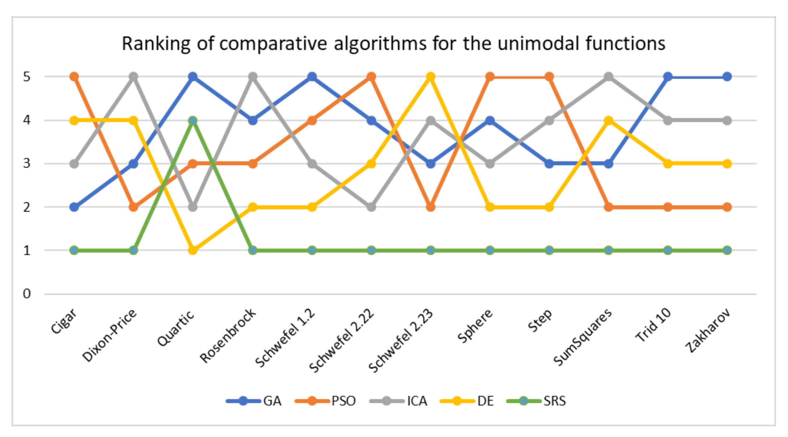
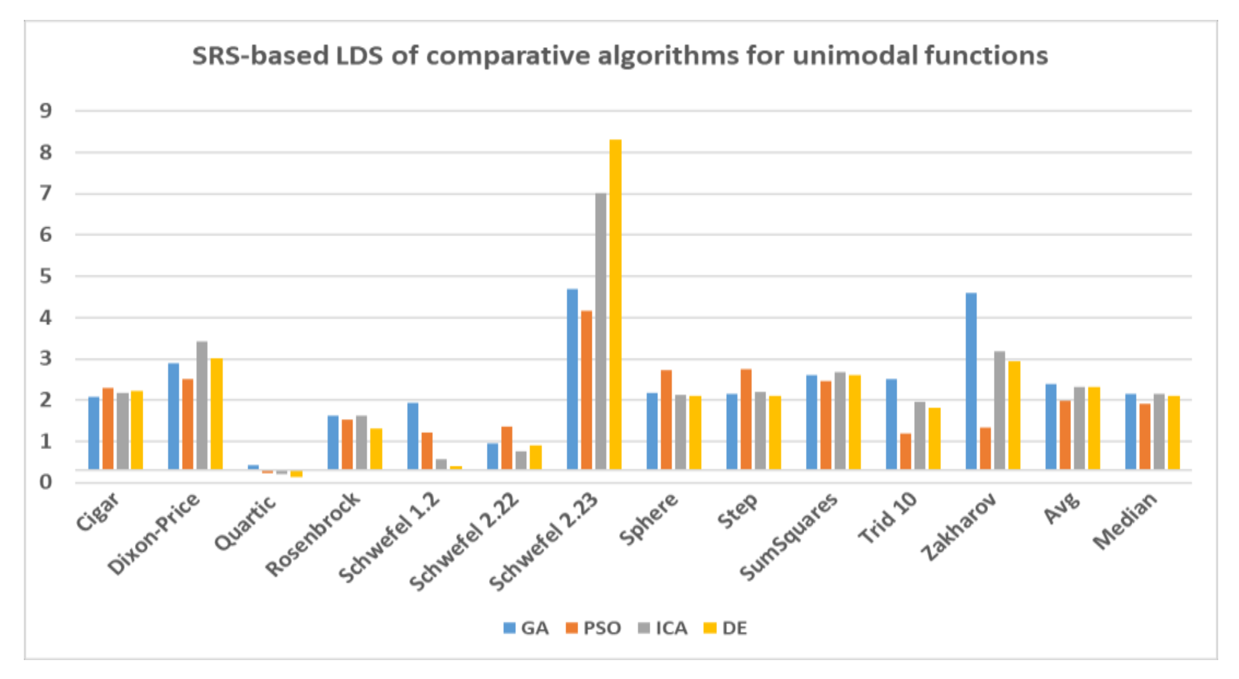
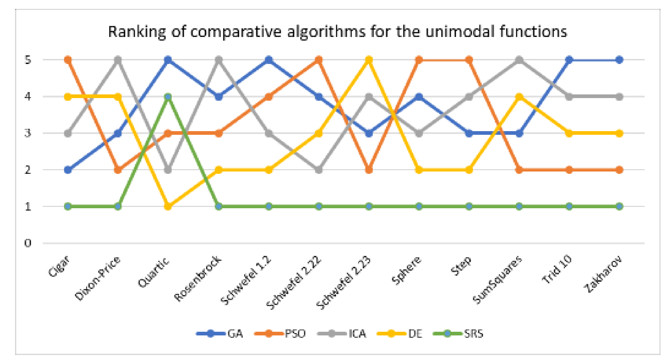
In this paper, a high-performance combinatorial search algorithm called SRS is introduced. SRS was inspired by the plant root growth in soil that occurs to find higher densities of nutrition and water. By mapping solutions to the root and then utilizing three different types of roots with different search characteristics, the algorithm shows high efficiency in both exploration and exploitation activities. Mature roots are responsible for exploration, while immature roots help the SRS escape from local optima traps and non-promising points. Meanwhile, hair roots as very short life searching elements try to search around the best-found solutions for finding higher satisfying points. To evaluate the performance of the SRS and compare its efficiency with those of other algorithms, a complete experimental test was conducted. Twenty-four unimodal and multimodal test functions were employed, and GA, PSO, ICA and DE were applied as comparative algorithms for SRS to find the optimal values of the test functions. To ensure that the collected results were reliable and accurate, every algorithm was executed 40 times per test function, and the average of the results was used in the comparisons.

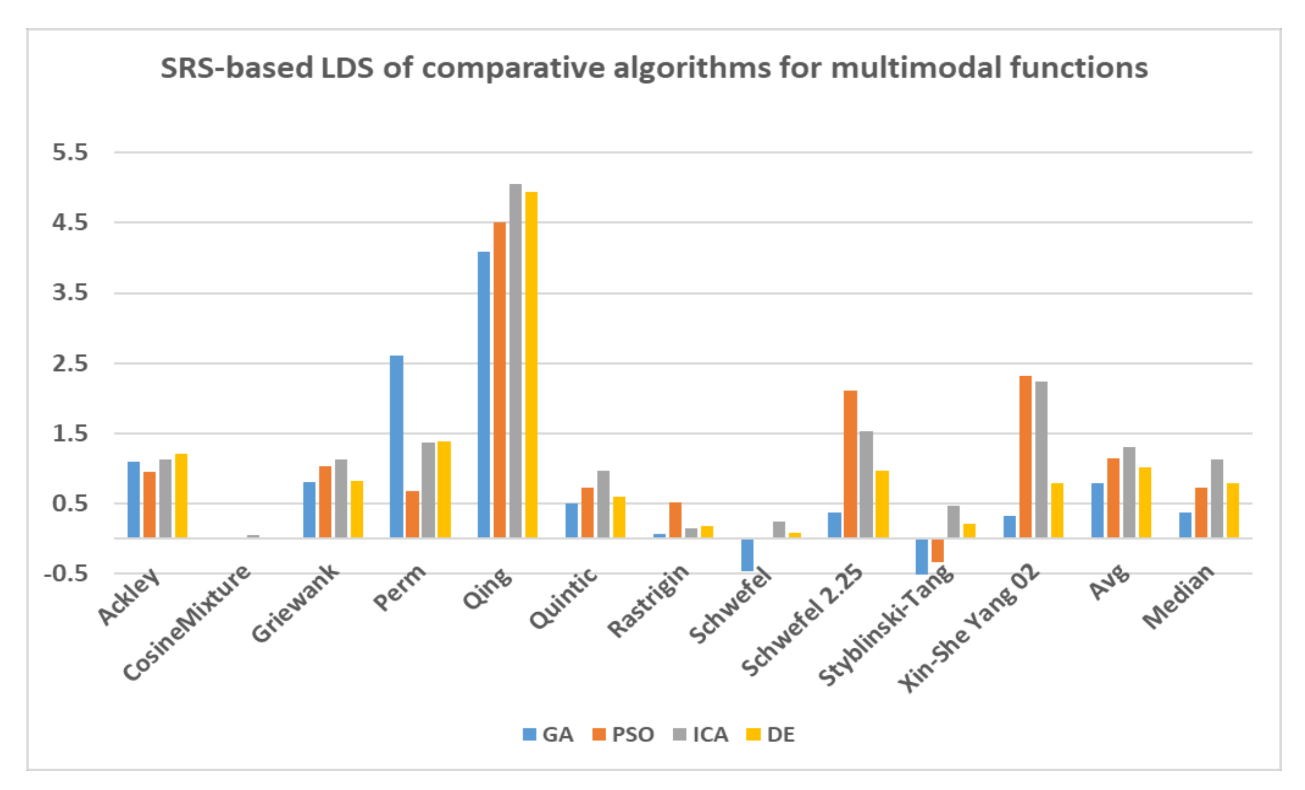
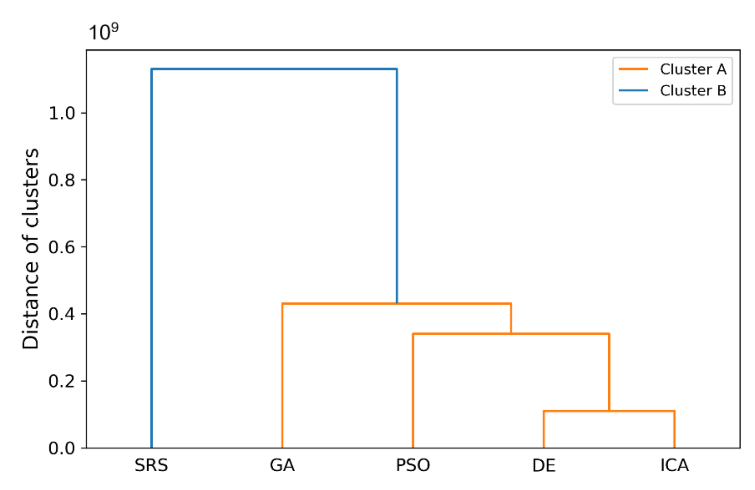
In investigating unimodal test functions, the collected results demonstrated that the SRS performed significantly better than the comparative algorithms, except for the quartic function. Therefore, the SRS won the competition for 91.67% of the functions. For the multimodal test functions, the achieved results indicated that the SRS prevailed 81.81% of the time. Overall, the aggregated results for the unimodal and multimodal test functions indicated that SRS is superior to the comparative algorithms for 86.96% of the test functions used. The higher efficiency in addressing unimodal and multimodal functions demonstrates that the SRS has strong ability to coordinate exploitation and exploration in a way that local optima points are not able to catch it into the traps. Briefly, based on the experimental results and discussion provided here, it can be concluded that the SRS is a formidable competitor for currently well-known combinatorial search algorithms in solving different types of optimization search problems. Well-defined structures and carefully tuned operators are the strengths of the SRS to solving np-hard optimization problems.

Despite the discussed capabilities of the SRS, there are some aspects of the algorithm that can still be upgraded. In terms of functional settings, the SRS enjoys many parameters to customize the functionality of the algorithm. Different values for these parameters may cause different effects in solving various types of optimization problems. Therefore, in the future, efforts should be focused on finding effective values for these parameters. Furthermore, these parameters exert mutual effects on the performance and final achieved solutions. Additional research is needed to regulate the relations among these parameters to be able to run the algorithm effectively by setting a smaller number of parameters. In addition, SRS must be applied in solving several benchmarks as well as real-world optimization problems to determine its strengths and weaknesses as a further matter, the HRG operation was not utilized in the conducted experimental test to provide a more suitable test environment for examining the core exploration and exploitation behaviors of the mature and immature roots. In the future, the performance of the SRS will be achieved by applying a well-organized HRG when solving np-hard problems.

References

1. Holland, J.H. Adaptation in Natural and Artificial Systems: An Introductory Analysis with Applications to Biology, Control, and Artificial Intelligence; University of Michigan Press: Ann Arbor, MI, USA, 1975. [Google Scholar]
2. Kennedy, J.; Eberhart, R. Particle swarm optimization. In Proceedings of the ICNN’95—International Conference on Neural Networks, Perth, WA, Australia, 27 November–1 December 1995; Volume 1944, pp. 1942–1948. [Google Scholar]
3. Ma, Z.Y.; Yuan, X.; Han, S.; Sun, D.; Ma, Y. Improved Chaotic Particle Swarm Optimization Algorithm with More Symmetric Distribution for Numerical Function Optimization. Symmetry 2019, 11, 876. [Google Scholar] [CrossRef] [Green Version]
4. Dorigo, M. Optimization, Learning and Natural Algorithms. Ph.D. Thesis, Politecnico di Milano, Milan, Italy, 1992. [Google Scholar]
5. Zhao, H.G.; Gao, W.; Deng, W.; Sun, M. Study on an Adaptive Co-Evolutionary ACO Algorithm for Complex Optimization Problems. Symmetry 2018, 10, 104. [Google Scholar] [CrossRef] [Green Version]
6. Li, X.L.; Shao, Z.J.; Qian, J.X. An optimizing method based on autonomous animals: Fish-swarm algorithm. Syst. Eng. Theory Pract. 2002, 22, 32–38. [Google Scholar]
7. Farmer, J.D.; Packard, N.H.; Perelson, A.S. The immune system, adaptation, and machine learning. Phys. D 1986, 2, 187–204. [Google Scholar] [CrossRef]
8. Passino, K.M. Biomimicry of bacterial foraging for distributed optimization and control. IEEE Control Syst. 2002, 22, 52–67. [Google Scholar]
9. Chen, Y.-P.; Li, Y.; Wang, G.; Zheng, Y.-F.; Xu, Q.; Fan, J.-H.; Cui, X.-T. A novel bacterial foraging optimization algorithm for feature selection. Expert Syst. Appl. 2017, 83, 1–17. [Google Scholar] [CrossRef]
10. Yang, X.-S. A New Metaheuristic Bat-Inspired Algorithm. In Nature Inspired Cooperative Strategies for Optimization, Studies in Computational Intelligence; Springer: Berlin/Heidelberg, Germany, 2010; Volume 284, pp. 65–74. [Google Scholar]
11. Meng, X.-B.; Gao, X.Z.; Liu, Y.; Zhang, H. A novel bat algorithm with habitat selection and Doppler effect in echoes for optimization. Expert Syst. Appl. 2015, 42, 6350–6364. [Google Scholar] [CrossRef]
12. Atashpaz-Gargari, E.; Lucas, C. Imperialist competitive algorithm: An algorithm for optimization inspired by imperialistic competition. In Proceedings of the 2007 IEEE Congress on Evolutionary Computation, Singapore, 25–28 September 2007; pp. 4661–4667. [Google Scholar]
13. Jula, A.; Othman, Z.; Sundararajan, E. Imperialist competitive algorithm with PROCLUS classifier for service time optimization in cloud computing service composition. Expert Syst. Appl. 2015, 42, 135–145. [Google Scholar] [CrossRef]
14. Jula, A.; Naseri, N.K.; Rahmani, A.M. Gravitational Attraction Search with Virtual Mass (GASVM) to solve Static Grid Job scheduling Problem. J. Math. Comput. Sci. 2010, 1, 305–312. [Google Scholar] [CrossRef]
15. Webster, B.; Bernhard, P.J. A Local Search Optimization Algorithm Based on Natural Principles of Gravitation. In Proceedings of the International Conference on Information and Knowledge Engineering, Las Vegas, NV, USA, 23–26 June 2003; pp. 255–261. [Google Scholar]
16. Lee, Z.-J.; Su, S.-F.; Chuang, C.-C.; Liu, K.-H. Genetic algorithm with ant colony optimization (GA-ACO) for multiple sequence alignment. Appl. Soft Comput. 2008, 8, 55–78. [Google Scholar] [CrossRef]
17. Ying, S.; Zengqiang, C.; Zhuzhi, Y. New Chaotic PSO-Based Neural Network Predictive Control for Nonlinear Process. Neural Netw. IEEE Trans. 2007, 18, 595–601. [Google Scholar] [CrossRef]
18. Zhang, Z.; Zhang, N.; Feng, Z. Multi-satellite control resource scheduling based on ant colony optimization. Expert Syst. Appl. 2014, 41, 2816–2823. [Google Scholar] [CrossRef]
19. Moscato, P. Memetic algorithms: A short introduction. In New Ideas in Optimization; David, C., Marco, D., Fred, G., Dipankar, D., Pablo, M., Riccardo, P., Kenneth, V.P., Eds.; McGraw-Hill Ltd.: Maidenhead, UK, 1999; pp. 219–234. [Google Scholar]
20. Yong, W.; Lin, L. Heterogeneous Redundancy Allocation for Series-Parallel Multi-State Systems Using Hybrid Particle Swarm Optimization and Local Search. Syst. Man Cybern. Part A Syst. Hum. Ieee Trans. 2012, 42, 464–474. [Google Scholar] [CrossRef]
21. Yang, P.; Yang, H.; Qiu, W.; Wang, S.; Li, C. Optimal approach on net routing for VLSI physical design based on Tabu-ant colonies modeling. Appl. Soft Comput. 2014, 21, 376–381. [Google Scholar] [CrossRef]
22. Jula, A.; Othman, Z.; Sundararajan, E. A Hybrid Imperialist Competitive-Gravitational Attraction Search Algorithm to Optimize Cloud Service Composition. In Proceedings of the 2013 IEEE Workshop on Memetic Computing (MC), Singapore, 16–19 April 2013; pp. 37–43. [Google Scholar]
23. Jula, A.; Naseri, N.K. A Hybrid Genetic Algorithm-Gravitational Attraction Search algorithm (HYGAGA) to Solve Grid Task Scheduling Problem. In Proceedings of the International Conference on Soft Computing and its Applications(ICSCA’2012), San Francisco, CA, USA, 24–26 October 2012; pp. 158–162. [Google Scholar]
24. Amato, F.; Castiglione, A.; Moscato, V.; Picariello, A.; Sperlì, G. Multimedia summarization using social media content. Multimed. Tools Appl. 2018, 77, 17803–17827. [Google Scholar] [CrossRef]
25. Zhu, X.; Wang, N. Cuckoo search algorithm with onlooker bee search for modeling PEMFCs using T2FNN. Eng. Appl. Artif. Intell. 2019, 85, 740–753. [Google Scholar] [CrossRef]
26. Garz, P.C.; Keijzer, F. Plants: Adaptive behavior, root-brains, and minimal cognition. Adapt. Behav. Anim. Animat. Softw. Agents Robot. Adapt. Syst. 2011, 19, 155–171. [Google Scholar] [CrossRef]
27. Zhang, H.; Zhu, Y.; Chen, H. Root Growth Model for Simulation of Plant Root System and Numerical Function Optimization. In Intelligent Computing Technology; Huang, D.-S., Jiang, C., Bevilacqua, V., Figueroa, J., Eds.; Springer: Berlin/Heidelberg, Germany, 2012; Volume 7389, pp. 641–648. [Google Scholar]
28. Qi, X.; Zhu, Y.; Chen, H.; Zhang, D.; Niu, B. An Idea Based on Plant Root Growth for Numerical Optimization. In Intelligent Computing Theories and Technology; Huang, D.-S., Jo, K.-H., Zhou, Y.-Q., Han, K., Eds.; Springer: Berlin/Heidelberg, Germany, 2013; Volume 7996, pp. 571–578. [Google Scholar]
29. Ma, L.; Hu, K.; Zhu, Y.; Chen, H.; He, M. A Novel Plant Root Foraging Algorithm for Image Segmentation Problems. Math. Probl. Eng. 2014, 2014, 16. [Google Scholar] [CrossRef]
30. Ma, L.; Zhu, Y.; Liu, Y.; Tian, L.; Chen, H. A novel bionic algorithm inspired by plant root foraging behaviors. Appl. Soft. Comput. 2015, 37, 95–113. [Google Scholar] [CrossRef]
31. Qi, X.; Zhu, Y.; Zhang, H.; Zhang, D.; Wu, J. A novel bio-inspired algorithm based on plant root growth model for data clustering. In Proceedings of the 35th Control Conference (CCC), Chengdu, China, 27–29 July 2016; pp. 9183–9188. [Google Scholar]
32. Naseri, N.K.; Sundararajan, E.; Ayob, M.; Jula, A. Smart Root Search (SRS): A New Search Algorithm to Investigate Combinatorial Problems. In Proceedings of the 2015 Seventh International Conference on Computational Intelligence, Modelling and Simulation (CIMSim), Kuantan, Malaysia, 27–29 July 2015; pp. 1–16. [Google Scholar]
33. Hill, P.S. Vibrational Communication in Animals; Harvard University Press: Cambridge, MA, USA, 2008. [Google Scholar]
34. Buhner, S.H. Plant Intelligence and the Imaginal Realm beyond the Doors of Perception into the Dreaming of Earth; Inner Traditions Bear and Company: Rochester, VT, USA, 2014; p. 576. [Google Scholar]
35. Jung, J.K.H.; McCouch, S.R. Getting to the roots of it: Genetic and hormonal control of root architecture. Front. Plant Sci. 2013, 4. [Google Scholar] [CrossRef] [Green Version]
36. Takahashi, N.; Yamazaki, Y.; Kobayashi, A.; Higashitani, A.; Takahashi, H. Hydrotropism Interacts with Gravitropism by Degrading Amyloplasts in Seedling Roots of Arabidopsis and Radish. Plant Physiol. 2003, 132, 805–810. [Google Scholar] [CrossRef] [Green Version]
37. Moriwaki, T.; Miyazawa, Y.; Kobayashi, A.; Takahashi, H. Molecular mechanisms of hydrotropism in seedling roots of Arabidopsis thaliana (Brassicaceae). Am. J. Bot. 2013, 100, 25–34. [Google Scholar] [CrossRef]
38. Prieto, I.; Armas, C.; Pugnaire, F.I. Hydraulic lift promotes selective root foraging in nutrient-rich soil patches. Funct. Plant Biol. 2012, 39, 804–812. [Google Scholar] [CrossRef] [Green Version]
39. Hultine, K.R.; Cable, W.L.; Burgess, S.S.; Williams, D.G. Hydraulic redistribution by deep roots of a Chihuahuan Desert phreatophyte. Tree Physiol. 2003, 23, 353–360. [Google Scholar] [CrossRef] [Green Version]
40. Blum, A. Plant Water Relations, Plant Stress and Plant Production. In Plant Breeding for Water-Limited Environments; Springer: New York, NY, USA, 2011; pp. 11–52. [Google Scholar] [CrossRef]
41. López-Bucio, J.; Cruz-Ramírez, A.; Herrera-Estrella, L. The role of nutrient availability in regulating root architecture. Curr. Opin. Plant Biol. 2003, 6, 280–287. [Google Scholar] [CrossRef]
42. Signora, L.; De Smet, I.; Foyer, C.H.; Zhang, H. ABA plays a central role in mediating the regulatory effects of nitrate on root branching in Arabidopsis. Plant J. 2001, 28, 655–662. [Google Scholar] [CrossRef] [Green Version]
43. Tian, Q.; Chen, F.; Zhang, F.; Mi, G. Possible Involvement of Cytokinin in Nitrate-mediated Root Growth in Maize. Plant Soil 2005, 277, 185–196. [Google Scholar] [CrossRef]
44. Linkohr, B.I.; Williamson, L.C.; Fitter, A.H.; Leyser, H.M.O. Nitrate and phosphate availability and distribution have different effects on root system architecture of Arabidopsis. Plant J. 2002, 29, 751–760. [Google Scholar] [CrossRef] [Green Version]
45. Jiang, C.; Gao, X.; Liao, L.; Harberd, N.P.; Fu, X. Phosphate Starvation Root Architecture and Anthocyanin Accumulation Responses Are Modulated by the Gibberellin-DELLA Signaling Pathway in Arabidopsis. Plant Physiol. 2007, 145, 1460–1470. [Google Scholar] [CrossRef] [Green Version]
46. Bates, T.R.; Lynch, J.P. Plant growth and phosphorus accumulation of wild type and two root hair mutants of Arabidopsis thaliana (Brassicaceae). Am. J. Bot. 2000, 87, 958–963. [Google Scholar] [CrossRef] [Green Version]
47. Bruce, T.J.A.; Matthes, M.C.; Napier, J.A.; Pickett, J.A. Stressful “memories” of plants: Evidence and possible mechanisms. Plant Sci. 2007, 173, 603–608. [Google Scholar] [CrossRef]
48. Walter, J.; Nagy, L.; Hein, R.; Rascher, U.; Beierkuhnlein, C.; Willner, E.; Jentsch, A. Do plants remember drought? Hints towards a drought-memory in grasses. Environ. Exp. Bot. 2011, 71, 34–40. [Google Scholar] [CrossRef]
49. Fromm, J.; Fei, H. Electrical signaling and gas exchange in maize plants of drying soil. Plant Sci. 1998, 132, 203–213. [Google Scholar] [CrossRef]
50. Mishra, N.S.; Mallick, B.N.; Sopory, S.K. Electrical signal from root to shoot in Sorghum bicolor: Induction of leaf opening and evidence for fast extracellular propagation. Plant Sci. 2001, 160, 237–245. [Google Scholar] [CrossRef]
51. Zhang, H.; Zhu, Y.; Chen, H. Root growth model: A novel approach to numerical function optimization and simulation of plant root system. Soft Comput. 2014, 18, 521–537. [Google Scholar] [CrossRef]
52. Geem, Z.W.; Kim, J.H.; Loganathan, G. A new heuristic optimization algorithm: Harmony search. Simulation 2001, 76, 60–68. [Google Scholar] [CrossRef]
53. Neapolitan, R.; Naimipour, K. Foundations of Algorithms; Jones & Bartlett Learning, LLC: Sudbury, MA, USA, 2010. [Google Scholar]
54. Rubio, V.; Bustos, R.; Irigoyen, M.L.; Cardona-López, X.; Rojas-Triana, M.; Paz-Ares, J. Plant hormones and nutrient signaling. Plant Mol. Biol. 2009, 69, 361–373. [Google Scholar] [CrossRef]
55. López-Bucio, J.; Hernández-Abreu, E.; Sánchez-Calderón, L.; Nieto-Jacobo, M.F.; Simpson, J.; Herrera-Estrella, L. Phosphate Availability Alters Architecture and Causes Changes in Hormone Sensitivity in the Arabidopsis Root System. Plant Physiol. 2002, 129, 244–256. [Google Scholar] [CrossRef] [Green Version]
56. Nacry, P.; Canivenc, G.; Muller, B.; Azmi, A.; Van Onckelen, H.; Rossignol, M.; Doumas, P. A Role for Auxin Redistribution in the Responses of the Root System Architecture to Phosphate Starvation in Arabidopsis. Plant Physiol. 2005, 138, 2061–2074. [Google Scholar] [CrossRef] [Green Version]
57. Beckett, M.; Garnett, S.; Hay, M.; Makings, E.; Marriott, H.; Nieuwenhuizen, N.; Sabela, G.; Scheffler, C.; Steenkamp, L.; Viljoen, K.; et al. Siyavula: Life Sciences Grade 10; Siyavula, Ed.; Connexions Rice University: Houston, TX, USA, 2011. [Google Scholar]
58. Vafaee, F.; Turan, G.; Nelson, P.C.; Berger-Wolf, T.Y. Balancing the Exploration and Exploitation in an Adaptive Diversity Guided Genetic Algorithm. In Proceedings of the 2014 IEEE Congress on Evolutionary Computation (CEC), Beijing, China, 6–11 July 2014; pp. 2570–2577. [Google Scholar]
59. Chen, J.; Xin, B.; Peng, Z.H.; Dou, L.H.; Zhang, J.A. Optimal Contraction Theorem for Exploration-Exploitation Tradeoff in Search and Optimization. IEEE Trans. Syst. Man Cybern. Part A Syst. Hum. 2009, 39, 680–691. [Google Scholar] [CrossRef]
60. Lipowski, A.; Lipowska, D. Roulette-wheel selection via stochastic acceptance. Phys. A Stat. Mech. Its Appl. 2012, 391, 2193–2196. [Google Scholar] [CrossRef] [Green Version]
61. Rudolph, G. Convergence Properties of Evolutionary Algorithms; Verlag Dr. Kovac: Hamburg, Germany, 1997. [Google Scholar]
62. He, J.; Lin, G.M. Average Convergence Rate of Evolutionary Algorithms. IEEE Trans. Evol. Comput. 2016, 20, 316–321. [Google Scholar] [CrossRef] [Green Version]
63. Karaboga, D.; Basturk, B. A powerful and efficient algorithm for numerical function optimization: Artificial bee colony (ABC) algorithm. J. Glob. Optim. 2007, 39, 459–471. [Google Scholar] [CrossRef]
64. Homaifar, A.; Qi, C.X.; Lai, S.H. Constrained optimization via genetic algorithms. Simulation 1994, 62, 242–253. [Google Scholar] [CrossRef]
65. Kennedy, J.; Kennedy, J.F.; Eberhart, R.C.; Shi, Y. Swarm Intelligence; Morgan Kaufmann: San Francisco, CA, USA, 2001. [Google Scholar]
66. Karaboga, D.; Akay, B. A comparative study of Artificial Bee Colony algorithm. Appl. Math. Comput. 2009, 214, 108–132. [Google Scholar] [CrossRef]
67. Adorio, E.P.; Diliman, U. Mvf-Multivariate Test Functions Library in C for Unconstrained Global Optimization; University of the Philippines Diliman: Quezon City, Philippines, 2005. [Google Scholar]
68. Gavana, A. Test Functions Index. Available online: http://infinity77.net/global_optimization/test_functions.html (accessed on 27 April 2016).
69. Jamil, M.; Yang, X.-S. A literature survey of benchmark functions for global optimisation problems. Int. J. Math. Model. Numer. Optim. 2013, 4, 150–194. [Google Scholar] [CrossRef] [Green Version]
70. Yang, X.S. Appendix A: Test problems in optimization. Eng. Optim. 2010, 1, 261–266. [Google Scholar]
71. Jula, A.; Nilsaz, H.; Sundararajan, E.; Othman, Z. A new dataset and benchmark for cloud computing service composition. In Proceedings of the 2014 5th International Conference on Intelligent Systems, Modelling and Simulation, Langkawi, Malaysia, 27–29 January 2014; pp. 83–86. [Google Scholar]
72. Everitt, B.S. Cluster analysis of subjects, hierarchical methods. Encycl. Biostat. 2005, 2. [Google Scholar] [CrossRef]
73. Day, W.H.E.; Edelsbrunner, H. Efficient algorithms for agglomerative hierarchical clustering methods. J. Classif. 1984, 1, 7–24. [Google Scholar] [CrossRef]
74. CaliŃski, T. Dendrogram. Wiley Statsref Stat. Ref. Online 2014. [Google Scholar] [CrossRef]
75. Wells, C.S. Encyclopedia of Research Design. In Encyclopedia of Research Design; Salkind, N.J., Ed.; SAGE Publications, Inc.: Thousand Oaks, CA, USA, 2010. [Google Scholar] [CrossRef]
76. Kim, H.-Y. Analysis of variance (ANOVA) comparing means of more than two groups. Restor. Dent. Endod. 2014, 39, 74–77. [Google Scholar] [CrossRef] [PubMed] [Green Version]
77. McHugh, M.L. The Chi-square test of independence. Biochem. Med. 2013, 23, 143–149. [Google Scholar] [CrossRef] [PubMed] [Green Version]
Figure 1. The smart root search (SRS) flowchart.
Symmetry 12 02025 g001
Figure 2. The basic structure of an SRS root. The first row represents the structure while the second row explains what should be assigned to every element of the structure.
Symmetry 12 02025 g002
Figure 3. Types of roots [57].
Symmetry 12 02025 g003
Figure 4. An example of NC-based grouping affects parent root branching when locating in a (a) promising part of search space, and (b) unpromising part of search space.
Symmetry 12 02025 g004
Figure 5. Changes in moisture percentage (MP) value of roots over puberty.
Symmetry 12 02025 g005
Figure 6. Pseudo code for SRS algorithm.
Symmetry 12 02025 g006
Figure 7. Converges of SRS toward global optima; (a) shows how search space gets divided into four subspaces; (b) shows process of generating random solutions in subspaces and choosing optimal solution of each of them; (c) demonstrates how number of solutions gets less in subspaces that could not find proper solutions while it gets more in promising subspaces; (d,e) represent the worst subspaces having no solution contrasted with the best subspace determined gradually; (f) SRS found the global optima in the best subspace.
Symmetry 12 02025 g007
Figure 8. How SRS outperforms the other algorithms in benchmarking unimodal test function.
Symmetry 12 02025 g008
Figure 9. LDS of the comparative algorithms for unimodal functions based on SRS.
Symmetry 12 02025 g009
Figure 10. How SRS outperforms the other algorithms in benchmarking multimodal test function.
Symmetry 12 02025 g010
Figure 11. LDS of the comparative algorithms for unimodal functions based on SRS.
Symmetry 12 02025 g011
Figure 12. Dendrogram diagram plotted using Agglomerative hierarchical clustering results of comparative algorithms.
Symmetry 12 02025 g012