General Response Formula for CFD Pseudo-Fractional 2D Continuous Linear Systems Described by the Roesser Model

Abstract

In many engineering problems associated with various physical phenomena, there occurs a necessity of analysis of signals that are described by multidimensional functions of more than one variable such as time t or space coordinates x, y, z. Therefore, in such cases, we should consider dynamical models of two or more dimensions. In this paper, a new two-dimensional (2D) model described by the Roesser type of state-space equations will be considered. In the introduced model, partial differential operators described by the Conformable Fractional Derivative (CFD) definition with respect to the first (horizontal) and second (vertical) variables will be applied. For the model under consideration, the general response formula is derived using the inverse fractional Laplace method. Next, the properties of the solution will be considered. Usefulness of the general response formula will be discussed and illustrated by a numerical example.

1. Introduction

In the analysis of many real-world problems that arise in modern engineering, considerations cannot be limited to only one dimension, predominately the time variable. The researchers should consider these issues in a broader aspect, in more than one dimension, i.e., time and some spatial variables. Therefore, for the last few decades in control theory, we observe a growing interest of multidimensional dynamic systems. The state-of-the-art in this class of dynamic systems, their properties and control methods are presented in the monographs [1,2,3].

In control theory two-dimensional systems (2D systems) are most often modelled by 2D state-space differential or difference equations. For discrete two-dimensional (2D) systems, the most popular are the structures of the state-space models proposed by Roesser [4], Fornasini and Marchesini [5,6], and Kurek [7]. These models are also adopted for continuous domain in [8,9,10,11].

Recently, in the analysis of many physical phenomena, researchers consider partial differential equations in two dimensions using fractional (non-integer) order partial differential operators. The most interesting areas where this approach has found application are two-dimensional models describing the dynamics of dislocation of atoms in crystals [12], processes of anomalous diffusion [13,14,15,16], nonlinear cable equations used in electrophysiology [17] or in investigating of problems connected with thermoelasticity [18]. The non-integer order of derivation introduces an additional degree of freedom to the model. Therefore, its accuracy is much better in comparison with the classical integer-order models of different phenomena.

There are many different definitions of non-integer (fractional) order derivatives such as Riemann–Liouville, Grünwald–Letnikov or Caputo fractional derivatives [19,20,21,22].

The symmetry properties of fractional differential equations have been considered by many researchers. Gazizov et al. investigated Lie point symmetries of nonlinear anomalous diffusion equations with time-domain Riemann–Liouville and Caputo fractional derivatives in [23]. The obtained symmetries are applied for constructing exact solutions of the equations. In [24], the radial symmetry of standing waves for a nonlinear Schrödinger equation involving the fractional Laplacian and Hardy potential has been investigated. An application of Lie groups to solve the space-time fractional Burgers’ equation has been presented in [25], where the authors have shown that the Lie symmetry method may be used to reduce the partial fractional-order differential equations to the system described by ordinary differential equations. Therefore, the Lie group method is one of the most effective techniques to find exact solutions of partial differential equations. The processes considered in the above papers may be described by the model that will be introduced in this article.

In the last few years, many new well-behaved fractional and pseudo-fractional derivatives definitions appeared. The Conformable Fractional Derivative (CFD) was introduced by Khalil et al. in [26], and in [27] it was shown that this new definition has similar properties as classical (integer) order derivatives including the chain rule, integration by parts, Taylor power series expansion and Laplace transforms. A generalisation of the CFD operator and its physical interpretation has been presented in [28].

In this paper, a new two-dimensional continuous non-integer order Roesser-type model with partial derivatives described by the Conformable Fractional Derivative definition will be introduced. Next, the 2D inverse fractional Laplace transform method will be used to derive the general response formula for the system. It will be shown that the classical Cayley–Hamilton theorem can be extended for such a new class of 2D fractional order systems. Finally, a numerical example will be presented, where the step response of the system will be investigated.

Similar considerations were conducted for Roesser and Fornasini–Marchesini structures of 2D fractional order systems in [29,30], where a Caputo-type fractional differential operator was used. A non-integer order CFD derivative is more comfortable in theoretical analysis and more efficient in numerical computations; therefore, it may be useful in the modelling of multidimensional problems in control theory.

To the best knowledge of the author, the two-dimensional continuous CFD pseudo-fractional systems described by the Roesser model have not been considered yet.

2. Conformable Fractional Derivative Definition and Its Properties

In this section, we will present a basic definition of CFD non-integer order derivative in one and two dimensions and briefly recall some properties of this mathematical differential operator. Next, we will show that the modified (fractional) Laplace transform is very useful in further consideration of the models consisting CFD derivatives.

Let ${\mathbb{R}}^{n\times m}$ be the set of $n\times m$ real matrices, the $n\times n$ identity matrix will be denoted by ${\mathbb{I}}_n$ and $n\times n$ matrix with all zero elements by $0_n$.

Definition 1

([26]). The Conformable Fractional Derivative (CFD) of a real continuous-time function $f\left(t\right)$, $t\in [0,\infty )$ of order $\alpha \in (0,1)$ is defined by

$$D^{\alpha }f\left(t\right)=\underset{ϵ\to 0}{lim}\frac{f(t+ϵt^{1-\alpha })-f\left(t\right)}{ϵ},$$

(1)

where $D^{\alpha }f\left(0\right)={lim}_{t\to 0^{+}}{D}^{\alpha }f\left(t\right)$.

We say that the function $f\left(t\right)$ is $\alpha$-differentiable if there exists the CFD derivative $D^{\alpha }f\left(t\right)$. It is also well-known [26,27] that if the function $f\left(t\right)$ is differentiable, then

$$D^{\alpha }f\left(t\right)=t^{1-\alpha }\frac{\mathrm{d}}{\mathrm{d}t}f\left(t\right).$$

(2)

The properties of the mathematical operator CFD were investigated in [27] and its physical interpretation was discussed in [28]. Moreover, it was shown there that the modified type of Laplace transform may be useful for the analysis of analytical problems related to CFD derivatives.

Definition 2

([27]). Let $0<\alpha \le 1$ and $f:[0,\infty )\to \mathbb{R}$, then the fractional one-sided Laplace transform of α-order of $f\left(t\right)$ is defined by

$${\mathcal{L}}^{\alpha }\left\{f\left(t\right)\right\}=F^{\alpha }\left(s\right)=\underset{0}{\overset{\infty }{\int }}{e}^{-s\frac{t^{\alpha }}{\alpha }}f\left(t\right)t^{\alpha -1}\mathrm{d}t.$$

(3)

In [27], it has been shown that the fractional Laplace transform is a special case of the classical Laplace transform, where the time variable is replaced by a modified variable ${\left(\alpha t\right)}^{1/\alpha }$ as follows from the following lemma.

Lemma 1

([27]). Let $F^{\alpha }\left(s\right)$ be the one-sided fractional Laplace transform of a function $f\left(t\right)$. Then,

$$F^{\alpha }\left(s\right)=\mathcal{L}\left\{f\left[{\left(\alpha t\right)}^{1/\alpha }\right]\right\},$$

(4)

where

$$\mathcal{L}\left\{f\left(t\right)\right\}=F\left(s\right)=\underset{0}{\overset{\infty }{\int }}{e}^{-st}f\left(t\right)\mathrm{d}t$$

(5)

is the standard one-sided Laplace transform.

The greatest benefit of the fractional Laplace transform application for non-integer differential equations solving is that the modified transform of a CFD operator is similar to the Laplace transform of integer order derivative. Therefore, the analysis of CFD differential equations may be considered using well-known methods from the classical integer order calculus, but one should remember that the complex variable s in the fractional Laplace transform and s in the classical Laplace transform are not isomorphic.

Theorem 1

([27]). The fractional Laplace transform (3) of the Conformable Fractional Derivative operator (1) is given by

$${\mathcal{L}}^{\alpha }\left\{D^{\alpha }f\left(t\right)\right\}=s{F}^{\alpha }\left(s\right)-f\left(0^{+}\right),$$

(6)

where $\alpha \in \mathbb{R}$ is the non-integer order of CFD derivative.

Next, we will derive the convolution formula for the fractional Laplace transform. It is well known that for the classical Laplace transform of two continuous-time functions $f\left(t\right)$ and $g\left(t\right)$, we have the following convolution formula,

$$\begin{array}{cc}\hfill F\left(s\right)G\left(s\right)=& \mathcal{L}\left\{f\left(t\right)\ast g\left(t\right)\right\}\hfill \\ \hfill =& \mathcal{L}\left\{\underset{0}{\overset{t}{\int }}f(t-\tau )g\left(\tau \right)\mathrm{d}\tau \right\}.\hfill \end{array}$$

(7)

Now, let us define the modified convolution integral called $\alpha$-convolution integral.

Definition 3

([31]). Let $f\left(t\right)$ and $g\left(t\right)$ be two continuous-time functions. We define the α-convolution of $f\left(t\right)$ and $g\left(t\right)$ by

$$f\left(t\right){\ast }_{\alpha }g\left(t\right)=\underset{0}{\overset{t}{\int }}f\left({\left(t^{\alpha }-{\tau }^{\alpha }\right)}^{\frac{1}{\alpha }}\right)g\left(\tau \right)\frac{\mathrm{d}\tau }{{\tau }^{1-\alpha }},$$

(8)

where $\alpha >0$ is an arbitrary non-integer order of the convolution.

The commutativity of the $\alpha$-convolution of two functions is satisfied, as [31]

$$f\left(t\right){\ast }_{\alpha }g\left(t\right)=g\left(t\right){\ast }_{\alpha }f\left(t\right).$$

(9)

Finally, we extend the convolution Formula (7) for the fractional Laplace transform.

Theorem 2

([31]). Fractional Laplace transform of the α-convolution of functions $f\left(t\right)$ and $g\left(t\right)$, where $\alpha >0$ is the order of the transform, is given by

$${\mathcal{L}}_{\alpha }\left\{f\left(t\right){\ast }_{\alpha }g\left(t\right)\right\}=F_{\alpha }\left(s\right)G_{\alpha }\left(s\right).$$

(10)

In this paper, we will investigate a dynamic system that is described in two dimensions (containing two independent variables), therefore using Definition 1 we will introduce the following definition of CFD non-integer order partial derivative of a 2D continuous function $f(t_1,t_2)$ of two independent variables $t_1\ge 0$ and $t_2\ge 0$.

Definition 4.

The $\alpha \in (0,1)$ order partial CFD derivative of a 2D continuous function $f(t_1,t_2)$ with respect to the variable $t_1$ is defined by the formula

$$D_{t_1}^{\alpha }f(t_1,t_2)=\frac{{\partial }^{\alpha }}{\partial {t_1}^{\alpha }}f(t_1,t_2)=\underset{ϵ\to 0}{lim}\frac{f(t_1+ϵ{t_1}^{1-\alpha },t_2)-f(t_1,t_2)}{ϵ},$$

(11)

In a similar way, we define the non-integer order partial CFD derivative of a function $f(t_1,t_2)$ with respect to the second variable $t_2$.

3. The CFD Pseudo-Fractional 2D System Described by the Roesser Model

Now let us consider the CFD pseudo-fractional 2D continuous system described by the state equations

$$\left[\begin{array}{c}{D}_{t_1}^{\alpha }{x}^h(t_1,t_2)\\ D_{t_2}^{\beta }{x}^v(t_1,t_2)\end{array}\right]=\left[\begin{array}{cc}{A}_{11}& A_{12}\\ A_{21}& A_{22}\end{array}\right]\left[\begin{array}{c}{x}^h(t_1,t_2)\\ x^v(t_1,t_2)\end{array}\right]+\left[\begin{array}{c}{B}_1\\ B_2\end{array}\right]u(t_1,t_2),$$

(12a)

$$y(t_1,t_2)=C\left[\begin{array}{c}{x}^h(t_1,t_2)\\ x^v(t_1,t_2)\end{array}\right]+Du(t_1,t_2),$$

(12b)

where $x^h(t_1,t_2)\in {\mathbb{R}}^{n_1}$, $x^v(t_1,t_2)\in {\mathbb{R}}^{n_2}$$(n=n_1+n_2)$ are the horizontal and vertical state vectors, respectively; $u(t_1,t_2)\in {\mathbb{R}}^m$ is the input vector; and $y(t_1,t_2)\in {\mathbb{R}}^p$ is the vector of outputs and the matrices $A_{kl}\in {\mathbb{R}}^{n_k\times n_l}$, $B_k\in {\mathbb{R}}^{n_k\times m}$ for $k,l=1,2$; $C\in {\mathbb{R}}^{p\times n}$; $D\in {\mathbb{R}}^{p\times m}$. For each dimension, we have different non-integer orders, $0<\alpha <1$ for horizontal and $0<\beta <1$ for the vertical direction of differentiation.

In the particular case, when we assume $\alpha =1$ and $\beta =1$ in (11), we obtain

$$D_{t_1}^{\alpha }f(t_1,t_2)=\frac{\partial }{\partial t_1}f(t_1,t_2),D_{t_2}^{\alpha }f(t_1,t_2)=\frac{\partial }{\partial t_2}f(t_1,t_2).$$

(13)

and the considered model becomes a continuous counterpart of a discrete integer-order Roesser model described by

$$\left[\begin{array}{c}\frac{\partial }{\partial t_1}{x}^h(t_1,t_2)\\ \frac{\partial }{\partial t_2}{x}^v(t_1,t_2)\end{array}\right]=\left[\begin{array}{cc}{A}_{11}& A_{12}\\ A_{21}& A_{22}\end{array}\right]\left[\begin{array}{c}{x}^h(t_1,t_2)\\ x^v(t_1,t_2)\end{array}\right]+\left[\begin{array}{c}{B}_1\\ B_2\end{array}\right]u(t_1,t_2).$$

(14)

Using any discretisation method, we may express the state Equation (14) in the form of well-known discrete Roesser model [4]. Therefore, the proposed model has a structure similar to the 2D discrete Roesser model introduced in [4] and it is a generalisation of the integer-order model for non-integer orders.

The boundary conditions for (12) are given in the following form,

$$x^h(0,t_2)=h\left(t_2\right)\in {\mathbb{R}}^{n_1}$$

(15a)

and

$$x^v(t_1,0)=v\left(t_1\right)\in {\mathbb{R}}^{n_2}$$

(15b)

for $t_1,t_2\ge 0$, where $h\left(t_2\right)$ and $v\left(t_1\right)$ are assumed boundary continuous real functions.

Note that for the model (12) we assume only Dirichlet-type boundary conditions. This issue is essential in the modelling of phenomena occurring in engineering, where the derivatives of functions at the boundaries of the area of investigation are often difficult to define.

4. General Response Formula

In this section, we will derive a general response formula for the model (12) using the inverse fractional Laplace transform method.

Let $F^{\alpha }(p,t_2)$$\left(F^{\beta }(t_1,s)\right)$ be the fractional $\alpha$-order ($\beta$-order) Laplace transform of a 2D continuous function $f(t_1,t_2)$ with respect to $t_1$ ($t_2$) defined by

$$F^{\alpha }(p,t_2)={\mathcal{L}}_{t_1}^{\alpha }\left\{f(t_1,t_2)\right\}=\underset{0}{\overset{\infty }{\int }}{e}^{-p\frac{t_1^{\alpha }}{\alpha }}f(t_1,t_2)t_1^{\alpha -1}\mathrm{d}{t}_1$$

(16)

and

$$F^{\beta }(t_1,s)={\mathcal{L}}_{t_2}^{\beta }\left\{f(t_1,t_2)\right\}=\underset{0}{\overset{\infty }{\int }}{e}^{-s\frac{t_2^{\beta }}{\beta }}f(t_1,t_2)t_2^{\beta -1}\mathrm{d}{t}_2.$$

(17)

The two-dimensional $(\alpha ,\beta )$-orders fractional Laplace transform of a function $f(t_1,t_2)$ will be denoted by $F^{\alpha \beta }(p,s)$ and defined by

$$\begin{array}{cc}\hfill F^{\alpha \beta }(p,s)& ={\mathcal{L}}_{t_1,t_2}^{\alpha \beta }\left\{f(t_1,t_2)\right\}={\mathcal{L}}_{t_1}^{\alpha }\left\{{\mathcal{L}}_{t_2}^{\beta }\left[f(t_1,t_2)\right]\right\}={\mathcal{L}}_{t_2}^{\beta }\left\{{\mathcal{L}}_{t_1}^{\alpha }\left[f(t_1,t_2)\right]\right\}\hfill \\ \hfill & =\underset{0}{\overset{\infty }{\int }}\underset{0}{\overset{\infty }{\int }}{e}^{-p\frac{t_1^{\alpha }}{\alpha }-s\frac{t_2^{\beta }}{\beta }}f(t_1,t_2)t_1^{\alpha -1}{t}_2^{\beta -1}\mathrm{d}{t}_1\mathrm{d}{t}_2.\hfill \end{array}$$

(18)

Now applying the 2D fractional Laplace transform (18) to both sides of the state Equation (12) and using (6) with respect to both variables $t_1$ and $t_2$ we obtain

$$\begin{array}{cc}\hfill \left[\begin{array}{c}p{X}_{\alpha \beta }^h(p,s)-X_{\beta }^h\left(s\right)\\ s{X}_{\alpha \beta }^v(p,s)-X_{\alpha }^v\left(p\right)\end{array}\right]=& \left[\begin{array}{cc}{A}_{11}& A_{12}\\ A_{21}& A_{22}\end{array}\right]\left[\begin{array}{c}{X}_{\alpha \beta }^h(p,s)\\ X_{\alpha \beta }^v(p,s)\end{array}\right]+\left[\begin{array}{c}{B}_1\\ B_2\end{array}\right]U_{\alpha \beta }(p,s),\hfill \end{array}$$

(19)

where

$$X_{\alpha \beta }^h(p,s)={\mathcal{L}}_{t_1,t_2}^{\alpha \beta }\left\{x^h(t_1,t_2)\right\},$$

$$X_{\alpha \beta }^v(p,s)={\mathcal{L}}_{t_1,t_2}^{\alpha \beta }\left\{x^v(t_1,t_2)\right\}$$

and

$$X_{\beta }^h\left(s\right)=X_{\beta }^h(0,s)={\mathcal{L}}_{t_2}^{\beta }\left\{x^h(0,t_2)\right\}={\mathcal{L}}_{t_2}^{\beta }\left\{h\left(t_2\right)\right\},$$

$$X_{\alpha }^v\left(p\right)=X_{\alpha }^v(p,0)={\mathcal{L}}_{t_1}^{\alpha }\left\{x^v(t_1,0)\right\}={\mathcal{L}}_{t_2}^{\alpha }\left\{v\left(t_1\right)\right\}$$

and $U_{\alpha \beta }(p,s)={\mathcal{L}}_{t_1,t_2}^{\alpha \beta }\left\{u(t_1,t_2)\right\}$, where $\alpha$ ($\beta$) is the order of the fractional Laplace transform with respect to $t_1$ ($t_2$).

Premultiplying (19) by the matrix

$$\mathrm{blockdiag}\left[p^{-1}{\mathbb{I}}_{n_1},s^{-1}{\mathbb{I}}_{n_2}\right]$$

we obtain

$$\begin{array}{cc}\hfill \left[\begin{array}{c}{X}_{\alpha \beta }^h(p,s)\\ X_{\alpha \beta }^v(p,s)\end{array}\right]=& G^{-1}(p,s)\left\{\left[\begin{array}{c}{p}^{-1}{X}_{\beta }^h\left(s\right)\\ s^{-1}{X}_{\alpha }^v\left(p\right)\end{array}\right]+\left[\begin{array}{c}{p}^{-1}{B}_1\\ s^{-1}{B}_2\end{array}\right]U_{\alpha \beta }(p,s)\right\},\hfill \end{array}$$

(20)

where

$$G(p,s)=\left[\begin{array}{cc}{\mathbb{I}}_{n_1}-p^{-1}{A}_{11}& -p^{-1}{A}_{12}\\ -s^{-1}{A}_{21}& {\mathbb{I}}_{n_2}-s^{-1}{A}_{22}\end{array}\right].$$

(21)

Assume that the inverse of the polynomial matrix $G(p,s)$ has the form

$$G^{-1}(p,s)=\sum _{i=0}^{\infty }\sum _{j=0}^{\infty }{T}_{i,j}{p}^{-i}{s}^{-j},$$

(22)

where $T_{i,j}\in {\mathbb{R}}^{n\times n}$ are called the transition matrices.

It is well known that

$$G(p,s)G^{-1}(p,s)=G^{-1}(p,s)G(p,s)={\mathbb{I}}_n.$$

Therefore, using (21) and (22), we obtain

$$\sum _{i=0}^{\infty }\sum _{j=0}^{\infty }\left\{T_{i,j}-T_{1,0}{T}_{i-1,j}-T_{0,1}{T}_{i,j-1}\right\}{p}^{-i}{s}^{-j}={\mathbb{I}}_n,$$

(23)

where

$$T_{1,0}=\left[\begin{array}{cc}{A}_{11}& A_{12}\\ 0& 0\end{array}\right],T_{0,1}=\left[\begin{array}{cc}0& 0\\ A_{21}& A_{22}\end{array}\right].$$

(24)

Comparing the coefficients of both sides of the equality (23) with respect to the corresponding powers of variables p and s, we may formulate the following recursive formula for the computation of transition matrices $T_{ij}$,

$$T_{i,j}=\left\{\begin{array}{cc}{\mathbb{I}}_n\hfill & \mathrm{for}i=j=0,\hfill \\ T_{1,0}{T}_{i-1,j}+T_{0,1}{T}_{i,j-1}\hfill & \mathrm{for}i+j>0(i,j\in {\mathbb{Z}}_{+}),\hfill \\ 0_n\hfill & \mathrm{for}i<0\mathrm{and}/\mathrm{or}j<0.\hfill \end{array}\right.$$

(25)

Substituting the expansion (22) into (20), we obtain

$$\begin{array}{cc}\hfill \left[\begin{array}{c}{X}_{\alpha \beta }^h(p,s)\\ X_{\alpha \beta }^v(p,s)\end{array}\right]=\sum _{i=0}^{\infty }\sum _{j=0}^{\infty }& \left\{T_{i-1,j}\left[\begin{array}{c}{X}_{\beta }^h\left(s\right)\\ 0\end{array}\right]+T_{i,j-1}\left[\begin{array}{c}0\\ X_{\alpha }^v\left(p\right)\end{array}\right]\right.\hfill \\ & \left.+T_{i-1,j}\left[\begin{array}{c}{B}_1\\ 0\end{array}\right]U_{\alpha \beta }(p,s)T_{i,j-1}\left[\begin{array}{c}0\\ B_2\end{array}\right]U_{\alpha \beta }(p,s)\right\}{p}^{-i}{s}^{-j}.\hfill \end{array}$$

(26)

To find an inverse fractional Laplace transform of both sides of (26), we should derive the inverse $\alpha$-order Laplace transform of the expression $s^{-1}$.

First, using Definition 2, we will derive the fractional Laplace transform of a function $t^p$ for $t>0$ and $p>0$ as follows,

$${\mathcal{L}}^{\alpha }\left\{t^p\right\}=\underset{0}{\overset{\infty }{\int }}{e}^{-s\frac{t^{\alpha }}{\alpha }}{t}^{p+\alpha -1}\mathrm{d}t$$

(27)

By the substitution of $x=s\frac{t^{\alpha }}{\alpha }$, we obtain

$$\begin{array}{cc}\hfill {\mathcal{L}}^{\alpha }\left\{t^p\right\}=& \frac{{\alpha }^{\frac{p}{\alpha }}}{s^{1+\frac{p}{\alpha }}}\underset{0}{\overset{\infty }{\int }}{e}^{-x}{x}^{\frac{p}{\alpha }}\mathrm{d}x\hfill \\ \hfill =& \frac{{\alpha }^{\frac{p}{\alpha }}}{s^{1+\frac{p}{\alpha }}}\mathsf{\Gamma }\left(1+\frac{p}{\alpha }\right)\hfill \end{array}$$

(28)

for $p>-\alpha$, as $\mathsf{\Gamma }\left(x\right)=\underset{0}{\overset{\infty }{\int }}{t}^{x-1}{e}^{-t}\mathrm{d}t$, where $x>0$ is called the Euler gamma function.

If we assume that $\gamma =1+\frac{p}{\alpha }$, we may form the expression for the inverse Laplace fractional transform of the operator $\frac{1}{s^{\gamma }}$, where $\gamma >0$ as follows,

$${\mathcal{L}}_{\alpha }^{-1}\left\{\frac{1}{s^{\gamma }}\right\}=\frac{t^{\alpha (\gamma -1)}}{{\alpha }^{\gamma -1}\mathsf{\Gamma }\left(\gamma \right)}.$$

(29)

Applying the inverse fractional Laplace transform with respect to the variables p and s to (26) and taking into account (29) and (10) we obtain

$$\begin{array}{cc}\hfill \left[\begin{array}{c}{x}^h(t_1,t_2)\\ x^v(t_1,t_2)\end{array}\right]=& \left[\begin{array}{cc}{e}^{\frac{A_{11}{t}_1^{\alpha }}{\alpha }}& 0\\ 0& e^{\frac{A_{22}{t}_2^{\beta }}{\beta }}\end{array}\right]\left[\begin{array}{c}h\left(t_2\right)\\ v\left(t_1\right)\end{array}\right]+\sum _{i=0}^{\infty }\sum _{j=0}^{\infty }{T}_{i,j+1}\frac{t_1^{\alpha i}}{{\alpha }^{i}i!}\underset{0}{\overset{t_2}{\int }}\frac{{(t_2^{\beta }-{\tau }_2^{\beta })}^j}{{\beta }^{j}j!{\tau }_2^{1-\beta }}\left[\begin{array}{c}h\left({\tau }_2\right)\\ 0\end{array}\right]\mathrm{d}{\tau }_2\hfill \\ \hfill & +\sum _{i=0}^{\infty }\sum _{j=0}^{\infty }{T}_{i+1,j}\frac{t_2^{\beta j}}{{\beta }^{j}j!}\underset{0}{\overset{t_1}{\int }}\frac{{\left(t_1^{\alpha }-{\tau }_1^{\alpha }\right)}^i}{{\alpha }^{i}i!{\tau }_1^{1-\alpha }}\left[\begin{array}{c}0\\ v\left({\tau }_1\right)\end{array}\right]\mathrm{d}{\tau }_1\hfill \\ \hfill & +\underset{0}{\overset{t_1}{\int }}\left[\begin{array}{c}{e}^{A_{11}\frac{t_1^{\alpha }-{\tau }_1^{\alpha }}{\alpha }}{B}_1\\ 0\end{array}\right]{\tau }_1^{\alpha -1}u({\tau }_1,t_2)\mathrm{d}{\tau }_1+\underset{0}{\overset{t_2}{\int }}\left[\begin{array}{c}0\\ e^{A_{22}\frac{t_2^{\beta }-{\tau }_2^{\beta }}{\beta }}{B}_2\end{array}\right]{\tau }_2^{\beta -1}u(t_1,{\tau }_2)\mathrm{d}{\tau }_2\hfill \\ \hfill & +\sum _{i=0}^{\infty }\sum _{j=0}^{\infty }\left(T_{i,j+1}\left[\begin{array}{c}{B}_1\\ 0\end{array}\right]+T_{i+1,j}\left[\begin{array}{c}0\\ B_2\end{array}\right]\right)\underset{0}{\overset{t_1}{\int }}\underset{0}{\overset{t_2}{\int }}\frac{{(t_1^{\alpha }-{\tau }_1^{\alpha })}^i}{{\alpha }^{i}i!{\tau }_1^{1-\alpha }}\frac{{(t_2^{\beta }-{\tau }_2^{\beta })}^j}{{\beta }^{j}j!{\tau }_2^{1-\beta }}u({\tau }_1,{\tau }_2)\mathrm{d}{\tau }_2\mathrm{d}{\tau }_1,\hfill \end{array}$$

(30)

since $\mathsf{\Gamma }\left(x\right)=(x-1)!$ and

$$T_{i,0}={\left[\begin{array}{cc}{A}_{11}& A_{12}\\ 0& 0\end{array}\right]}^i\mathrm{and}{T}_{0,j}={\left[\begin{array}{cc}0& 0\\ A_{21}& A_{22}\end{array}\right]}^j.$$

(31)

Therefore, the following theorem has been proved.

Theorem 3.

The solution to the system (12) for arbitrary boundary conditions (15) and an arbitrary input vector $u(t_1,t_2)$ for $t_1>0$ and $t_2>0$ is given by (30), where the transition matrices $T_{ij}$ for $i\ge 0$ and $j\ge 0$ are defined by (24) and (25).

Substitution of (30) into (12b) yields the general response formula for the pseudo-fractional 2D system (12) for arbitrary boundary conditions $h\left(t_2\right)$ and $v\left(t_1\right)$ and inputs $u(t_1,t_2)$ for $t_1\ge 0$ and $t_2\ge 0$.

5. Extension of Cayley–Hamilton Theorem

In this section, we will show that the well-known Cayley–Hamilton theorem is satisfied for transition matrices (25) of CFD pseudo-fractional 2D systems described by the Roesser model (12).

Let us define a notion of a characteristic polynomial of the system (12) as follows,

$$\det G(p,s)=\left|\begin{array}{cc}{\mathbb{I}}_{n_1}-p^{-1}{A}_{11}& -p^{-1}{A}_{12}\\ -s^{-1}{A}_{21}& {\mathbb{I}}_{n_2}-s^{-1}{A}_{22}\end{array}\right|=\sum _{k=0}^{n_1}\sum _{l=0}^{n_2}{a}_{n_1-k,n_2-l}{p}^{-k}{s}^{-l}.$$

(32)

From the definition of the inverse of matrices, as well as (22) and (32), we have

$$\begin{array}{cc}\hfill \mathrm{Adj}G(p,s)=& \left(\sum _{k=0}^{n_1}\sum _{l=0}^{n_2}{a}_{n_1-k,n_2-l}{p}^{-k}{s}^{-l}\right)\left(\sum _{i=0}^{\infty }\sum _{j=0}^{\infty }{T}_{i,j}{p}^{-i}{s}^{-j}\right)\hfill \\ \hfill =& \sum _{k=0}^{n_1}\sum _{l=0}^{n_2}\sum _{i=0}^{\infty }\sum _{j=0}^{\infty }{a}_{kl}{T}_{i+k,j+1}{p}^{-(n_1+i)}{s}^{-(n_2+j)},\hfill \end{array}$$

(33)

where $\mathrm{Adj}G(p,s)$ denotes the adjoint polynomial matrix of $G(p,s)$.

Comparing coefficients of the same powers of variables p and s in (33) for $i\ge 0$ and $j\ge 0$ and taking into account that

$$\mathrm{Adj}G(p,s)=\underset{i+j\ne n_1+n_2}{\sum _{i=0}^{n_1}\sum _{j=0}^{n_2}}{D}_{ij}{p}^{-i}{s}^{-j}$$

(34)

we may formulate the following Cayley–Hamilton theorem for CFD pseudo-fractional 2D continuous systems described by the Roesser model.

Theorem 4.

Let (32) be the characteristic polynomial of the system (12). Then, the transition matrices $T_{ij}$ described by (25) satisfy the equality

$$\sum _{k=0}^{n_1}\sum _{l=0}^{n_2}{a}_{kl}{T}_{k+m_1,l+m_2}=0,$$

(35)

where $m_1,m_2=0,1,\dots$.

Remark 1.

From Theorem 4, for $m_1=m_2=0$, we have

$$\sum _{k=0}^{n_1}\sum _{l=0}^{n_2}{a}_{kl}{T}_{k,l}=0,$$

(36)

and it is obvious that only the transition matrices with indexes from rectangular $[0,n_1]\times [0,n_2]$ are linearly independent. For $k\ge n_1$ and/or $l\ge n_2$ the matrices $T_{k,l}$ are a linear combination of the transition matrices with indexes smaller than $n_1$ and $n_2$.

6. Step Response

In this section, based on the solution (30), we will derive the step response of the system (12), i.e., the solution to the system for zero initial conditions

$$x^h(0,t_2)=h\left(t_2\right)=0,x^v(t_1,0)=v\left(t_1\right)=0$$

(37)

for $t_1,t_2\ge 0$ and the 2D unit step type function input

$$u(t_1,t_2)=\left\{\begin{array}{ccc}0\hfill & \mathrm{for}& t_1<0\mathrm{and}{t}_2<0,\hfill \\ 1\hfill & \mathrm{for}& t_1,t_2\ge 0.\hfill \end{array}\right.$$

(38)

We will assume that the system has only one input, i.e., $m=1$. The considerations may be easily extended for a greater number of inputs ($m>1$).

Substitution of (37) and (38) into (30) yields

$$\begin{array}{cc}\hfill \left[\begin{array}{c}{x}^h(t_1,t_2)\\ x^v(t_1,t_2)\end{array}\right]=& \underset{0}{\overset{t_1}{\int }}\left[\begin{array}{c}{e}^{A_{11}\frac{t_1^{\alpha }-{\tau }_1^{\alpha }}{\alpha }}{B}_1\\ 0\end{array}\right]{\tau }_1^{\alpha -1}\mathrm{d}{\tau }_1+\underset{0}{\overset{t_2}{\int }}\left[\begin{array}{c}0\\ e^{A_{22}\frac{t_2^{\beta }-{\tau }_2^{\beta }}{\beta }}{B}_2\end{array}\right]{\tau }_2^{\beta -1}\mathrm{d}{\tau }_2\hfill \\ \hfill & +\sum _{i=0}^{\infty }\sum _{j=0}^{\infty }\left(T_{i,j+1}\left[\begin{array}{c}{B}_1\\ 0\end{array}\right]+T_{i+1,j}\left[\begin{array}{c}0\\ B_2\end{array}\right]\right)\underset{0}{\overset{t_1}{\int }}\underset{0}{\overset{t_2}{\int }}\frac{{(t_1^{\alpha }-{\tau }_1^{\alpha })}^i}{{\alpha }^{i}i!{\tau }_1^{1-\alpha }}\frac{{(t_2^{\beta }-{\tau }_2^{\beta })}^j}{{\beta }^{j}j!{\tau }_2^{1-\beta }}\mathrm{d}{\tau }_2\mathrm{d}{\tau }_1\hfill \\ \hfill & =\sum _{k=0}^{\infty }\frac{1}{(k+1)!}\left[\begin{array}{c}{\left(\frac{t_1^{\alpha }}{\alpha }\right)}^{k+1}{A}_{11}^k{B}_1\\ {\left(\frac{t_2^{\beta }}{\beta }\right)}^{k+1}{A}_{22}^k{B}_2\end{array}\right]\hfill \\ \hfill & +\sum _{i=0}^{\infty }\sum _{j=0}^{\infty }\left(T_{i,j+1}\left[\begin{array}{c}{B}_1\\ 0\end{array}\right]+T_{i+1,j}\left[\begin{array}{c}0\\ B_2\end{array}\right]\right)\frac{1}{\left(i+1\right)!}\frac{1}{\left(j+1\right)!}{\left(\frac{t_1^{\alpha }}{\alpha }\right)}^{i+1}{\left(\frac{t_2^{\beta }}{\beta }\right)}^{j+1}.\hfill \end{array}$$

(39)

Note that if $i,j⟶\infty$ then the coefficients ${\displaystyle \frac{1}{(·)!}⟶0}$. Therefore, in practical cases, especially in numerical analysis, we may assume that i and j are bounded by some natural numbers $L_1$ and $L_2$.

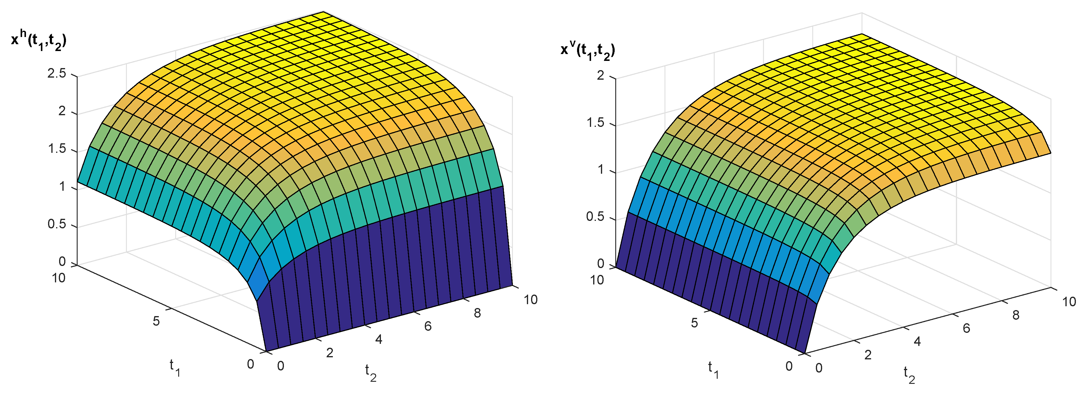
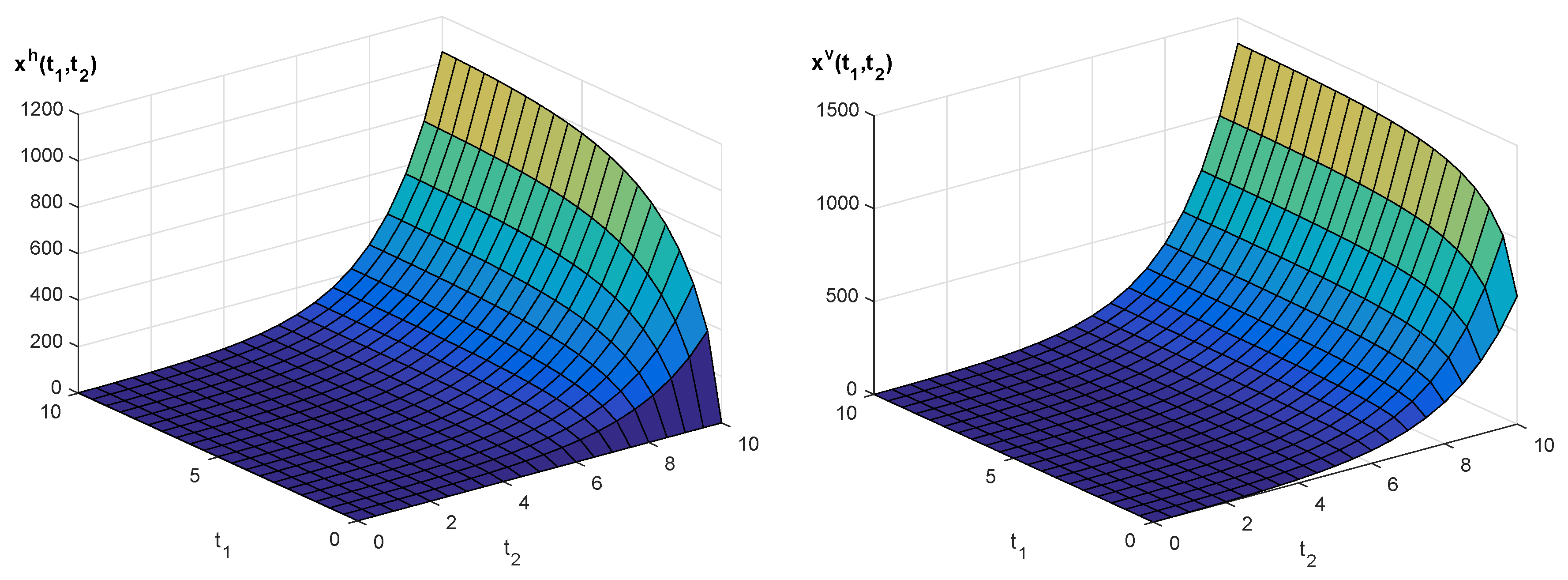
Example 1.

Consider a non-integer order 2D system described by the state Equation (12) with ${\alpha }_1=0.7$, ${\alpha }_2=0.9$ and matrices

$$\begin{array}{cc}\hfill \left[\begin{array}{cc}{A}_{11}& A_{12}\\ A_{21}& A_{22}\end{array}\right]& =\left[\begin{array}{cc}-0.9& 0.7\\ 0.1& a\end{array}\right],\hfill \\ \hfill \left[\begin{array}{c}{B}_1\\ B_2\end{array}\right]=\left[\begin{array}{c}1\\ 1\end{array}\right],C& =\left[\begin{array}{cc}1& 0\\ 0& 1\end{array}\right],D=\left[0\right]\hfill \end{array}$$

(40)

for $a=-0.7$ and $a=0.7$.

Find a step response of the system, i.e., $y(t_1,t_2)$ for $t_1,t_2\ge 0$ and

$$u(t_1,t_2)=H(t_1,t_2)=\left\{\begin{array}{ccccc}0& \mathrm{for}& t_1<0& \mathrm{and}/\mathrm{or}& t_2<0\\ 1& \mathrm{for}& t_1,t_2\ge 0& \end{array}\right.$$

and zero boundary conditions

$$\begin{array}{c}\hfill x^h(0,t_2)=h\left(t_2\right)=0\mathrm{for}{t}_2\ge 0,\\ \hfill x^v(t_1,0)=v\left(t_1\right)=0\mathrm{for}{t}_1\ge 0.\end{array}$$

Note that in this particular case we have

$$y(t_1,t_2)=\left[\begin{array}{c}{x}^h(t_1,t_2)\\ x^v(t_1,t_2)\end{array}\right].$$

The plot of the step response (39) for the 2D system (12) with matrices (40), where $L_1=50$ and $L_2=50$ are shown in Figure 1 for $a=-0.7$ (stable case) and in Figure 2 for $a=0.7$ (unstable case).

7. Concluding Remarks

In this paper, the continuous Roesser type two-dimensional model containing partial non-integer order derivatives described by the Conformable Fractional Derivative definition has been considered and the general solution formula has been derived. CFD system requires only the knowledge of the boundary conditions of Dirichlet type in contrast to the models with Riemann–Liouville definition of fractional-order derivative where the derivatives of boundary conditions should be assumed.

Many different partial differential equations may be expressed by the presented model. Therefore, using the obtained solution, we are able to find a solution formula for this equation. Moreover, the solution is very convenient for numerical computations. Despite the fact that the obtained expression is an infinite sum of matrices and integrals of the boundary conditions and inputs, in practical cases we may bound the higher limits of the sums by some finite numbers depending on the dynamic properties of the system state matrix. The precision of the results in this case is satisfactory, as the expression under the sum decreases rapidly when the indexes of the sum are increasing.

In the paper, the modified Laplace transform has been used to solve the two-dimensional non-integer partial differential equations. It is a very efficient approach, as such transform has similar properties as the classical one-sided Laplace transform. It is well-known that the CFD definition may be expressed using the standard first-order derivative of a function with weighting factors depending on time. This approach leads to the time varying system and the analytical solution becomes more complex and difficult. Therefore, the method presented in this paper is more appropriate to find a formula that describes the general response of the model.

Using the general response formula, we are able to obtain the response of the system for different input functions with arbitrary boundary conditions, especially the system step response, which plays a key role in the study of the dynamics of real-world processes. Based on the solution to the model, the asymptotic stability and other dynamical properties of such systems may be considered.

The presented in the paper results proves that the above considerations can be extended for a general 2D model [7] or for the first and second Fornasini–Marchesini structure models [5,6].