Joint Entity-Relation Extraction via Improved Graph Attention Networks


Abstract
:
1. Introduction
- We designed a new joint model to further the current research on joint entity-relation extraction, and it notably improves upon the traditional methods in the extraction of related information.
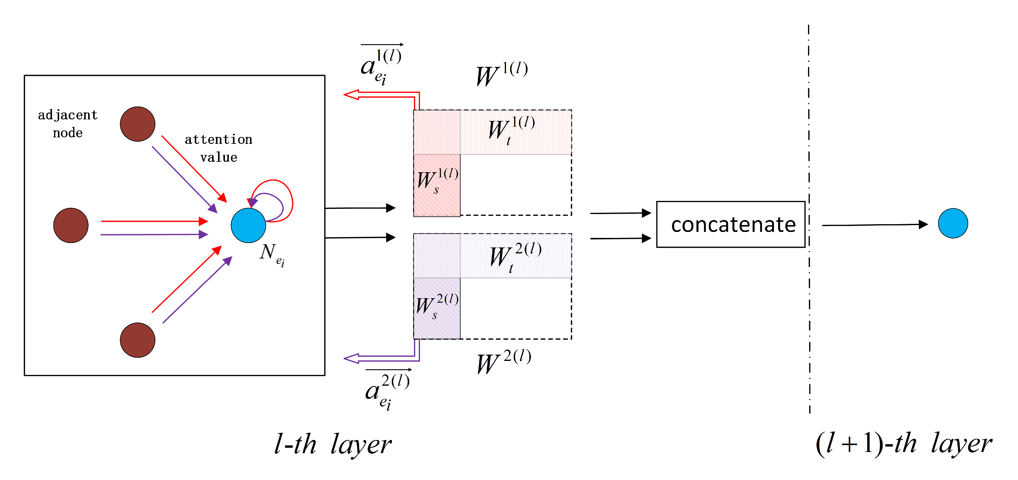
- We introduced the GAT into the domain of joint entity-relation extraction and improved it by designing an efficient multi-head attention mechanism that reduces and shares parameters.
2. Related Work
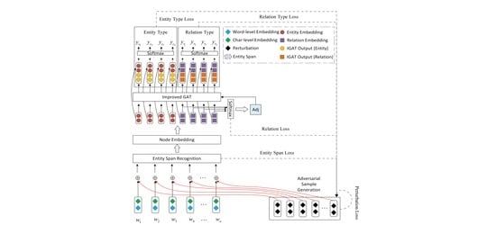
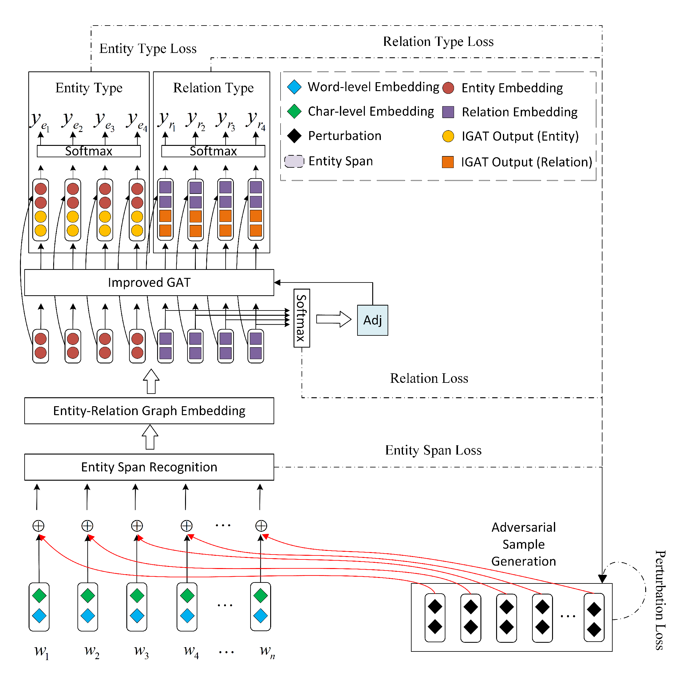
3. Model
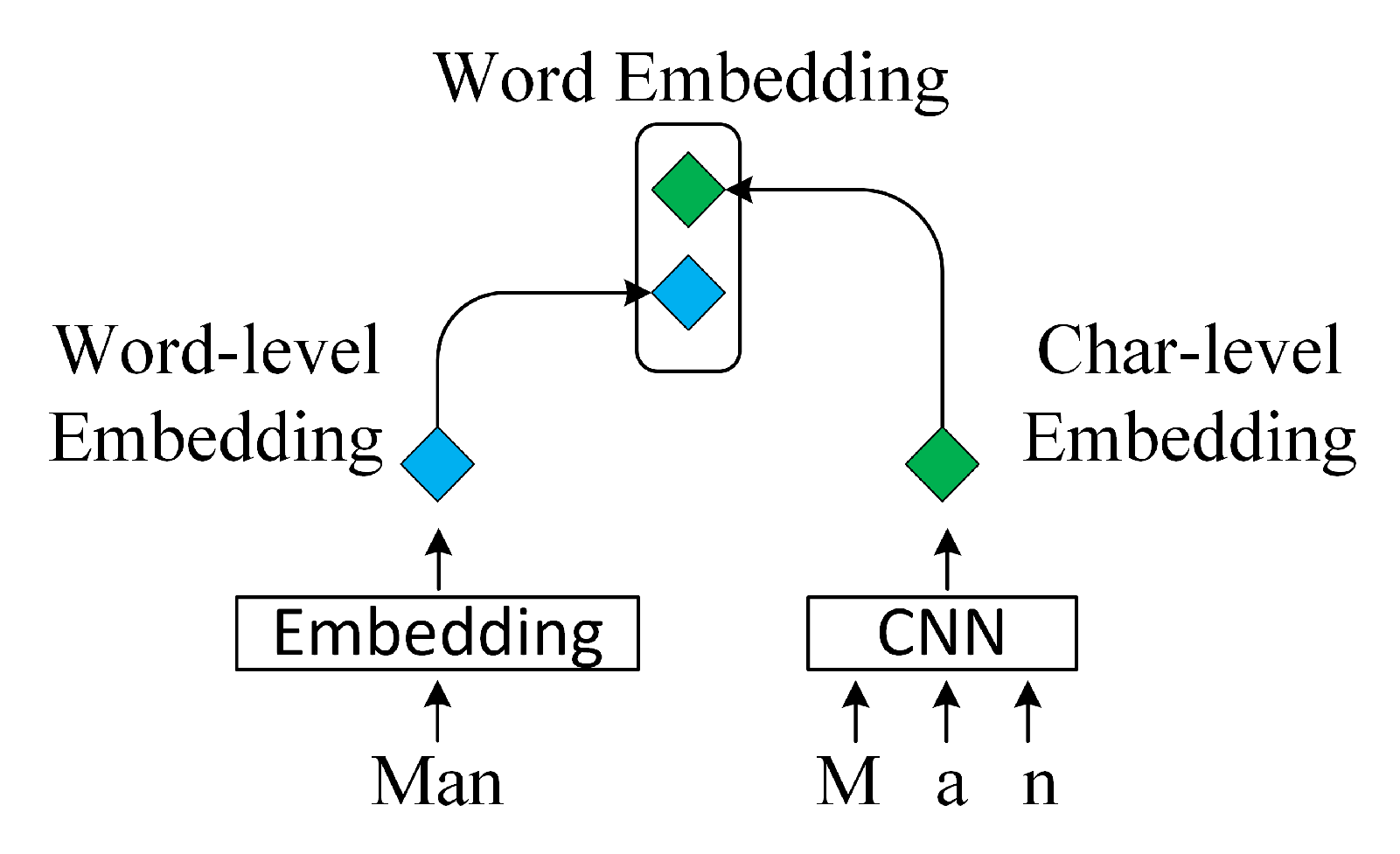
3.1. Word Embedding
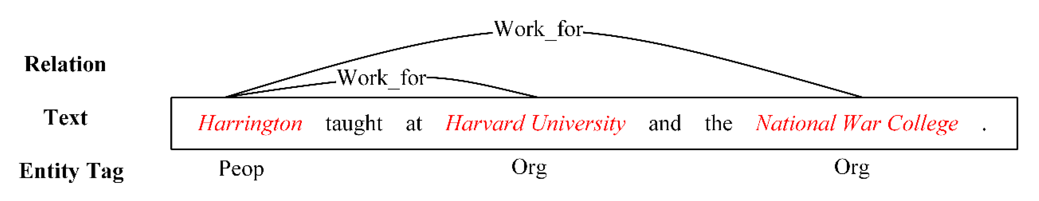
3.2. Entity Span Recognition
3.3. Entity-Relation Graph Embedding
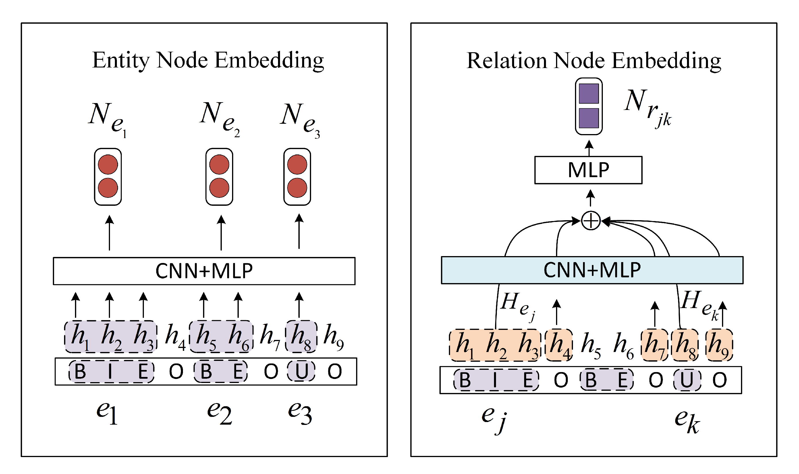
3.3.1. Entity Node Embedding
3.3.2. Relation Node Embedding
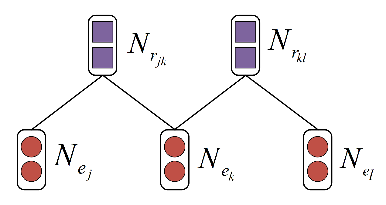
3.3.3. Adjacency Matrix Embedding
- When , we assume that and have a relation with , respectively, i.e., the corresponding position element in A is .
- To capture more information, we add a self-loop to the graph, i.e., the diagonal element in A is .
- All the remaining locations are set to 0.
3.4. Improved Graph Attention Networks
Entity and Relation Classification Tasks
3.5. Adversarial Sample Generation
4. Experiments
4.1. Datasets
4.1.1. CoNLL04
4.1.2. ADE
4.2. Evaluation
4.3. Experiment Setting
4.4. Baseline Models
4.5. Results and Analysis
4.5.1. CoNLL04 Dataset Experimental Results
4.5.2. ADE Dataset Experimental Results
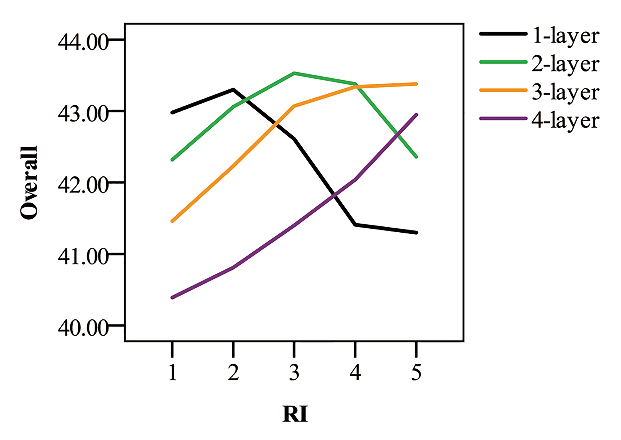
4.5.3. Experiment of Graph Density and IGAT Depth
- Internal factors: the stronger the ability of the graph neural network to differentiate and aggregate node information, the less smooth the information will be after aggregation. Besides, proper parameter size is crucial. These two internal factors determine the depth of the IGAT.
- External factors: in this research, as reflected by model performance, we find that the depth of the IGAT is influenced by the GD, i.e., a deeper IGAT performs better when processing high-density entity-relation graphs.
5. Conclusions
Author Contributions
Funding
Acknowledgments
Conflicts of Interest
References
- Li, Q.; Ji, H. Incremental joint extraction of entity mentions and relations. In Proceedings of the 52nd Annual Meeting of the Association for Computational Linguistics (Volume 1: Long Papers), Baltimore, MD, USA, 22–27 June 2014; pp. 402–412. [Google Scholar]
- Katiyar, A.; Cardie, C. Going out on a limb: Joint extraction of entity mentions and relations without dependency trees. In Proceedings of the 55th Annual Meeting of the Association for Computational Linguistics (Volume 1: Long Papers), Vancouver, BC, Canada, 30 July–4 August 2017; pp. 917–928. [Google Scholar]
- Miwa, M.; Bansal, M. End-to-End Relation Extraction using LSTMs on Sequences and Tree Structures. In Proceedings of the 54th Annual Meeting of the Association for Computational Linguistics (Volume 1: Long Papers), Berlin, Germany, 7–12 August 2016; pp. 1105–1116. [Google Scholar]
- Zheng, S.; Hao, Y.; Lu, D.; Bao, H.; Xu, J.; Hao, H.; Xu, B. Joint entity and relation extraction based on a hybrid neural network. Neurocomputing 2017, 257, 59–66. [Google Scholar] [CrossRef]
- Bekoulis, G.; Deleu, J.; Demeester, T.; Develder, C. Adversarial training for multi-context joint entity and relation extraction. arXiv 2018, arXiv:1808.06876. [Google Scholar]
- Shang, C.; Tang, Y.; Huang, J.; He, X.; Zhou, B. End-to-End Structure-Aware Convolutional Networks for Knowledge Base Completion. U.S. Patent Application No. 16/542,403, 5 March 2020. [Google Scholar]
- Wang, S.; Zhang, Y.; Che, W.; Liu, T. Joint extraction of entities and relations based on a novel graph scheme. IJCAI 2018, 4461–4467. [Google Scholar] [CrossRef] [Green Version]
- Sun, C.; Gong, Y.; Wu, Y.; Gong, M.; Jiang, D.; Lan, M.; Sun, S.; Duan, N. Joint type inference on entities and relations via graph convolutional networks. In Proceedings of the 57th Annual Meeting of the Association for Computational Linguistics, Florence, Italy, 28 July–2 August 2019; pp. 1361–1370. [Google Scholar]
- Hong, Y.; Liu, Y.; Yang, S.; Zhang, K.; Wen, A.; Hu, J. Improving Graph Convolutional Networks Based on Relation-Aware Attention for End-to-End Relation Extraction. IEEE Access 2020, 8, 51315–51323. [Google Scholar] [CrossRef]
- Velickovic, P.; Cucurull, G.; Casanova, A.; Romero, A.; Liò, P.; Bengio, Y. Graph Attention Networks. In Proceedings of the 6th International Conference on Learning Representations, Vancouver, BC, Canada, 30 April–3 May 2018. [Google Scholar]
- Lample, G.; Ballesteros, M.; Subramanian, S.; Kawakami, K.; Dyer, C. Neural Architectures for Named Entity Recognition. In Proceedings of the 2016 Conference of the North American Chapter of the Association for Computational Linguistics: Human Language Technologies, San Diego, CA, USA, 12–17 June 2016; pp. 260–270. [Google Scholar]
- Mathew, J.; Fakhraei, S.; Ambite, J.L. Biomedical Named Entity Recognition via Reference-Set Augmented Bootstrapping. arXiv 2019, arXiv:1906.00282. [Google Scholar]
- Zeng, D.; Liu, K.; Lai, S.; Zhou, G.; Zhao, J. Relation classification via convolutional deep neural network. In Proceedings of the COLING 2014, the 25th International Conference on Computational Linguistics: Technical Papers, Dublin, Ireland, 23–29 August 2014; pp. 2335–2344. [Google Scholar]
- Wang, L.; Cao, Z.; De Melo, G.; Liu, Z. Relation classification via multi-level attention cnns. In Proceedings of the 54th Annual Meeting of the Association for Computational Linguistics (Volume 1: Long Papers), Berlin, Germany, 7–12 August 2016; pp. 1298–1307. [Google Scholar]
- Adel, H.; Schütze, H. Global Normalization of Convolutional Neural Networks for Joint Entity and Relation Classification. In Proceedings of the 2017 Conference on Empirical Methods in Natural Language Processing, Copenhagen, Denmark, 9–11 September 2017; pp. 1723–1729. [Google Scholar]
- Zheng, S.; Xu, J.; Zhou, P.; Bao, H.; Qi, Z.; Xu, B. A neural network framework for relation extraction: Learning entity semantic and relation pattern. Knowl. Based Syst. 2016, 114, 12–23. [Google Scholar] [CrossRef]
- Gupta, P.; Schütze, H.; Andrassy, B. Table filling multi-task recurrent neural network for joint entity and relation extraction. In Proceedings of the COLING 2016, the 26th International Conference on Computational Linguistics: Technical Papers, Osaka, Japan, 11–16 December 2016; pp. 2537–2547. [Google Scholar]
- Bai, C.; Pan, L.; Luo, S.; Wu, Z. Joint extraction of entities and relations by a novel end-to-end model with a double-pointer module. Neurocomputing 2020, 377, 325–333. [Google Scholar] [CrossRef]
- Geng, Z.; Chen, G.; Han, Y.; Lu, G.; Li, F. Semantic relation extraction using sequential and tree-structured LSTM with attention. Inf. Sci. 2020, 509, 183–192. [Google Scholar] [CrossRef]
- Lee, J.; Seo, S.; Choi, Y.S. Semantic relation classification via bidirectional lstm networks with entity-aware attention using latent entity typing. Symmetry 2019, 11, 785. [Google Scholar] [CrossRef] [Green Version]
- Eberts, M.; Ulges, A. Span-based Joint Entity and Relation Extraction with Transformer Pre-training. arXiv 2019, arXiv:1909.07755. [Google Scholar]
- Zhang, J.; He, Q.; Zhang, Y. Syntax Grounded Graph Convolutional Network for Joint Entity and Event Extraction. Neurocomputing 2020. [Google Scholar] [CrossRef]
- Goodfellow, I.J.; Shlens, J.; Szegedy, C. Explaining and Harnessing Adversarial Examples. In Proceedings of the 3rd International Conference on Learning Representations, ICLR 2015, San Diego, CA, USA, 7–9 May 2015. [Google Scholar]
- Ebrahimi, J.; Rao, A.; Lowd, D.; Dou, D. HotFlip: White-Box Adversarial Examples for Text Classification. In Proceedings of the 56th Annual Meeting of the Association for Computational Linguistics (Volume 2: Short Papers), Melbourne, Australia, 15–20 July 2018; pp. 31–36. [Google Scholar]
- Miyato, T.; Dai, A.M.; Goodfellow, I.J. Adversarial Training Methods for Semi-Supervised Text Classification. In Proceedings of the 5th International Conference on Learning Representations, ICLR 2017, Toulon, France, 24–26 April 2017. [Google Scholar]
- Krizhevsky, A.; Sutskever, I.; Hinton, G.E. Imagenet classification with deep convolutional neural networks. Commun. ACM 2017, 60, 84–90. [Google Scholar] [CrossRef]
- Wang, W.C.; Chau, K.w.; Qiu, L.; Chen, Y.b. Improving forecasting accuracy of medium and long-term runoff using artificial neural network based on EEMD decomposition. Environ. Res. 2015, 139, 46–54. [Google Scholar] [CrossRef] [PubMed]
- Pennington, J.; Socher, R.; Manning, C.D. Glove: Global vectors for word representation. In Proceedings of the 2014 conference on empirical methods in natural language processing (EMNLP), Doha, Qatar, 25–29 October 2014; pp. 1532–1543. [Google Scholar]
- Mikolov, T.; Chen, K.; Corrado, G.; Dean, J. Efficient Estimation of Word Representations in Vector Space. arXiv 2013, arXiv:1301.3781. [Google Scholar]
- Ma, X.; Hovy, E. End-to-end Sequence Labeling via Bi-directional LSTM-CNNs-CRF. In Proceedings of the 54th Annual Meeting of the Association for Computational Linguistics (Volume 1: Long Papers), Berlin, Germany, 7–12 August 2016; pp. 1064–1074. [Google Scholar]
- Aleyasen, A. Entity Recognition for Multi-Modal Socio-Technical Systems. Ph.D. Thesis, University of Illinois at Urbana-Champaign, Champaign, IL, USA, 2015. [Google Scholar]
- Zhang, M.; Zhang, Y.; Fu, G. End-to-end neural relation extraction with global optimization. In Proceedings of the 2017 Conference on Empirical Methods in Natural Language Processing, Copenhagen, Denmark, 7–11 September 2017; pp. 1730–1740. [Google Scholar]
- Bekoulis, G.; Deleu, J.; Demeester, T.; Develder, C. Joint entity recognition and relation extraction as a multi-head selection problem. Expert Syst. Appl. 2018, 114, 34–45. [Google Scholar] [CrossRef] [Green Version]
- Li, X.; Yin, F.; Sun, Z.; Li, X.; Yuan, A.; Chai, D.; Zhou, M.; Li, J. Entity-Relation Extraction as Multi-Turn Question Answering. In Proceedings of the 57th Annual Meeting of the Association for Computational Linguistics, Florence, Italy, 28 July–2 August 2019; pp. 1340–1350. [Google Scholar]
- Li, F.; Zhang, Y.; Zhang, M.; Ji, D. Joint Models for Extracting Adverse Drug Events from Biomedical Text. IJCAI 2016, 2016, 2838–2844. [Google Scholar]
- Li, F.; Zhang, M.; Fu, G.; Ji, D. A neural joint model for entity and relation extraction from biomedical text. BMC Bioinform. 2017, 18, 198. [Google Scholar] [CrossRef] [PubMed] [Green Version]
- Zeiler, M.D. Adadelta: An Adaptive Learning Rate Method. arXiv 2012, arXiv:1212.5701. [Google Scholar]


| Dataset | Sentence | Entity | Relation | Entity Type | Relation Type | Training | Validation | Test |
|---|---|---|---|---|---|---|---|---|
| CoNLL04 | 1441 | 1731 | 698 | 4 | 5 | 910 | 243 | 288 |
| ADE | 4271 | 10,652 | 6682 | 2 | 1 | 3417 | 427 | 427 |
| Hyperparameters | CoNLL04 | ADE |
|---|---|---|
| Word-Level Embedding | 100 | 100 |
| Char-Level Embedding | 50 | 50 |
| BiLSTM Layers | 1 | 1 |
| BiLSTM Hidden | 128 | 128 |
| CNN-Kernel Sizes | 2, 3 | 2, 3 |
| CNN-OutputChannels | 25 | 25 |
| MLP | [50, 128] | [50, 128] |
| IGAT Layers | 2 | 3 |
| Attention Heads | 1 | 2 |
| Attention Dimension | 32 | 16 |
| IGAT Hidden | 128 | 64, 64 |
| 0.002 | 0.002 | |
| Learning Rate | 0.3 | 0.3 |
| epoch | 400 | 400 |
| Models | Entity P | Entity R | Entity F1 | Relation P | Relation R | Relation F1 | Overall |
|---|---|---|---|---|---|---|---|
| MLLSTM [32] | - | - | 85.60 | - | - | 67.80 | 76.70 |
| MHS [33] | - | - | 83.04 | - | - | 61.04 | 72.04 |
| MHS-Ad [5] | - | - | 83.61 | - | - | 61.95 | 72.78 |
| MTQA [34] | 89.00 | 86.60 | 87.78 | 69.20 | 68.20 | 68.70 | 78.24 |
| SpERT [21] | 85.78 | 86.84 | 86.25 | 74.75 | 71.52 | 72.87 | 79.56 |
| ERGCN | 86.77 | 81.04 | 83.81 | 73.90 | 61.83 | 67.33 | 75.57 |
| ERGAT | 90.00 | 83.12 | 86.43 | 74.83 | 62.32 | 68.01 | 77.22 |
| ERIGAT-No Ad | 90.07 | 85.02 | 87.47 | 76.63 | 68.14 | 72.14 | 79.81 |
| ERIGAT | 90.04 | 85.57 | 87.75 | 77.06 | 68.79 | 72.70 | 80.22 |
| Models | Entity P | Entity R | Entity F1 | Relation P | Relation R | Relation F1 | Overall |
|---|---|---|---|---|---|---|---|
| CNNE [35] | 79.50 | 79.60 | 79.55 | 64.00 | 62.90 | 63.45 | 71.55 |
| CNN-LSTM [36] | 82.70 | 86.70 | 84.65 | 67.50 | 75.80 | 71.41 | 78.03 |
| MHS [33] | - | - | 86.40 | - | - | 74.58 | 80.49 |
| MHS-Ad [5] | - | - | 86.73 | - | - | 75.52 | 81.13 |
| SpERT [21] | 89.26 | 89.26 | 89.25 | 78.09 | 80.43 | 79.24 | 84.25 |
| ERGCN | 87.34 | 81.92 | 84.54 | 82.37 | 68.64 | 74.88 | 79.71 |
| ERGAT | 90.60 | 82.55 | 86.39 | 83.72 | 71.19 | 76.95 | 81.67 |
| ERIGAT-No Ad | 90.71 | 85.41 | 87.98 | 84.57 | 75.12 | 79.56 | 83.77 |
| ERIGAT | 90.73 | 85.92 | 88.27 | 84.81 | 75.86 | 80.09 | 84.17 |
| RI | GD | NS |
|---|---|---|
| 1 | 85 | |
| 2 | 352 | |
| 3 | 386 | |
| 4 | 448 | |
| 5 | 99 | |
| - | Other | 71 |
Publisher’s Note: MDPI stays neutral with regard to jurisdictional claims in published maps and institutional affiliations. |
© 2020 by the authors. Licensee MDPI, Basel, Switzerland. This article is an open access article distributed under the terms and conditions of the Creative Commons Attribution (CC BY) license (http://creativecommons.org/licenses/by/4.0/).
Share and Cite
Lai, Q.; Zhou, Z.; Liu, S. Joint Entity-Relation Extraction via Improved Graph Attention Networks. Symmetry 2020, 12, 1746. https://doi.org/10.3390/sym12101746
Lai Q, Zhou Z, Liu S. Joint Entity-Relation Extraction via Improved Graph Attention Networks. Symmetry. 2020; 12(10):1746. https://doi.org/10.3390/sym12101746
Chicago/Turabian StyleLai, Qinghan, Zihan Zhou, and Song Liu. 2020. "Joint Entity-Relation Extraction via Improved Graph Attention Networks" Symmetry 12, no. 10: 1746. https://doi.org/10.3390/sym12101746
APA StyleLai, Q., Zhou, Z., & Liu, S. (2020). Joint Entity-Relation Extraction via Improved Graph Attention Networks. Symmetry, 12(10), 1746. https://doi.org/10.3390/sym12101746