Article

Joint Entity-Relation Extraction via Improved Graph Attention Networks

School of Computer Science and Technology, Qilu University of Technology (Shandong Academy of Sciences), Jinan 250353, China
*
Author to whom correspondence should be addressed.
Symmetry 2020, 12(10), 1746; https://doi.org/10.3390/sym12101746
Submission received: 20 September 2020 / Revised: 15 October 2020 / Accepted: 16 October 2020 / Published: 21 October 2020
(This article belongs to the Section Computer)

Abstract

:
Joint named entity recognition and relation extraction is an essential natural language processing task that aims to identify entities and extract the corresponding relations in an end-to-end manner. At present, compared with the named entity recognition task, the relation extraction task performs poorly on complex text. To solve this problem, we proposed a novel joint model named extracting Entity-Relations viaImproved Graph Attention networks (ERIGAT), which enhances the ability of the relation extraction task. In our proposed model, we introduced the graph attention network to extract entities and relations after graph embedding based on constructing symmetry relations. To mitigate the over-smoothing problem of graph convolutional networks, inspired by matrix factorization, we improved the graph attention network by designing a new multi-head attention mechanism and sharing attention parameters. To enhance the model robustness, we adopted the adversarial training to generate adversarial samples for training by adding tiny perturbations. Comparing with typical baseline models, we comprehensively evaluated our model by conducting experiments on an open domain dataset (CoNLL04) and a medical domain dataset (ADE). The experimental results demonstrate the effectiveness of ERIGAT in extracting entity and relation information.

Graphical Abstract

1. Introduction

It is challenging to perform joint named entity recognition (NER) and relation extraction (RE) from unstructured text is in the natural language processing (NLP) and information extraction domains. As an example, given the sentence in Figure 1, the process uses different tags to mark entities and relations during the NER and RE tasks. In this example, Harrington (Peop), Harvard University (Org), and National War College (Org) are three entities: the entity type of Harrington is a “person,” and the entity type of Harvard University or National War College (Org) is an “organization.” The phrase “Work_for” denotes the relation type between Harrington (Peop) and Harvard University (Org) or National War College (Org), respectively.
The traditional entity and relation extraction models can be divided into two main groups based on their different model structures: pipeline models [1] and joint models [2,3,4,5]. The pipeline model has a simple structure and clear logic that treats NER and RE as two independent tasks, where the RE task is located downstream of the NER task. However, the pipeline model can easily cause error forward-propagation, where errors generated in the NER task are passed to the RE task, which limits model performance. In contrast to the pipeline model, the joint model treats NER and RE as two interrelated tasks that do not have a strict upstream and downstream relationship. Thus, errors generated by these two related subtasks can affect and adjust each other. The joint model can achieve better performance than the pipeline model. Therefore, we adopt the joint model as our base model.
Although the graph convolutional network (GCN) has been adopted to the joint extraction task [6,7,8,9], it cannot effectively complete the RE task due to their GCN structure. To improve the effectiveness of the RE task, we introduce an improved graph attention network (IGAT) in our proposed model. The graph attention network (GAT) was first proposed by [10] to solve the semi-supervised node classification problem on a citation network, and it achieved great success. Nevertheless, compared with the citation network, texts contain less entity and relation information, causing the GAT to perform poorly due to high-hop aggregation. Therefore, based on matrix factorization, we improve the graph attention mechanism by sharing the attention parameters and reducing the parameters of the graph convolutional layer. The proposed IGAT has excellent advantages when processing the entity-relation graph, allowing for the efficient extraction of entity and relation information.
In this paper, we embedded the entity and relation information into the entity-relation graph, which is input into the IGAT to capture the entity and relation features. Afterwards, to improve the robustness of our model, we introduced adversarial training (Ad) into our model. In the experiments, we tested our model on two public datasets (CoNLL04 and ADE) in contrast to the baseline models, and the metrics of precision, recall, F1-score, and overall F1 were used. The main contributions of this paper are as follows:
  • We designed a new joint model to further the current research on joint entity-relation extraction, and it notably improves upon the traditional methods in the extraction of related information.
  • We introduced the GAT into the domain of joint entity-relation extraction and improved it by designing an efficient multi-head attention mechanism that reduces and shares parameters.

2. Related Work

The NER task [11,12] and RE task [13,14] are research hotspots for text information extraction. Because the structural defects of the pipeline model limit its model performance, researchers have concentrated on the joint model, which was first proposed by [1] and based on manually designed features. The development of neural networks in the NLP domain provided the ability to extract text features automatically based on neural networks such as the convolutional neural network (CNN) [15,16], the recurrent neural network (RNN) [17,18], the tree-structured long short-term memory neural network (Tree-LSTM) [19], the bidirectional long short-term memory neural network (BiLSTM) [5,20], and the pre-training of deep bidirectional transformers for language understanding (BERT) [21], all of which outperform manually designed feature-based methods. All the above neural networks can successfully extract features from texts. The RNN, LSTM and BERT models have shown significant advantages over the other methods, particularly in the NER task.
However, the above neural network models have no effective module to capture relation information and perform the RE task in complex texts. Research into graph convolutional network (GCN) models has found that GCN can extract node and edge information. Paper [6,7,22] proposed algorithms to obtain relation information based on the graph structure. Later, paper [8] designed a method to construct an adjacency matrix based on binary relation classification, and paper [9] obtained relations based on entity attention. Although these work applied GCN to NER and RE tasks, the GCN structures adopted by these models were simple (consisting of only a 1-layer GCN) and extracted only 1-hop node information, which is insufficient to extract the relation. Additionally, paper [8] used a hard-margin adjacency matrix to aggregate information, which caused over-smoothing and limited the expressive ability of the GCN.
Adversarial training has been widely used as a method to improve model robustness. This technique adds tiny perturbations and has been applied to the NLP domain. At present, many methods of adversarial training [23,24,25] have been proposed in the NLP domain. Paper [23] proposed a method for generating adversarial samples using simplified calculations that reduced the random noise caused by the dropout operation.
To address the insufficient capacity of extraction entity and relation information, We improve and redesign the existing model. From the models mentioned above, our model adopts BiLSTM for entity span recognition and uses a CNN [26] and a multi-layer perceptron (MLP) [27] to obtain the graph embedding. Then, we input the entity-relation graph into the IGAT, which is designed in this paper to enhance the ability of the GAT to extract relation information and mitigate over-smoothing with a simple and efficient multi-head attention mechanism that reduces and shares parameters. To improve the robustness of our method, we adopted adversarial training to generate samples [23]. Besides, we also designed experiments to explore the relation between graph density and the depth of the IGAT.

3. Model

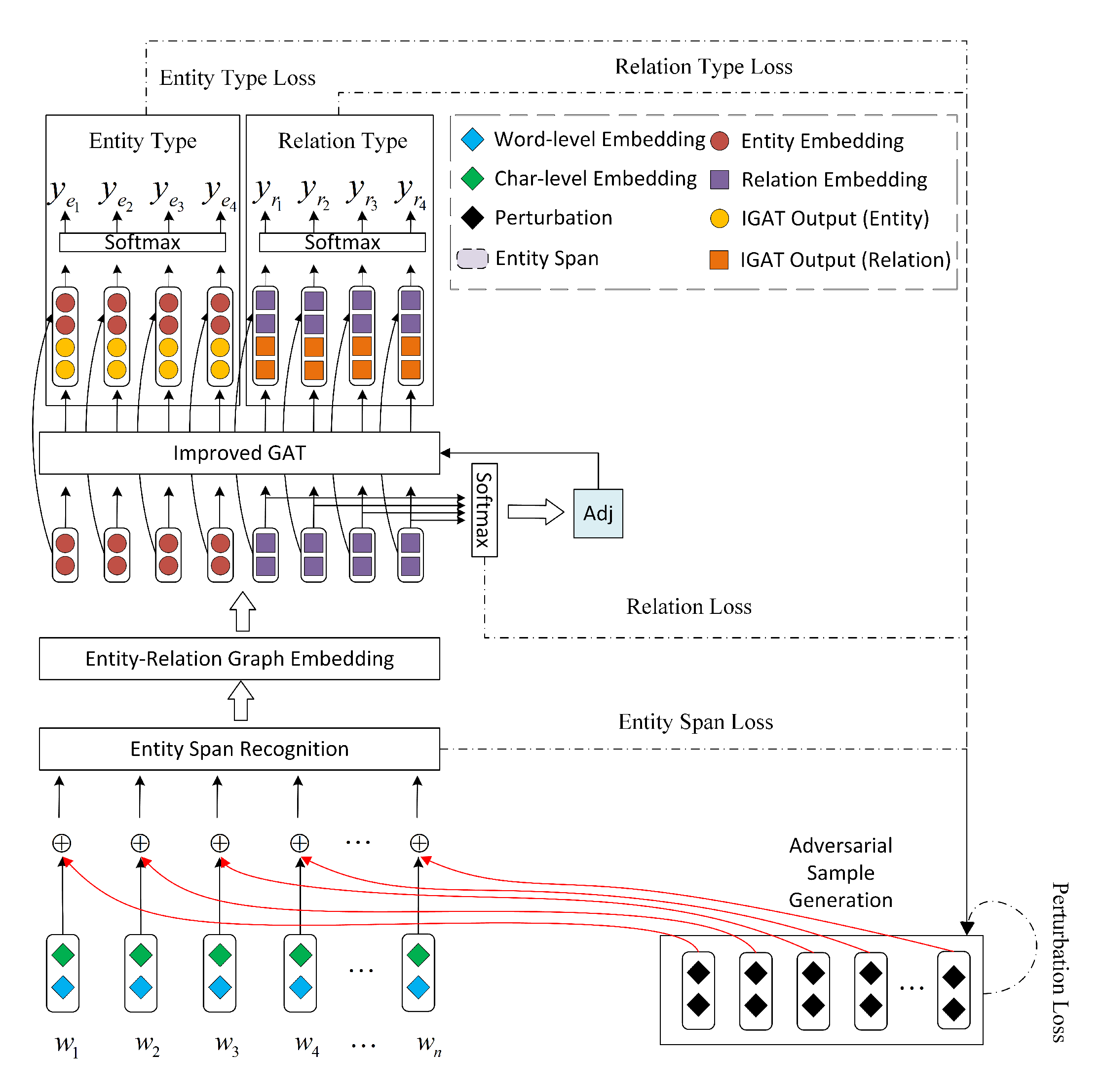
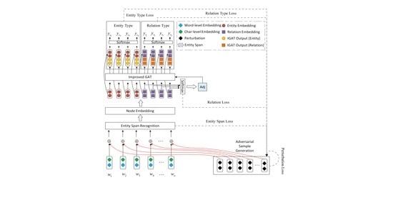
The structure of the Entity-Relations via Improved Graph Attention networks (ERIGAT) is shown in Figure 2. First, a word vector representation is obtained through the word embedding module and then input into the entity span recognition module (BiLSTM layer) to recognize entity spans. The loss of the entity span is calculated after identifying the entity span. Next, the graph embedding module uses the entity span and the output of the BiLSTM layer to obtain an entity-relation graph. Then, the entity nodes, relation nodes, and adjacency matrix are fed into the IGAT, which extracts the entity and relation information. Finally, after the extracted information is concatenated with the node embedding output, we can classify the entity types and the relations types.
Among the modules, the IGAT is the core of the innovation. The rest of the modules mostly use existing methods.
After the first forward propagation, the parameters are fixed. We obtain the adversarial samples based on the first forward propagation loss and add adversarial samples to the word embedding. Then, after the second forward propagation, the loss values of the two forward propagations are accumulated, and the parameters are optimized through backpropagation.

3.1. Word Embedding

The word vector representation is composed of word-level embedding and character-level (char-level) embedding, and the process of word embedding is illustrated in Figure 3.
Given a sentence w = { w 1 , , w n } as a sequence of tokens (where w i is a word), the pre-trained word embedding model (GloVe) [28] can obtain each unique word as a vector (the word-level embedding), then the word2vec model [29] can get the semantic information of words from these vectors.
Besides, to capture the word morphological information, the method proposed by [30] is adopted to extract character information using a CNN model. The character information includes prefix and suffix information of words and other morphological information. For example, suppose “water” is contained in a word. Based on the different subordinate positions of “water” in the word, we can distinguish among specific entity types. For example, in CoNLL04, the entities Watergate and Goldwater belong to the “Other” type and the “Peop” type, respectively. In ADE, the prefix “hypo” can specify an adverse-effect entity such as hypophosphatemia or hyponatremia. Therefore, char-level embedding provides helpful auxiliary information for word vector representation.
In this study, we comprehensively consider both of word-level and char-level embedding methods and concatenate them to obtain a vector representation for each word.

3.2. Entity Span Recognition

The proposed model obtains the entity span based on the output of the BiLSTM and the BIEOU scheme.
Our proposed model uses the BIEOU scheme [31] to mark the entity span, where “B”, “I”, “E”, and “O” represent the beginning, inside, end, and outside of the entity span, respectively. The “U” in BIEOU represents an entity that is a single word. Given two entities, New York City (Loc) and Lincoln (Peop), we can mark them with BIE and U, respectively. The entity span recognition structure is illustrated in Figure 4.
For sentence w = { w 1 , , w n } , we can obtain the embedding matrix of the sentence X = { x 1 , , x n } (where x i is the vector representation of w i after word embedding). Then, we input X into the BiLSTM to extract the entity span information, which is calculated as follows:
h i = BiLSTM ( x i ; θ s p a n ) ,
where h i is the concatenation of a forward and a backward context feature vector and x i is extracted by the BiLSTM with the parameters θ s p a n . Then, we can predict the entity span tags t i ^ corresponding to the word w i as follows:
P ( t i ^ | w ) = softmax ( W s p a n h i ) ,
where W s p a n is the weight parameter of the entity span. Given sentence w and its entity span target tags, t = { t 1 , , t | w | } , the entity span recognition loss is formulated as follows:
L s p a n = 1 | w | i = 1 | w | log P ( t i ^ = t i | w ) .

3.3. Entity-Relation Graph Embedding

To extract entity and relation information with the IGAT, we need to embed the obtained entity vector into an entity-relation graph according to the entity span information.

3.3.1. Entity Node Embedding

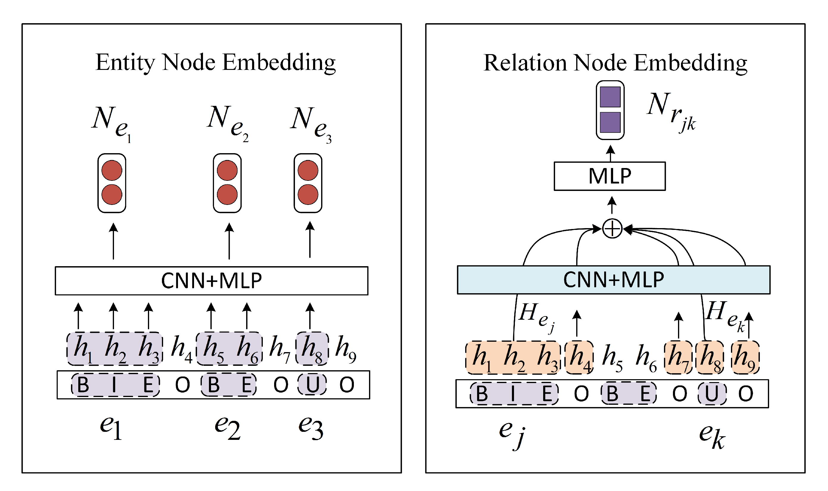
The entity node embedding structure is shown in the left part of Figure 5. We define an entity as e and a set of entities as ε ^ in each sentence. Based on the entity span tags recoginzed in the last step t ^ , we can obtain the range of the entity. For example, in the left part of Figure 5, ε ^ e x a m p l e = e 1 , e 2 , e 3 , where e 1 = h 1 , h 2 , h 3 , e 2 = h 5 , h 6 , and e 3 = h 8 . We use a CNN (a single convolution layer with a max-pooling layer) with a MLP to obtain the entity node embedding N e R d n o d e .

3.3.2. Relation Node Embedding

We define r j k as the relation between entity e j and entity e k . When initializing the relation nodes, we assume that there is a potential relation between any two entities in a sentence (i.e., the number of potential relations in each sentence is | ε ^ | ( | ε ^ | 1 ) 2 ). To capture the impact of contextual information on the relation, we need to embed not only information regarding the entity itself but also its contextual information. For example, given a sentence “Rome is in Lazio province,” which contains the entities Rome (Loc) and Lazio (Loc), it is difficult to extract the relation between the two entities without considering the contextual information and the lack of prior knowledge. Instead, we can extract the relation between Rome and Lazio as “Locate_in” based on the contextual information provided by “in” and “province”.
Motivated by this idea, we use entity node embedding N e j , N e k and the context feature vectors of the two entities. Similarly, we build context features by running another CNN with MLP. Finally, the entities node embedding and context feature vectors are concatenated to a single vector. We apply an MLP on the single vector to get relation node embedding N r j k R d n o d e .

3.3.3. Adjacency Matrix Embedding

To predict whether a definite relation exists between two entities, we define a binary relation tag b with a value in { 0 , 1 } , where 0 means there no relation exists between the two entities and 1 means that a relation exists between the two entities. We also define the binary relation tag b ^ for prediction. The probability of b ^ is calculated as follows:
P ( b ^ | r j k , w ) = softmax ( W a d j N r j k ) ,
where W a d j is a weight parameter. The loss value is calculated as follows:
L r e l = r j k log P ( b ^ = b | r j k , w ) # c a n d i d a t e r e l a t i o n r j k .
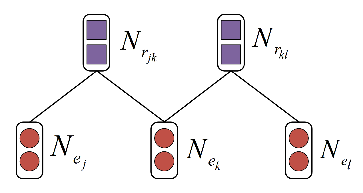
To obtain the entity-relation graph, we construct a symmetric relation between entity nodes and relation nodes. For example, Figure 6 depicts the symmetric relation among N e j , N e k and N r j k . Then, we obtain the adjacency matrix A of the entity-relation graph using the following method:
  • When P ( b ^ = 1 | r j k , w ) 0.5 , we assume that N e j and N e k have a relation with N r j k , respectively, i.e., the corresponding position element in A is 1.0 .
  • To capture more information, we add a self-loop to the graph, i.e., the diagonal element in A is 1.0 .
  • All the remaining locations are set to 0.

3.4. Improved Graph Attention Networks

Because the typical neural network models have no advantage in performing the RE task in complex texts, to promote the effectiveness of the RE task, we applied the method proposed by [8] to introduce the GCN into entity and relation extraction experiments, which is calculated as follows:
N G ( l + 1 ) = σ ( A ^ N G ( l ) W ( l ) ) ,
where A ^ = D 1 2 A D 1 2 and D is the diagonal node degree matrix with D i i = j A i j . N G R n n o d e × d n o d e contains all the embedded nodes, where N G ( 0 ) = N G , n n o d e is the number of nodes in the entity-relation graph and d n o d e is the node feature dimension. We define L as the number of layers in the GCN, l as the current layer in the GCN, and W ( l ) as the convolutional parameter for the l -th GCN layer. In experiments, we found this GCN model difficult to distinguish the aggregated node information because of its hard-margin adjacency matrix, which can easily lead to over-smoothing. Moreover, unlike the GCN used in a citation graph, in which the feature dimension gradually decreases as the GCN layers deepen, in the entity and relation extraction tasks, we need to preserve the same feature dimension for each GCN layer in the entity-relation graph to obtain the feature contribution of all the entities and relations. However, this approach would result in an enormous number of parameters in the GCN due to the value of L × d n o d e 2 .
To mitigate over-smoothing by differentiating aggregation information, we introduce a GAT into the joint entity and relation extraction domain for the first time. The attention coefficient of the GAT can be obtained as follows:
E d g e i j = ϕ ( [ W N e i | | W N e j ] ) ,
where N e i is the node embedding of entity e i and N e j is one of the 1-hop adjacent nodes of N e i , and W is a trained matrix. The symbol | | denotes concatenation, and ϕ ( · ) is a mapping vector. We define C a t as the number of attention heads and c as current attention head, where 1 < = c < = C a t and c is an integer. Then, we can obtain the attention coefficient vector E d g e i and calculate the attention as follows:
a i = softmax ( E d g e i ) ,
where a i is the attention vector for N e i with 1-hop adjacent node. We can use the value of a i to set the corresponding position element in A and obtain the attention adjacency matrix A ^ c ( l ) . For each head attention in each layer of the GAT, we initialize the trained matrix W c ( l ) . The GAT can be formulated as follows:
N G ( l + 1 ) = | | c = 1 C a t σ ( A ^ c ( l ) N G ( l ) W c ( l ) ) .
Although the GAT can differentiate aggregation information and mitigate over-smoothing to some degree with the attention mechanism, the sample aggregation can only be used for message passing. Hence the internal relationship in the node features is ignored. Moreover, with the enormous number of parameters and node features sparsity, the GCN or GAT causes over-fitting. According to the above analysis, over-smoothing and over-fitting limit the depth of both the GCN and the GAT in aggregating node information, so that they can only aggregate 1-hop node information in the entity-relation graph, which is insufficient for completing the entity and relation extraction task. Furthermore, a 1-layer GCN or GAT performs poorly in extracting high-dimensional features.
To solve these problems (over-smoothing, lack of internal relationship in node features and over-fitting caused by the sparsity), we design a new multi-head attention mechanism for the GAT, named the improved graph attention network (IGAT), to extract the information of entity and relation more efficiently. Using matrix factorization, we can capture relationships in nodes and internal relationships in node features by mapping high-dimensional sparse vectors to low-dimensional dense vectors. Furthermore, based on the attention parameters’ sharing with the convolutional layer, we can use fewer parameters than the GCN and the GAT to obtain the same attention structure in each graph convolutional layer. To sum up, now we can use deeper graph convolutional layers than the GCN and the GAT to comprehensively extract the entity and relation information by enhancing feature extraction capabilities and reducing parameters.
In IGAT, we can factorize the GAT convolutional matrix W c ( l ) R d n o d e × d c ( l ) to pre-trained attention parameter matrices W s c ( l ) R d n o d e × d a t c ( l ) and W t c ( l ) R d a t c ( l ) × d c ( l ) , where d a t c ( l ) is the attention dimension. The convolutional layer matrix W c ( l ) ’s factorization formulation is as follows:
W c ( l ) = W s c ( l ) W t c ( l ) .
For each convolutional layer of the IGAT, we use matrix W s c ( l ) to share the attention parameters with the convolutional layer because the matrix W s c ( l ) retains the pre-trained information after the attention mechanism and reduces the node feature sparsity due to the reduction of the matrix dimension. Furthermore, with the matrix multiplication of matrix W s c ( l ) and W t c ( l ) , we can keep the same feature dimensions of each convolutional layer with GAT. Meanwhile the use of the matrix W s c ( l ) and W t c ( l ) instead of W c ( l ) can map dense node features to the new feature space to extract deeper level node information. For example, given a matrix W c ( l ) R 128 × 128 , which can be fitted by W s c ( l ) R 128 × 32 W t c ( l ) R 32 × 128 and the parameter quantity has obviously reduced. Unlike the traditional eigenvalue matrix factorization, IGAT need not calculate the matrix factorization loss since the convolutional matrix W s c ( l ) and W t c ( l ) ’s parameters are updated dynamically through back propagation of the IGAT network. To obtain the attention parameters matrix W s c ( l ) and attention adjacent matrix E G c ( l ) R n n o d e × n n o d e in IGAT which is composed of attention values, first IGAT defines Q e i as a matrix composed of N e i and its 1-hop adjacent node. Then, instead of Formula (7) in GAT, the IGAT calculates the attention value matrix for each head attention as follows:
a e i c ( l ) = softmax ( | | ReLU ( Q e i W s c ( l ) ) | | 2 ) ,
where | | · | | 2 is the row 2-norm and a e i c ( l ) is the attention vector between N e i and its 1-hop adjacent node. Next, we introduce degree information into the GAT and obtain an attention adjacency matrix E G c ( l ) by mapping each node attention value to corresponding positions in A. Afterwards, we can get the normalized symmetric adjacency matrix E G c ( l ) as follows:
E ^ G c ( l ) = D 1 2 E G c ( l ) D 1 2 ,
where D i i = j E G c ( l ) i j . Based on the above analysis, we reach the following IGAT convolutional formula:
N G ( l + 1 ) = | | c = 1 C a t σ ( E ^ G c ( l ) N G ( l ) W s c ( l ) W t c ( l ) ) .
Finally, after the information extraction of the IGAT network, we obtain the feature matrix in the last layer as Z = N G ( L ) .
The multi-head attention mechanism that aggregates node information and shares attention parameters with the convolutional layer is shown in Figure 7.
Compared with the GCN and the GAT, the IGAT improves the ability to differentiate and aggregate information, which mitigates over-smoothing. In addition, we reduce the parameters of the GAT by using row 2-norm to obtain the attention coefficient instead of ϕ ( · ) and by matrix factorization which shares the attention mechanism parameters with the convolutional layers. Using matrix factorization, we can extract the internal relationship in node features and reduce node features sparsity. This approach of IGAT allows for the deeper layers of the IGAT in the entity-relation graph, i.e., it can aggregate multi-hop node information, which improves the ability to extract relation information.

Entity and Relation Classification Tasks

We concatenate the feature matrix Z (output by the IGAT) with the input matrix N G (input into the IGAT) to obtain the feature matrix F for the classification task. Then, we define F e j as the feature vector of entity e j and F r j k as the feature vector of relation r j k . We define the target tags of entities and relations as y e and y r , respectively, and the predicted tags of entities and relations are y e ^ and y r ^ , respectively. The entity tags and relations tags can be formulated as follows:
P ( y e ^ | e j , w ) = softmax ( W e n t F e j ) ,
P ( y r ^ | r j k , w ) = softmax ( W r e l F r j k ) ,
where W e n t and W r e l are weight parameters. Finally, the entity and relation loss functions can be written as follows:
L e T y p e = 1 | ε ^ | e j ε ^ log P ( y e ^ = y e | e j , w ) ,
L r T y p e = r j k log P ( y r ^ = y r | r j k , w ) # c a n d i d a t e r e l a t i o n r j k .

3.5. Adversarial Sample Generation

We define the loss of the model as L J o i n t ( X ; θ ) after the first forward propagation, where L J o i n t ( X ; θ ) = L s p a n + L r e l + L e T y p e + L r T y p e , and θ denotes the model parameters. To enhance model robustness, we follow the method proposed in [23] by adding tiny perturbations to the samples for adversarial training. We define η a d as the perturbation added to the samples, while θ ^ is a copy of the parameters θ in the current model, and θ is a fixed parameter set (i.e., the error in this back propagation does not update the parameters). The perturbations are formulated as follows:
η a d = λ g | | g | | ,
where g = X L J o i n t ( X ; θ ^ ) and λ is a small bounded norm treated as a hyperparameter. Similar to [5], we define λ = α D X , where α is a perturbation parameter (set manually), and D X is the feature dimension of X. The loss L J o i n t ( X + η a d ; θ ^ ) of the second forward propagation is obtained by adding the perturbation to X. Considering the losses of both forward propagation steps, we obtain the final loss L F i n a l = L J o i n t ( X ; θ ) + L J o i n t ( X + η a d ; θ ^ ) . Then, we update model parameters θ with L F i n a l to complete the parameter adjustment process.

4. Experiments

In the experiments, we applied our ERIGAT method to an open domain dataset (CoNLL04) and a medical domain dataset (ADE), and we evaluated the results with the previously proposed baseline models to verify the validity of ERIGAT.

4.1. Datasets

We applied our ERIGAT method to accomplish the NER and RE task using data from the CoNLL04 and ADE datasets. The size of ADE is significantly larger than that of CoNLL04, so we chose these two data sets of different sizes for the experiment.

4.1.1. CoNLL04

As shown in Table 1 (CoNLL04 in Table 1), CoNLL04 contains 1441 sentences, 1731 entities, and 698 relations. There are four entity types (“Organization”, “Person”, “Location", and “Other”) and five relation types (“Kill”, “Live_in”, “Located_in”, “OrgBased_in”, and “Work_for”). We divided the CoNLL04 dataset using the division method reported in [5,32,33,34] making the number of sentences in the training, verification, and test sets 910, 243, and 288, respectively.

4.1.2. ADE

The original ADE dataset contains 6821 sentences, but many are repeats. To obtain data information more efficiently, we deduplicated the dataset and unified the entities and relations in duplicate sentences into one sentence. We also removed approximately 130 relations with overlapping entities. For example, lithium is a drug related to lithium intoxication. As shown in Table 1 (ADE in Table 1), after preprocessing, ADE included 4271 sentences, 10,652 entities, and 6682 relations. There are two entity types (“Drugs” and “Adverse_effects”) and one relation type (“Effect”). We followed the division method in [5,33,35,36] to divide the ADE dataset, and the numbers of sentences in the training, validation, and test sets were 3417, 427, and 427, respectively.

4.2. Evaluation

In this study, we used “Strict” standard to evaluate the model results. For the NER task, “Strict” means that a predicted entity is judged to be correct only if both the entity span and the entity type are correct. For the RE task, “Strict” means that the predicted relation is judged as correct only if both the entity span and the relation type are correct. For example, given an entity and relation <Rocky Mountains, Located_In, Montana>, the Rocky Mountains is judged to be correct if the entity span words “Rocky” and “Mountains” are selected, and the corresponding entity type is “Location”. The relation between the two entities is determined to be correct only if both Rocky Mountains and Montana are selected, and the relation type is “Located_in”.
To comprehensively evaluate our model, we adopted precision (P), recall (R), F1-score and overall F1-score as metrics to evaluate the results. Here, O v e r a l l = F 1 e + F 1 r 2 , where F 1 e is the F1-score of the NER task, and F 1 r is the F1-score of the RE task.

4.3. Experiment Setting

Table 2 lists the hyperparameter settings of the ERIGAT model when optimal performance was achieved for the two datasets.
The encoding dimensions for the word-level and char-level embeddings are 100 and 50, respectively.
We obtain a word encoding dimension of 150 after concatenation. We set the number of hidden layers of the BiLSTM to 1 and the hidden layer dimension to 128.
In the proposed model, a CNN configured with the same parameters is used to extract information. The number of convolution kernels is 2, with sizes of 2 and 3, respectively, and the output channel is 25. For the MLP layer, which constructs the entity and relation nodes, we set the input dimension to 50 and the output dimension to 128.
In particular, due to the different graph scales constructed by CoNLL04 and ADE, we adopted different parameter settings when using the IGAT model. For CoNLL04, we set the number of the IGAT layers to 2, the number of attention heads to 1, the attention dimension to 32, and the dimension of the IGAT hidden layer to 128. For ADE, we set the number of the IGAT layers to 3, the number of attention heads to 2, the attention dimension to 16, and the dimensions of IGAT hidden layer to 64 and 64.
For the adversarial sample generation, we set the perturbation parameter α to 0.002. Finally, we adopted AdaDelta [37] to optimize the parameters, and the learning rate was set to 0.3.

4.4. Baseline Models

We compared our ERIGAT model with several baseline models in different categories, including SpERT, MLLSTM, MHS, MHS-Ad, MTQA, CNNE, and CNN-LSTM, each of which is described below.
SpERT: This model [21] introduces the pre-trained Bert model as the core for joint entity recognition and relation extraction.
MLLSTM: This is a multi-layer LSTM (MLLSTM) model [32] that performs end-to-end RE based on globally optimized features. This model uses multi-layer LSTM to extract entity and relation features and introduces an external syntax analyzer to integrate sentence information.
MHS: The multi-head selection (MHS) model [33] does not rely on NLP tools and manual features. The use of the LSTM to extract features from the embedded word representation transforms the NER and RE tasks into a multi-head selection problem.
MHS-Ad: The multi-head selection with adversarial training (MHS-Ad) model [5] introduces adversarial training into the MHS model to enhance model robustness.
MTQA: The multi-turn QA (MTQA) model [34] uses a multi-turn question answering mechanism that transforms the NER and RE tasks into a context. The MTQA model introduces machine reading comprehension to extract information from text.
CNNE: The CNN extractor (CNNE) model [35] is a discrete joint model that improves CNN model performance through information integration methods. The CNNE model uses a CNN-based feature extractor to extract text information.
CNN-LSTM: Based on the CNNE model, the CNN-LSTM model [36] introduces an LSTM that extracts text information from the CNN output and optimizes the model parameters by sharing parameters.
Besides, to illustrate the advantages of the IGAT approach in extracting entities and relations, we devised a comparison experiment that substitutes the original GCN and original GAT models for the IGAT in the complete ERIGAT model, and these variations of ERIGAT are named ERGCN and ERGAT, respectively. Moreover, to verify the effectiveness of adversarial training, we also test the proposed model without adversarial sample generation part, named ERIGAT-No Ad.

4.5. Results and Analysis

Full results and analysis for the performance of our model, as well as other recent work, are shown below.

4.5.1. CoNLL04 Dataset Experimental Results

Table 3 lists the experimental results of the ERIGAT model and the baseline models for the CoNLL04 dataset. The experimental results show that using only an LTSM (MLLSTM, MHS, and MHS-Ad) to extract entity and relation information fails to achieve high performance, and the overall value reaches only 76.70. In particular, with respect to relation information extraction, the LSTM performance is poor. It is challenging for LSTM to deal with relation information above the entity level. Meanwhile, although the overall value of MTQA is improved to 78.24 due to its multi-turn question answering mechanisms, this improvement stems mainly from the NER portion, which suggests that the model’s ability to process relation information is still unstable. Benefits from the huge semantic information in Bert, the SpERT can achieve better performance in entity and relation extraction tasks.
Moreover, compared with MHS and MHS-Ad, ERGCN (1-layer GCN) improves the ability to extract relation information. Although its Entity F1 value is similar to MHS and MHS-Ad, its Relation F1 value increases by approximately 6, which indicates that ERGCN is useful for extracting relation information to some extent. ERGAT (2-head attention and 1-layer GCN) uses differentiated aggregation node information by the attention mechanism and improves the overall performance with a value of 77.22. Compared with ERGAT, ERIGAT (1-head attention and 2-layer GCN) further improves the Entity F1 and Relation F1 values and achieves the best performance of any model, which suggests that ERIGAT aggregates node information better than other models as it deepens the layers of the IGAT by improving the attention mechanism. In addition, the extracted information is not limited to 1-hop adjacent nodes. Thus, the IGAT can extract more in-depth information from additional nodes through the deeper model layers. Compared with SpERT, the ERIGAT can achieve higher performance with less semantic information, which shows that the ERIGAT is strong to extract entity and relation information. In short, the ERIGAT processes entity and relation information more effectively than other models, which achieves the best overall performance at 80.22.

4.5.2. ADE Dataset Experimental Results

Table 4 lists the experimental results of the proposed ERIGAT model and baseline models for the ADE dataset. The results show that both the CNN and the LSTM are good at extracting entity information (word information and context information) in sentences but are poor at extracting relation information. In addition, in terms of performance improvement, the Relation F1 value of the ERIGAT model outperforms those of MHS and MHS-Ad by approximately 10 on CoNLL04 (5 relation types) and 3∼4 on ADE (1 relation type). This suggests that the ERIGAT model is better at processing the complex relation types in entity-relation graphs. Additionally, the entity-relation graph embedded for ADE is larger than that for CoNLL04, which causes the number of attention heads and layers of the IGAT to increase. Since ADE is a medical dataset, only ∼73% (CoNLL is ∼97%) of the words can be found in GloVE. In this case, compared with SpERT (∼79%), the ERIGAT is not high in terms of Entity F1 due to less semantic information is used. Although the entity F1 is lower than SpERT, our relation F1 still exceeds SpERT and other baseline models, which suggests that our new multi-head attention mechanism is strong in extracting relation information. Comprehensive consideration of overall value, the ERIGAT has achieved competitive performance.
Meanwhile, considering the results of the model on the CoNLL04 and ADE datasets, we can conclude that the performance of ERIGAT (CoNLL04 is 80.22% and ADE is 84.17%) is better than ERIGAT-No Ad (CoNLL04 is 79.81% and ADE is 83.77%), which reflects that increasing the robustness of the model by adversarial training can improve the performance of the ERIGAT model. Furthermore, compared with ERGAT (CoNLL04 is 77.22% and ADE is 81.67%), the performance of ERIGAT has been significantly improved, which suggests that the IGAT is effective.

4.5.3. Experiment of Graph Density and IGAT Depth

Moreover, we also designed an ERIGAT experiment on entity-relation graphs with different graph densities. We define ρ G as the graph density, which is formulated as follows:
ρ G = 2 × N u m b e r r N u m b e r e + N u m b e r r ,
where N u m b e r e denotes the number of entity nodes, and N u m b e r r denotes the number of relation nodes.
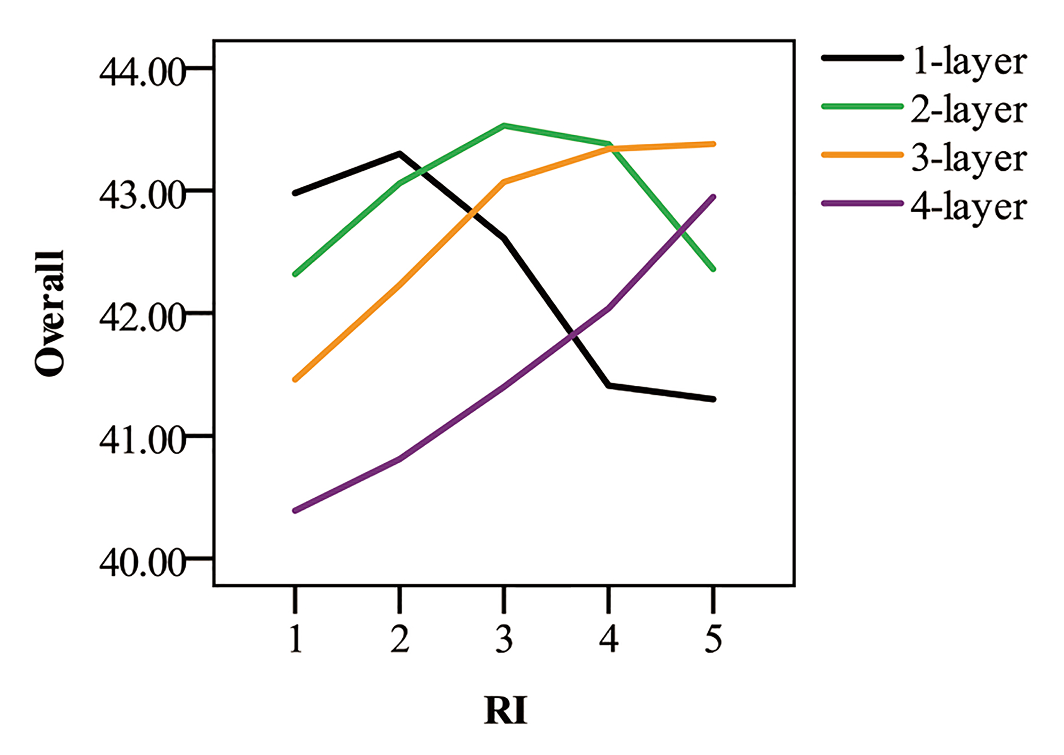
Table 5 lists the number of sentences in CoNLL04 (where the average graph density is 0.57) at different graph density intervals. We set the range ID (RI) as the serial number of each interval and graph density (GD) as the interval density with a step size of 0.15. NS is the number of sentences in the corresponding interval. To ensure consistency for the number of experimental sentences, we randomly selected 85 sentences in each interval, including 61 for training, 11 for verification and 13 for testing. Then, we set up four sets of comparative experiments, in which the number of attention heads in the graph was fixed to 1 and the number of IGAT layers was varied from 1 to 4. Subsequently, we calculated the average values for five experiments.
The results are shown in Figure 8. We find that the IGAT (1-layer) is suitable for extracting data at low graph densities, i.e., entity-relation graphs with sparse relations. However, as the number of relations increases, it becomes difficult for a 1-layer IGAT to extract node information from high-hop neighborhoods, resulting in performance degradation. In contrast, a deeper IGAT, such as an IGAT (4-layer) tends to experience over-smoothing when repeatedly aggregating low-hop node information, resulting in poor performance. However, for high-hop adjacent nodes, the deeper IGAT can capture more node information. Consequently, the model performance gradually improves as the GD increases. Moreover, the IGAT (2-layer) performs best in interval 3, with a density close to the average density of CoNLL04 (0.57). In contrast, the IGAT (3-layer) performs best in interval 4, with a density close to the average density of ADE (0.77), which is consistent with the experimental results on CoNLL04 and ADE.
Combined with the above analysis, we can find the number of layers (network expression capacity) of an IGAT processing the entity-relation graphs is affected by the following factors:
  • Internal factors: the stronger the ability of the graph neural network to differentiate and aggregate node information, the less smooth the information will be after aggregation. Besides, proper parameter size is crucial. These two internal factors determine the depth of the IGAT.
  • External factors: in this research, as reflected by model performance, we find that the depth of the IGAT is influenced by the GD, i.e., a deeper IGAT performs better when processing high-density entity-relation graphs.

5. Conclusions

In this paper, we proposed a new joint model named ERIGAT, that introduces the GAT into the entity-relation joint extraction domain for the first time. Using matrix factorization, we also improved the GAT by sharing the attention parameters and reducing the number of parameters, thus differentiating information aggregation and mitigating the over-smoothing problem experienced by the previous GCN and GAT. The ERIGAT can effectively extract multi-hop node information, especially relation node information, due to the ability to increase the layer depth of the GCN. The experimental results show that the ERIGAT model has several advantages for joint entity and relation extraction, and has achieved high performance on the CoNLL04 and ADE datasets.
In future work, we will try to introduce the graph reasoning to build a symmetrical relation between entity nodes and relation nodes in the entity-relation graph. Furthermore, we will attempt to use the structure information of the entity-relation graph to improve model performance.

Author Contributions

Conceptualization, S.L.; investigation, Q.L.; methodology, Q.L.; resources, Z.Z.; software, Q.L.; supervision, S.L.; writing—original draft, Q.L.; writing—review and editing, S.L. All authors have read and agreed to the published version of the manuscript.

Funding

This work was supported by the Science and Technology Development Plan for higher schools in Shandong Province under Grant J18KA360 and the Key Research and Development Program in Shandong Province under Grant 2019GGX105010.

Acknowledgments

The authors are very thankful to the editor and referees for their valuable comments and suggestions for improving the paper.

Conflicts of Interest

The authors declare no conflict of interest.

References

  1. Li, Q.; Ji, H. Incremental joint extraction of entity mentions and relations. In Proceedings of the 52nd Annual Meeting of the Association for Computational Linguistics (Volume 1: Long Papers), Baltimore, MD, USA, 22–27 June 2014; pp. 402–412. [Google Scholar]
  2. Katiyar, A.; Cardie, C. Going out on a limb: Joint extraction of entity mentions and relations without dependency trees. In Proceedings of the 55th Annual Meeting of the Association for Computational Linguistics (Volume 1: Long Papers), Vancouver, BC, Canada, 30 July–4 August 2017; pp. 917–928. [Google Scholar]
  3. Miwa, M.; Bansal, M. End-to-End Relation Extraction using LSTMs on Sequences and Tree Structures. In Proceedings of the 54th Annual Meeting of the Association for Computational Linguistics (Volume 1: Long Papers), Berlin, Germany, 7–12 August 2016; pp. 1105–1116. [Google Scholar]
  4. Zheng, S.; Hao, Y.; Lu, D.; Bao, H.; Xu, J.; Hao, H.; Xu, B. Joint entity and relation extraction based on a hybrid neural network. Neurocomputing 2017, 257, 59–66. [Google Scholar] [CrossRef]
  5. Bekoulis, G.; Deleu, J.; Demeester, T.; Develder, C. Adversarial training for multi-context joint entity and relation extraction. arXiv 2018, arXiv:1808.06876. [Google Scholar]
  6. Shang, C.; Tang, Y.; Huang, J.; He, X.; Zhou, B. End-to-End Structure-Aware Convolutional Networks for Knowledge Base Completion. U.S. Patent Application No. 16/542,403, 5 March 2020. [Google Scholar]
  7. Wang, S.; Zhang, Y.; Che, W.; Liu, T. Joint extraction of entities and relations based on a novel graph scheme. IJCAI 2018, 4461–4467. [Google Scholar] [CrossRef] [Green Version]
  8. Sun, C.; Gong, Y.; Wu, Y.; Gong, M.; Jiang, D.; Lan, M.; Sun, S.; Duan, N. Joint type inference on entities and relations via graph convolutional networks. In Proceedings of the 57th Annual Meeting of the Association for Computational Linguistics, Florence, Italy, 28 July–2 August 2019; pp. 1361–1370. [Google Scholar]
  9. Hong, Y.; Liu, Y.; Yang, S.; Zhang, K.; Wen, A.; Hu, J. Improving Graph Convolutional Networks Based on Relation-Aware Attention for End-to-End Relation Extraction. IEEE Access 2020, 8, 51315–51323. [Google Scholar] [CrossRef]
  10. Velickovic, P.; Cucurull, G.; Casanova, A.; Romero, A.; Liò, P.; Bengio, Y. Graph Attention Networks. In Proceedings of the 6th International Conference on Learning Representations, Vancouver, BC, Canada, 30 April–3 May 2018. [Google Scholar]
  11. Lample, G.; Ballesteros, M.; Subramanian, S.; Kawakami, K.; Dyer, C. Neural Architectures for Named Entity Recognition. In Proceedings of the 2016 Conference of the North American Chapter of the Association for Computational Linguistics: Human Language Technologies, San Diego, CA, USA, 12–17 June 2016; pp. 260–270. [Google Scholar]
  12. Mathew, J.; Fakhraei, S.; Ambite, J.L. Biomedical Named Entity Recognition via Reference-Set Augmented Bootstrapping. arXiv 2019, arXiv:1906.00282. [Google Scholar]
  13. Zeng, D.; Liu, K.; Lai, S.; Zhou, G.; Zhao, J. Relation classification via convolutional deep neural network. In Proceedings of the COLING 2014, the 25th International Conference on Computational Linguistics: Technical Papers, Dublin, Ireland, 23–29 August 2014; pp. 2335–2344. [Google Scholar]
  14. Wang, L.; Cao, Z.; De Melo, G.; Liu, Z. Relation classification via multi-level attention cnns. In Proceedings of the 54th Annual Meeting of the Association for Computational Linguistics (Volume 1: Long Papers), Berlin, Germany, 7–12 August 2016; pp. 1298–1307. [Google Scholar]
  15. Adel, H.; Schütze, H. Global Normalization of Convolutional Neural Networks for Joint Entity and Relation Classification. In Proceedings of the 2017 Conference on Empirical Methods in Natural Language Processing, Copenhagen, Denmark, 9–11 September 2017; pp. 1723–1729. [Google Scholar]
  16. Zheng, S.; Xu, J.; Zhou, P.; Bao, H.; Qi, Z.; Xu, B. A neural network framework for relation extraction: Learning entity semantic and relation pattern. Knowl. Based Syst. 2016, 114, 12–23. [Google Scholar] [CrossRef]
  17. Gupta, P.; Schütze, H.; Andrassy, B. Table filling multi-task recurrent neural network for joint entity and relation extraction. In Proceedings of the COLING 2016, the 26th International Conference on Computational Linguistics: Technical Papers, Osaka, Japan, 11–16 December 2016; pp. 2537–2547. [Google Scholar]
  18. Bai, C.; Pan, L.; Luo, S.; Wu, Z. Joint extraction of entities and relations by a novel end-to-end model with a double-pointer module. Neurocomputing 2020, 377, 325–333. [Google Scholar] [CrossRef]
  19. Geng, Z.; Chen, G.; Han, Y.; Lu, G.; Li, F. Semantic relation extraction using sequential and tree-structured LSTM with attention. Inf. Sci. 2020, 509, 183–192. [Google Scholar] [CrossRef]
  20. Lee, J.; Seo, S.; Choi, Y.S. Semantic relation classification via bidirectional lstm networks with entity-aware attention using latent entity typing. Symmetry 2019, 11, 785. [Google Scholar] [CrossRef] [Green Version]
  21. Eberts, M.; Ulges, A. Span-based Joint Entity and Relation Extraction with Transformer Pre-training. arXiv 2019, arXiv:1909.07755. [Google Scholar]
  22. Zhang, J.; He, Q.; Zhang, Y. Syntax Grounded Graph Convolutional Network for Joint Entity and Event Extraction. Neurocomputing 2020. [Google Scholar] [CrossRef]
  23. Goodfellow, I.J.; Shlens, J.; Szegedy, C. Explaining and Harnessing Adversarial Examples. In Proceedings of the 3rd International Conference on Learning Representations, ICLR 2015, San Diego, CA, USA, 7–9 May 2015. [Google Scholar]
  24. Ebrahimi, J.; Rao, A.; Lowd, D.; Dou, D. HotFlip: White-Box Adversarial Examples for Text Classification. In Proceedings of the 56th Annual Meeting of the Association for Computational Linguistics (Volume 2: Short Papers), Melbourne, Australia, 15–20 July 2018; pp. 31–36. [Google Scholar]
  25. Miyato, T.; Dai, A.M.; Goodfellow, I.J. Adversarial Training Methods for Semi-Supervised Text Classification. In Proceedings of the 5th International Conference on Learning Representations, ICLR 2017, Toulon, France, 24–26 April 2017. [Google Scholar]
  26. Krizhevsky, A.; Sutskever, I.; Hinton, G.E. Imagenet classification with deep convolutional neural networks. Commun. ACM 2017, 60, 84–90. [Google Scholar] [CrossRef]
  27. Wang, W.C.; Chau, K.w.; Qiu, L.; Chen, Y.b. Improving forecasting accuracy of medium and long-term runoff using artificial neural network based on EEMD decomposition. Environ. Res. 2015, 139, 46–54. [Google Scholar] [CrossRef] [PubMed]
  28. Pennington, J.; Socher, R.; Manning, C.D. Glove: Global vectors for word representation. In Proceedings of the 2014 conference on empirical methods in natural language processing (EMNLP), Doha, Qatar, 25–29 October 2014; pp. 1532–1543. [Google Scholar]
  29. Mikolov, T.; Chen, K.; Corrado, G.; Dean, J. Efficient Estimation of Word Representations in Vector Space. arXiv 2013, arXiv:1301.3781. [Google Scholar]
  30. Ma, X.; Hovy, E. End-to-end Sequence Labeling via Bi-directional LSTM-CNNs-CRF. In Proceedings of the 54th Annual Meeting of the Association for Computational Linguistics (Volume 1: Long Papers), Berlin, Germany, 7–12 August 2016; pp. 1064–1074. [Google Scholar]
  31. Aleyasen, A. Entity Recognition for Multi-Modal Socio-Technical Systems. Ph.D. Thesis, University of Illinois at Urbana-Champaign, Champaign, IL, USA, 2015. [Google Scholar]
  32. Zhang, M.; Zhang, Y.; Fu, G. End-to-end neural relation extraction with global optimization. In Proceedings of the 2017 Conference on Empirical Methods in Natural Language Processing, Copenhagen, Denmark, 7–11 September 2017; pp. 1730–1740. [Google Scholar]
  33. Bekoulis, G.; Deleu, J.; Demeester, T.; Develder, C. Joint entity recognition and relation extraction as a multi-head selection problem. Expert Syst. Appl. 2018, 114, 34–45. [Google Scholar] [CrossRef] [Green Version]
  34. Li, X.; Yin, F.; Sun, Z.; Li, X.; Yuan, A.; Chai, D.; Zhou, M.; Li, J. Entity-Relation Extraction as Multi-Turn Question Answering. In Proceedings of the 57th Annual Meeting of the Association for Computational Linguistics, Florence, Italy, 28 July–2 August 2019; pp. 1340–1350. [Google Scholar]
  35. Li, F.; Zhang, Y.; Zhang, M.; Ji, D. Joint Models for Extracting Adverse Drug Events from Biomedical Text. IJCAI 2016, 2016, 2838–2844. [Google Scholar]
  36. Li, F.; Zhang, M.; Fu, G.; Ji, D. A neural joint model for entity and relation extraction from biomedical text. BMC Bioinform. 2017, 18, 198. [Google Scholar] [CrossRef] [PubMed] [Green Version]
  37. Zeiler, M.D. Adadelta: An Adaptive Learning Rate Method. arXiv 2012, arXiv:1212.5701. [Google Scholar]
Figure 1. A marked sentence in CoNLL04.
Symmetry 12 01746 g001
Figure 2. The Entity-Relations via Improved Graph Attention networks (ERIGAT) structure includes the modules of word embedding, entity span recognition, entity-relation graph embedding, IGAT, and adversarial sample generation.
Symmetry 12 01746 g002
Figure 3. The word embedding architecture. Given the word “man,” we obtain the word-level representation using pre-trained embedding. Moreover, the list of characters in the word is input into CNN to obtain the char-level embedding. Finally, these two vectors are concatenated to obtain the vector representation of “man.”
Symmetry 12 01746 g003
Figure 4. The entity span recognition architecture.
Symmetry 12 01746 g004
Figure 5. The node embedding extractor of ERIGAT.
Symmetry 12 01746 g005
Figure 6. The symmetric relation between entity nodes and relation nodes in the entity-relation graph.
Symmetry 12 01746 g006
Figure 7. How the IGAT aggregates node information.
Symmetry 12 01746 g007
Figure 8. Performances of ERIGAT models with different numbers of IGAT layers at different graph density intervals, where the RI is range ID and the Overall is the average of Entity F1-score and Relation F1-score.
Symmetry 12 01746 g008
Table 1. Statistics of the datasets.
DatasetSentenceEntityRelationEntity TypeRelation TypeTrainingValidationTest
CoNLL041441173169845910243288
ADE427110,6526682213417427427
Table 2. The hyperparameters of ERIGAT model.
HyperparametersCoNLL04ADE
Word-Level Embedding100100
Char-Level Embedding5050
BiLSTM Layers11
BiLSTM Hidden128128
CNN-Kernel Sizes2, 32, 3
CNN-OutputChannels2525
MLP[50, 128][50, 128]
IGAT Layers23
Attention Heads12
Attention Dimension3216
IGAT Hidden12864, 64
α 0.0020.002
Learning Rate0.30.3
epoch400400
Table 3. Experimental results of the ERIGAT and the baseline models for CoNLL04.
ModelsEntity PEntity REntity F1Relation PRelation RRelation F1Overall
MLLSTM [32]--85.60--67.8076.70
MHS [33]--83.04--61.0472.04
MHS-Ad [5]--83.61--61.9572.78
MTQA [34]89.0086.6087.7869.2068.2068.7078.24
SpERT [21]85.7886.8486.2574.7571.5272.8779.56
ERGCN86.7781.0483.8173.9061.8367.3375.57
ERGAT90.0083.1286.4374.8362.3268.0177.22
ERIGAT-No Ad90.0785.0287.4776.6368.1472.1479.81
ERIGAT90.0485.5787.7577.0668.7972.7080.22
Table 4. Experimental results of the ERIGAT and the baseline models for ADE.
ModelsEntity PEntity REntity F1Relation PRelation RRelation F1Overall
CNNE [35]79.5079.6079.5564.0062.9063.4571.55
CNN-LSTM [36]82.7086.7084.6567.5075.8071.4178.03
MHS [33]--86.40--74.5880.49
MHS-Ad [5]--86.73--75.5281.13
SpERT [21]89.2689.2689.2578.0980.4379.2484.25
ERGCN87.3481.9284.5482.3768.6474.8879.71
ERGAT90.6082.5586.3983.7271.1976.9581.67
ERIGAT-No Ad90.7185.4187.9884.5775.1279.5683.77
ERIGAT90.7385.9288.2784.8175.8680.0984.17
Table 5. The sentence distribution according to graph density on CoNLL04.
RIGDNS
1 0.15 ρ G < 0.30 85
2 0.30 ρ G < 0.45 352
3 0.45 ρ G < 0.60 386
4 0.60 ρ G < 0.75 448
5 0.75 ρ G < 0.90 99
-Other71
Publisher’s Note: MDPI stays neutral with regard to jurisdictional claims in published maps and institutional affiliations.