The Transmuted Muth Generated Class of Distributions with Applications

Abstract

Recently, the Muth generated class of distributions has been shown to be useful for diverse statistical purposes. Here, we make some contributions to this class by first discussing new theoretical facts and then introducing a natural extension of it via the transmuted scheme. The extended class is described in detail, emphasizing the characteristics of its probability and reliability functions, as well as its moments. Among other things, we show that it can extend the possible values of the mean and variance of the parental distribution, while maintaining symmetry or creating various types of asymmetry. The mathematical inference of the parameters is also discussed. Special attention is paid to the distribution of the new class using the log-logistic distribution as a parent. In an applied work, we evaluate the behavior of the corresponding model by using simulated and practical data. In particular, we employ it to fit two real-life data sets, one with environmental data and the other with survival data. Standard statistical criteria validate the importance of the proposed model.

1. Introduction

The Muth distribution is a one-parameter lifetime distribution introduced by [1] demonstrating a certain interest in the modelling of some reliability phenomenon. As an essential mathematical definition, it has the following cumulative distribution function (cdf):

$$\begin{array}{c}\hfill F(x;\alpha )=1-e^{\alpha x-\frac{1}{\alpha }\left(e^{\alpha x}-1\right)},x>0,\end{array}$$

(1)

where $\alpha \in (0,1]$ is a shape parameter. The popularity of the Muth distribution is explained by the combination of the following facts: (i) it corresponds to the classical exponential distribution with parameter 1 when $\alpha$ tends to 0, (ii) its probability mass in the right tail is less than those of the standard gamma, log-normal and Weibull distributions, (iii) it satisfies the variate generation property, (iv) it satisfies the mode-median-mean inequality and (v) it has enough flexibility to fit properly certain lifetime data sets, especially those resulting from the experiments of reliability. All these aspects are detailed in [1,2,3]. Later, the Muth distribution has been extended through the power transform by [4]. The perspective of generating new symmetric or asymmetric distributions from the Muth distribution has been explored in [5] through the Muth generated (M-G) class of distributions.

Let us now present the M-G class constituting the basis of our study. First of all, it is defined by the following cdf:

$$\begin{array}{c}\hfill F(x;\alpha ,\varphi )=G{(x;\varphi )}^{-\alpha }{e}^{-\left[G{(x;\varphi )}^{-\alpha }-1\right]/\alpha },x\in \mathbb{R},\end{array}$$

(2)

where $G(x;\varphi )$ is the cdf of a parental continuous distribution having $\varphi$ for parameter vector. This cdf comes from the combination of the second type of the T-X transformation by [6] and the cdf of the Muth distribution. That is, we have $F(x;\alpha ,\varphi )=1-F(-log[G(x;\varphi )];\alpha )$. With this construction, when $\alpha$ tends to 0, $F(x;\alpha ,\varphi )$ is reduced to $G(x;\varphi )$. The probability density function (pdf) of the M-G class is specified by

$$\begin{array}{c}\hfill f(x;\alpha ,\varphi )=g(x;\varphi )\left[1-\alpha G{(x;\varphi )}^{\alpha }\right]G{(x;\varphi )}^{-2\alpha -1}{e}^{-\left[G{(x;\varphi )}^{-\alpha }-1\right]/\alpha },x\in \mathbb{R},\end{array}$$

(3)

where $g(x;\varphi )$ refers to the pdf of the parental distribution, and the corresponding hazard rate function (hrf) follows:

$$\begin{array}{c}\hfill h(x;\alpha ,\varphi )=\frac{g(x;\varphi )\left[1-\alpha G{(x;\varphi )}^{\alpha }\right]G{(x;\varphi )}^{-2\alpha -1}{e}^{-\left[G{(x;\varphi )}^{-\alpha }-1\right]/\alpha }}{1-G{(x;\varphi )}^{-\alpha }{e}^{-\left[G{(x;\varphi )}^{-\alpha }-1\right]/\alpha }},x\in \mathbb{R}.\end{array}$$

Then, in order to illustrate the flexibility of the M-G class, Reference [5] considered the following five special distributions: Muth uniform, Muth–Rayleigh, Muth–Lomax, Muth exponential and Muth–Weibull distributions. Graphics reveal diverse curvatures for the related pdfs and hrfs, proving their ability to model various types of phenomena. This is illustrated in [5] with the Muth–Weibull distribution as the representative of the Muth class and the failure times aircraft windshield data by [7]. In particular, Reference [5] proved that these data are better adjusted by the Muth–Weibull model in comparison to several extensions of the Weibull models: the beta Weibull model by [8], McDonald–Weibull model by [9], and exponentiated Weibull model by [10]. Other special Muth distributions can be constructed and studied, symmetric or not, following the spirits of [11,12,13,14].

In this study, we first discuss two new facts about the M-G class. One is about the possible values of $\alpha$ and the other is about the quantile function (qf). Next, we deepen the perspectives of the M-G class by extending it through the use of the quadratic rank transmutation map. More precisely, we introduce the transmuted Muth generated (TM-G) class of distributions defined by the following cdf:

$$\begin{array}{c}\hfill F(x;\mathsf{\Omega })={\mathcal{T}}_{\lambda }\left[F(x;\alpha ,\varphi )\right],x\in \mathbb{R},\end{array}$$

(4)

where ${\mathcal{T}}_{\lambda }\left(y\right)=y(1+\lambda -\lambda y)$, $y\in (0,1)$ is the quadratic rank transmutation map, $\lambda \in [-1,1]$ and $\mathsf{\Omega }=(\lambda ,\alpha ,\varphi )$ is the vector containing all the parameters. We thus apply the general approach developed by [15] to the M-G class. The idea is to offer an intermediate class between the exponentiated generated class with power parameter 2 corresponding to $\lambda =-1$ (see [16]) and the Topp–Leone generated class with power parameter 1 corresponding to $\lambda =1$ (see [17]), the former M-G class being obtained with $\lambda =0$. The gain in transforming existing classes of distributions via the quadratic rank transmutation map is now well-established, improving the possible values of the mean and variance, while maintaining symmetry or creating skewness with varying kurtosis, etc. We may refer to [18,19,20,21,22,23]. We make a theoretical work on the TM-G class, determining its main functions, discussing the shape properties of the corresponding pdf and hrf, various moments through series techniques and mathematical inference on the parameter by using the maximum likelihood approach. Then, we illustrate the applicability of the new class by studying a special case based on the log-logistic distribution. We develop the related model to fit two real-life data sets, one with environmental data and the other with survival data. The adequacy of the model reveals to be quite acceptable, and better to competitors connected with the log-logistic model.

The outline of the study is as follows. In Section 2, the new facts about the M-G class, as well as more information on the TM-G class, are provided. Technical results on the TM-G class are described in Section 3. The practical side of the TM-G class is explored in Section 4 through the analysis of real-life data. Section 5 is the concluding section.

2. The TM-G Class

In this section, we complete the motivations leading to the development of the M-G class with some new facts, and end the presentation of the TM-G class.

2.1. New Facts about the Former M-G Class

Two new facts about the M-G class are formulated below. First, we can relax the possible range of values for $\alpha$, i.e., $\alpha \in (0,1]$. Indeed, for any $\alpha \in (-\infty ,1]\left\{0\right\}$,

• $F(x;\alpha ,\varphi )$ can be defined as a continuous function; only an extension of continuity at the greater point $x_0$ such that $G(x_0;\varphi )=0$ is required when $\alpha <0$, depending on the support of $G(x;\varphi )$,
• Standard arguments give ${lim}_{x\to -\infty }F(x;\alpha ,\varphi )=0$ and ${lim}_{x\to +\infty }F(x;\alpha ,\varphi )=1$, the infinite limits being possibly adjusted according to the support of $G(x;\varphi )$,
• In view of the definition of the pdf given as (3), it is clear that $f(x;\alpha ,\varphi )\ge 0$ for $x\in \mathbb{R}$; the sign of $\alpha$ does not affect its positivity, implying that $F(x;\alpha ,\varphi )$ is an increasing function with respect to x.

Consequently, the cdf (2) remains mathematically valid for $\alpha \in (-\infty ,1]/\left\{0\right\}$, allowing negative values for $\alpha$. This direction was not investigated in [24], and opens some interesting perspectives of applications. In the next, we thus consider $\alpha \in (-\infty ,1]/\left\{0\right\}$. Note that, when $\alpha \to 0$, we arrive at $F(x;\alpha ,\varphi )=G(x;\varphi )$. Therefore, one can eventually define the M-G class with the parental cdf for $\alpha =0$.

The second contribution concerns the qf of the M-G class. It was not determined in [5], but can be with the use of the so-called Lambert function. Indeed, based on (2), the following equation: $F\left(Q\right(u;\alpha ,\varphi );\alpha ,\varphi )=u$ with $u\in (0,1)$ yields an identifiable function $Q(u;\alpha ,\varphi )$; the qf of the M-G class is given by

$$\begin{array}{c}\hfill Q(u;\alpha ,\varphi )=Q_G\left\{{\left[-\alpha W\left(-\frac{1}{\alpha }{e}^{-1/\alpha }u\right)\right]}^{-1/\alpha };\varphi \right\},u\in (0,1),\end{array}$$

(5)

where $Q_G(u;\varphi )$ denotes the qf of the parental distribution and $W\left(x\right)$ denotes the Lambert function satisfying the following equation: $W\left(x\right)e^{W\left(x\right)}=x$. One can mention that the Lambert function does not have an analytical expression but is implemented in most of the mathematical softwares, making its use straightforward in practice. These new facts will be used in the context of the TM-G class.

2.2. Distribution Functions

As sketched in the introduction, based on (4) and (2), the TM-G class is defined with the following cdf:

$$\begin{array}{c}\hfill F(x;\mathsf{\Omega })=G{(x;\varphi )}^{-\alpha }{e}^{-\left[G{(x;\varphi )}^{-\alpha }-1\right]/\alpha }\left[1+\lambda -\lambda G{(x;\varphi )}^{-\alpha }{e}^{-\left[G{(x;\varphi )}^{-\alpha }-1\right]/\alpha }\right],x\in \mathbb{R}.\end{array}$$

(6)

We recall that $\alpha \in (-\infty ,1]/\left\{0\right\}$, $\lambda \in [-1,1]$, $G(x;\varphi )$ is the cdf of a parental distribution which may be of different nature in terms of symmetry, support, etc, $\varphi$ is the related parameter vector and $\mathsf{\Omega }=(\lambda ,\alpha ,\varphi )$. Furthermore, the pdf corresponding to $G(x;\varphi )$ is denoted by $g(x;\varphi )$. Clearly, the M-G class is obtained by taking $\lambda =0$. Furthermore, the possible negative and positive values of $\lambda$ offer a certain analytical versatility on the functions derived to $F(x;\mathsf{\Omega })$, as developed later. In addition, one can notice that, when $\alpha$ tends to 0, $F(x;\mathsf{\Omega })$ is reduced to ${\mathcal{T}}_{\lambda }\left[G(x;\varphi )\right]$, corresponding to the cdf of the transmuted parental distribution.

We can derive the pdf of the TM-G class as

$$\begin{array}{cc}\hfill & f(x;\mathsf{\Omega })=\hfill \\ \hfill & g(x;\varphi )\left[1-\alpha G{(x;\varphi )}^{\alpha }\right]G{(x;\varphi )}^{-2\alpha -1}{e}^{-\left[G{(x;\varphi )}^{-\alpha }-1\right]/\alpha }\left[1+\lambda -2\lambda G{(x;\varphi )}^{-\alpha }{e}^{-\left[G{(x;\varphi )}^{-\alpha }-1\right]/\alpha }\right],\hfill \\ \hfill & x\in \mathbb{R}.\hfill \end{array}$$

The characteristics of the shapes of $f(x;\mathsf{\Omega })$ are crucial for data fitting purposes; more $f(x;\mathsf{\Omega })$ has diverse curvatures, more the related model will be flexible enough to fit diverse data sets. As shown later, $f(x;\mathsf{\Omega })$ is also predominant in the definition of another important function of interest: the hrf. It is also the main ingredient of the well-known transfer formula. Indeed, by introducing a random variable X having $f(x;\mathsf{\Omega })$ as pdf, for any subset $A\subseteq \mathbb{R}$ and any function $\mathrm{Y}\left(x\right)$, the transfer formula states that

$$\begin{array}{c}\hfill E\left(\mathrm{Y}\left(X\right)I_A\left(X\right)\right)={\int }_A\mathrm{Y}\left(x\right)f(x;\mathsf{\Omega })dx,\end{array}$$

(7)

where $I_A\left(X\right)=1$ if $\{X\in A\}$ is satisfied, and 0 otherwise, and E denotes the expectation operator. In particular, for $\mathrm{Y}\left(x\right)=1$, we get $P\left(A\right)={\int }_{A}f(x;\mathsf{\Omega })dx$, which is the probability measure characterizing the TM-G class. More generally, through the formula in (7), $f(x;\mathsf{\Omega })$ thus allows the determination of various characteristics of the TM-G class, including central and dispersion parameters, coefficient asymmetry, and index on the weight of the tails.

2.3. Reliability Functions

The survival function of the TM-G class can be expressed as

$$\begin{array}{c}\hfill S(x;\mathsf{\Omega })=1-G{(x;\varphi )}^{-\alpha }{e}^{-\left[G{(x;\varphi )}^{-\alpha }-1\right]/\alpha }\left[1+\lambda -\lambda G{(x;\varphi )}^{-\alpha }{e}^{-\left[G{(x;\varphi )}^{-\alpha }-1\right]/\alpha }\right],x\in \mathbb{R}.\end{array}$$

The hrf of the TM-G class follows from $f(x;\mathsf{\Omega })$ and $S(x;\mathsf{\Omega })$; it is obtained as

$$\begin{array}{cc}\hfill & h(x;\mathsf{\Omega })=\hfill \\ \hfill & \frac{g(x;\varphi )\left[1-\alpha G{(x;\varphi )}^{\alpha }\right]G{(x;\varphi )}^{-2\alpha -1}{e}^{-\left[G{(x;\varphi )}^{-\alpha }-1\right]/\alpha }\left[1+\lambda -2\lambda G{(x;\varphi )}^{-\alpha }{e}^{-\left[G{(x;\varphi )}^{-\alpha }-1\right]/\alpha }\right]}{1-G{(x;\varphi )}^{-\alpha }{e}^{-\left[G{(x;\varphi )}^{-\alpha }-1\right]/\alpha }\left[1+\lambda -\lambda G{(x;\varphi )}^{-\alpha }{e}^{-\left[G{(x;\varphi )}^{-\alpha }-1\right]/\alpha }\right]},\hfill \\ \hfill & x\in \mathbb{R}.\hfill \end{array}$$

The role of $h(x;\mathsf{\Omega })$ is of importance to determine the modelling capacities of the related model, especially when we deal with a lifetime distribution. In this regard, we refer to [25].

2.4. Quantile Function

By solving the following equation: $F(x_u;\mathsf{\Omega })=u$ for $u\in (0,1)$, we arrive at $F(x_u;\alpha ,\varphi )=[1+\lambda -\sqrt{{(1+\lambda )}^2-4\lambda u}]/\left(2\lambda \right)$ for $u\in (0,1)$, implying that $x_u=Q\{[1+\lambda -\sqrt{{(1+\lambda )}^2-4\lambda u}]/\left(2\lambda \right);\alpha ,\varphi \}$. By virtue of (5), the qf of the TM-G class is given by

$$\begin{array}{c}\hfill Q(x;\mathsf{\Omega })=Q_G\left\{{\left[-\alpha W\left(-\frac{1}{\alpha }{e}^{-1/\alpha }\left(\frac{1+\lambda -\sqrt{{(1+\lambda )}^2-4\lambda u}}{2\lambda }\right)\right)\right]}^{-1/\alpha };\varphi \right\},u\in (0,1).\end{array}$$

(8)

The fact this qf is expressible is a plus for the TM-G class. It allows us to define various measures of interest, such as the median, quartiles, octiles, as well as measures of asymmetry and kurtosis. Furthermore, it is the main tool to generate values from any distribution of the TM-G class.

3. Diverse Results

Diverse results on the TM-G class are now established.

3.1. Critical Points

The critical points of the functions $f(x;\mathsf{\Omega })$ and $h(x;\mathsf{\Omega })$ are of interests for the following reasons: (i) a maximum for $f(x;\mathsf{\Omega })$ corresponds to a mode for the TM-G class and (ii) critical points for $h(x;\mathsf{\Omega })$ into the support imply the presence of non-monotonic shapes. The generic equations allowing the determination of such critical points are expressed below. First, a critical point for $f(x;\mathsf{\Omega })$ satisfies the following general equation: $dlog\left[f\right(x;\mathsf{\Omega }\left)\right]/dx=0$, that is

$$\begin{array}{cc}\hfill & \frac{dg(x;\varphi )/dx}{g(x;\varphi )}-{\alpha }^2\frac{g(x;\varphi )G{(x;\varphi )}^{\alpha -1}}{1-\alpha G{(x;\varphi )}^{\alpha }}-(2\alpha +1)\frac{g(x;\varphi )}{G(x;\varphi )}+g(x;\varphi )G{(x;\varphi )}^{-\alpha -1}\hfill \\ \hfill & -2\lambda \frac{g(x;\varphi )\left[1-\alpha G{(x;\varphi )}^{\alpha }\right]G{(x;\varphi )}^{-2\alpha -1}{e}^{-\left[G{(x;\varphi )}^{-\alpha }-1\right]/\alpha }}{1+\lambda -2\lambda G{(x;\varphi )}^{-\alpha }{e}^{-\left[G{(x;\varphi )}^{-\alpha }-1\right]/\alpha }}=0.\hfill \end{array}$$

Furthermore, a critical point for $h(x;\mathsf{\Omega })$ satisfies $dlog\left[h\right(x;\mathsf{\Omega }\left)\right]/dx=0$, that is

$$\begin{array}{cc}\hfill & \frac{dg(x;\varphi )/dx}{g(x;\varphi )}-{\alpha }^2\frac{g(x;\varphi )G{(x;\varphi )}^{\alpha -1}}{1-\alpha G{(x;\varphi )}^{\alpha }}-(2\alpha +1)\frac{g(x;\varphi )}{G(x;\varphi )}+g(x;\varphi )G{(x;\varphi )}^{-\alpha -1}\hfill \\ \hfill & -2\lambda \frac{g(x;\varphi )\left[1-\alpha G{(x;\varphi )}^{\alpha }\right]G{(x;\varphi )}^{-2\alpha -1}{e}^{-\left[G{(x;\varphi )}^{-\alpha }-1\right]/\alpha }}{1+\lambda -2\lambda G{(x;\varphi )}^{-\alpha }{e}^{-\left[G{(x;\varphi )}^{-\alpha }-1\right]/\alpha }}\hfill \\ \hfill & +\frac{g(x;\varphi )\left[1-\alpha G{(x;\varphi )}^{\alpha }\right]G{(x;\varphi )}^{-2\alpha -1}{e}^{-\left[G{(x;\varphi )}^{-\alpha }-1\right]/\alpha }\left[1+\lambda -2\lambda G{(x;\varphi )}^{-\alpha }{e}^{-\left[G{(x;\varphi )}^{-\alpha }-1\right]/\alpha }\right]}{1-G{(x;\varphi )}^{-\alpha }{e}^{-\left[G{(x;\varphi )}^{-\alpha }-1\right]/\alpha }\left[1+\lambda -\lambda G{(x;\varphi )}^{-\alpha }{e}^{-\left[G{(x;\varphi )}^{-\alpha }-1\right]/\alpha }\right]}=0.\hfill \end{array}$$

From these equations, we see the complex roles of $G(x;\varphi )$, $\alpha$ and $\lambda$ in the determination of the critical points. In particular, we can have several minima or maxima. If $G(x;\varphi )$, $\alpha$ and $\lambda$ are explicit, with computational efforts, one can envisage determining them numerically through the use of standard iterative techniques of Newton–Raphson types. We can also visualize them through a graphical analysis, which remains the most simple approach when we deal with such sophisticated functions.

3.2. Series Expansions

For any integer $m\ge 1$, as in [24], a series expansion for ${\left[F(x;\mathsf{\Omega })\right]}^m$ can be investigated. Indeed, by the classical binomial formula, we have

$$\begin{array}{cc}\hfill {\left[F(x;\mathsf{\Omega })\right]}^m& =G{(x;\varphi )}^{-m\alpha }{e}^{-m\left[G{(x;\varphi )}^{-\alpha }-1\right]/\alpha }{\left[1+\lambda -\lambda G{(x;\varphi )}^{-\alpha }{e}^{-\left[G{(x;\varphi )}^{-\alpha }-1\right]/\alpha }\right]}^m\hfill \\ \hfill & =\sum _{k=0}^m\left(\genfrac{}{}{0pt}{}{m}{k}\right){(1+\lambda )}^{m-k}{(-1)}^k{\lambda }^{k}G{(x;\varphi )}^{-(k+m)\alpha }{e}^{-(k+m)\left[G{(x;\varphi )}^{-\alpha }-1\right]/\alpha }\hfill \\ \hfill & =\sum _{k=0}^m\left(\genfrac{}{}{0pt}{}{m}{k}\right){(1+\lambda )}^{m-k}{(-1)}^k{\lambda }^k{\left[F(x;\alpha ,\varphi )\right]}^{k+m}.\hfill \end{array}$$

Now, by using ([24] Equation (3.4)), with $h=m+k$, it comes directly

$$\begin{array}{cc}\hfill {\left[F(x;\alpha ,\varphi )\right]}^{k+m}& =\sum _{z=0}^{+\infty }{s}_{z,k}(m;\alpha ){\mathsf{\Psi }}_z(x;\varphi ),\hfill \end{array}$$

where

$$s_{z,k}(m;\alpha )=e^{(k+m)/\alpha }\sum _{j,u=0}^{+\infty }\frac{{(-1)}^{j+z}{(k+m)}^z}{{\alpha }^{z}z!}\left(\genfrac{}{}{0pt}{}{u}{z}\right)\left(\genfrac{}{}{0pt}{}{\alpha (j+k+m)+u-1}{u}\right),{\mathsf{\Psi }}_z(x;\varphi )=G{(x;\varphi )}^z.$$

Therefore, we can express ${\left[F(x;\mathsf{\Omega })\right]}^m$ as

$$\begin{array}{cc}\hfill {\left[F(x;\mathsf{\Omega })\right]}^m& =\sum _{z=0}^{+\infty }{t}_z(m;\lambda ,\alpha ){\mathsf{\Psi }}_z(x;\varphi ),t_z(m;\lambda ,\alpha )=\sum _{k=0}^m\left(\genfrac{}{}{0pt}{}{m}{k}\right){(1+\lambda )}^{m-k}{(-1)}^k{\lambda }^k{s}_{z,k}(m;\alpha ).\hfill \end{array}$$

(9)

The main interest of this expansion is that ${\mathsf{\Psi }}_z(x;\varphi )$ corresponds to the cdf of the famous exponentiated-generated class, which has been examined through various parental distributions. Therefore, some existing results can be directly used in the TM-G class. Note that, by choosing $m=1$ in (9), we thus derive a tractable series for the cdf of the TM-G class.

By differentiating with respect to x, we get the following series expansion:

$$\begin{array}{cc}\hfill f(x;\mathsf{\Omega }){\left[F(x;\mathsf{\Omega })\right]}^{m-1}& =\sum _{z=1}^{+\infty }{t}_z^{*}(m;\lambda ,\alpha ){\psi }_z(x;\varphi ),\hfill \end{array}$$

(10)

where

$$t_z^{*}(m;\lambda ,\alpha )=\frac{t_z(m;\lambda ,\alpha )}{m},{\psi }_z(x;\varphi )=zg(x;\varphi )G{(x;\varphi )}^{z-1},$$

provided that the sum exists according to all the quantities involved. A direct consequence is the expansion of the pdf of the TM-G class by taking $m=1$. More generally, the previous expansions allow to define a lot of probabilistic measures and functions in a manageable way, such as the raw moments, incomplete moments, negative moments, probability weighted moments, characteristic function, mean deviations, functions related to the order statistics, along with their moments, exactly as performed in ([24] Subsections 3.2–3.5). In particular, based on (7) and (10), most moments-type measures or functions can be written under the following form:

$$\begin{array}{cc}\hfill \mathsf{\Xi }(y;m,\mathsf{\Omega })\left[r\right]& =E\left(r\left(X\right)I(-\infty ,y)\left(X\right){\left[F(X;\mathsf{\Omega })\right]}^{m-1}\right)={\int }_{-\infty }^{y}r\left(x\right)f(x;\mathsf{\Omega }){\left[F(x;\mathsf{\Omega })\right]}^{m-1}dx\hfill \\ \hfill & =\sum _{z=1}^{+\infty }{t}_z^{*}(m;\lambda ,\alpha ){\upsilon }_z(y;m,\varphi )\left[r\right],\hfill \end{array}$$

where $y\in \mathbb{R}\cup \{+\infty \}$, $r\left(x\right)$ denotes a certain function related to the desired measure or function of interest, and

$${\upsilon }_z(y;m,\varphi )\left[r\right]=z{\int }_{-\infty }^{y}r\left(x\right)g(x;\varphi )G{(x;\varphi )}^{z-1}dx.$$

For instance, the $sth$ raw moment corresponds to $\mathsf{\Xi }(y;m,\mathsf{\Omega })\left[r\right]$ with $r\left(x\right)=x^s$, $y\to +\infty$ and $m=1$, the $sth$ incomplete moment at y follows by taking $r\left(x\right)=x^s$ and $m=1$, the $(s,m-1)th$ probability weighted moment is obtained with $r\left(x\right)=x^s$ and $y\to +\infty$, the characteristic function at $t\in \mathbb{R}$ corresponds to $r\left(x\right)=e^{itx}$, $i^2=-1$, $m=1$ and $y\to +\infty$, and so on. In particular, from the raw moments, one can define central and dispersion parameters, coefficient asymmetry, and index on the weight of the tails. More details on the applications of such a series expansion approach can be found in [26].

3.3. Maximum Likelihood Approach: Theory and Practice

One of the main purposes of the TM-G class is to produce practical models for data analysis. In this regard, we provide the theory on the related semi-parametric models through the use of the maximum likelihood (ML) approach, as presented in [27]. The advantages of this approach are the following ones: (i) We have theoretical guarantee of the efficiency of the estimates, (ii) useful statistical objects such that confidence regions of the parameters can be derived, and (iii) we can define criteria allowing to compare the fit behavior of several models.

Here, $\mathsf{\Omega }=(\lambda ,\alpha ,\varphi )$ is an unknown vector of parameters of interest. Furthermore, the following notations are adopted: q is the number of components in $\varphi$, ${\varphi }_s$ is the $sth$ component of $\varphi$, and ${\mathsf{\Omega }}_s$ is the $sth$ component of $\mathsf{\Omega }$.

Now, we introduce n i.i.d. random variables $X_1,\dots ,X_n$ whose common distribution is specified by the cdf of the TM-G class as defined by (6). Then, the ML random estimator of $\mathsf{\Omega }$ is given as

$$\widehat{\mathsf{\Omega }}={argmax}_{\mathsf{\Omega }}\ell (\mathsf{\Omega }\mid X_1,\dots ,X_n),$$

provided it is unique, where $\ell (\mathsf{\Omega }\mid X_1,\dots ,X_n)$ is the random log-likelihood function defined by

$$\begin{array}{cc}\hfill \ell (\mathsf{\Omega }\mid X_1,\dots ,X_n)& =\sum _{i=1}^{n}log\left[g(X_i;\varphi )\right]+\sum _{i=1}^{n}log\left[1-\alpha G{(X_i;\varphi )}^{\alpha }\right]-(2\alpha +1)\sum _{i=1}^{n}log\left[G(X_i;\varphi )\right]\hfill \\ \hfill & -\frac{1}{\alpha }\sum _{i=1}^{n}G{(X_i;\varphi )}^{-\alpha }+\frac{n}{\alpha }+\sum _{i=1}^{n}log\left[1+\lambda -2\lambda G{(X_i;\varphi )}^{-\alpha }{e}^{-\left[G{(X_i;\varphi )}^{-\alpha }-1\right]/\alpha }\right].\hfill \end{array}$$

If the random log-likelihood function is differentiable with respect to $\mathsf{\Omega }$, the ML random estimator satisfies the following system of equations: $\partial \ell (\mathsf{\Omega }\mid X_1,\dots ,X_n)/\partial \mathsf{\Omega }=0_{q+2}$. By distinguishing the main elements in the vector $\mathsf{\Omega }$, this system can be decomposed as

$$\begin{array}{cc}\hfill \frac{\partial }{\partial \lambda }\ell (\mathsf{\Omega }\mid X_1,\dots ,X_n)& =\sum _{i=1}^n\frac{1-2G{(X_i;\varphi )}^{-\alpha }{e}^{-\left[G{(X_i;\varphi )}^{-\alpha }-1\right]/\alpha }}{1+\lambda -2\lambda G{(X_i;\varphi )}^{-\alpha }{e}^{-\left[G{(X_i;\varphi )}^{-\alpha }-1\right]/\alpha }}=0,\hfill \end{array}$$

$$\begin{array}{cc}\hfill & \frac{\partial }{\partial \alpha }\ell (\mathsf{\Omega }\mid X_1,\dots ,X_n)=-\sum _{i=1}^n\frac{G{(X_i;\varphi )}^{\alpha }\{\alpha log\left[G(X_i;\varphi )\right]+1\}}{1-\alpha G{(X_i;\varphi )}^{\alpha }}-2\sum _{i=1}^{n}log\left[G(X_i;\varphi )\right]\hfill \\ \hfill & -\frac{1}{{\alpha }^3}\sum _{i=1}^{n}G{(X_i;\varphi )}^{-\alpha }\{\alpha log\left[G(X_i;\varphi )\right]+2\}-\frac{n}{{\alpha }^2}\hfill \\ \hfill & +\frac{2\lambda }{{\alpha }^2}\sum _{i=1}^n\frac{G{(X_i;\varphi )}^{-2\alpha }{e}^{-\left[G{(X_i;\varphi )}^{-\alpha }-1\right]/\alpha }\left[{\alpha }^{2}G{(X_i;\varphi )}^{\alpha }log\left[G(X_i;\varphi )\right]+G{(X_i;\varphi )}^{\alpha }-\alpha log\left[G(X_i;\varphi )\right]-1\right]}{1+\lambda -2\lambda G{(X_i;\varphi )}^{-\alpha }{e}^{-\left[G{(X_i;\varphi )}^{-\alpha }-1\right]/\alpha }}\hfill \\ \hfill & =0\hfill \end{array}$$

and, for $s=1,\dots ,q$,

$$\begin{array}{cc}\hfill & \frac{\partial }{\partial {\varphi }_s}\ell (\mathsf{\Omega }\mid X_1,\dots ,X_n)=\sum _{i=1}^n\frac{\partial g(X_i;\varphi )/\partial {\varphi }_s}{g(X_i;\varphi )}-{\alpha }^2\sum _{i=1}^n\frac{G{(X_i;\varphi )}^{\alpha -1}[\partial G(X_i;\varphi )/\partial {\varphi }_s]}{1-\alpha G{(X_i;\varphi )}^{\alpha }}\hfill \\ \hfill & -(2\alpha +1)\sum _{i=1}^n\frac{\partial G(X_i;\varphi )/\partial {\varphi }_s}{G(X_i;\varphi )}+\sum _{i=1}^n\frac{\partial G(X_i;\varphi )}{\partial {\varphi }_s}G{(X_i;\varphi )}^{-\alpha -1}\hfill \\ \hfill & -2\lambda \sum _{i=1}^n\frac{[\partial G(X_i;\varphi )/\partial {\varphi }_s]\left[1-\alpha G{(X_i;\varphi )}^{\alpha }\right]G{(X_i;\varphi )}^{-2\alpha -1}{e}^{-\left[G{(X_i;\varphi )}^{-\alpha }-1\right]/\alpha }}{1+\lambda -2\lambda G{(X_i;\varphi )}^{-\alpha }{e}^{-\left[G{(X_i;\varphi )}^{-\alpha }-1\right]/\alpha }}=0.\hfill \end{array}$$

The complexity of these equations is such that an explicit form of $\widehat{\mathsf{\Omega }}$ is impossible. However, some practical issues exist when we deal with observed values, as discussed in the next paragraph. As a well-known result, the asymptotic distribution of $\widehat{\mathsf{\Omega }}$ is the multivariate normal distribution ${\mathcal{N}}_{q+2}(\mathsf{\Omega },J{\left(\mathsf{\Omega }\right)}^{-1})$, where

$$J\left(\mathsf{\Omega }\right)={\left\{-E\left(\frac{{\partial }^2\ell }{\partial {\mathsf{\Omega }}_s\partial {\mathsf{\Omega }}_t}(\mathsf{\Omega }\mid X_1,\dots ,X_n)\right)\right\}}_{(s,t)\in {\{1,\dots ,q+2\}}^2}.$$

In particular, this asymptotic result is the main mathematical ingredient to determine confidence regions for any sub-vector of $\mathsf{\Omega }$, including confidence intervals for each parameter.

In practice, we possess observed values of $X_1,\dots ,X_n$, say $x_1,\dots ,x_n$. Then, the ML estimate $\mathsf{\Omega }$, say $\tilde{\mathsf{\Omega }}$, is defined by the corresponding observation of $\widehat{\mathsf{\Omega }}$, that is

$$\tilde{\mathsf{\Omega }}={argmax}_{\mathsf{\Omega }}\ell (\mathsf{\Omega }\mid x_1,\dots ,x_n).$$

Numerous numerical techniques can be applied to determine $\tilde{\mathsf{\Omega }}$, as those developed in the package AdequacyModel of the software R (see [28]). This package is very operational for data fitting and can be used quite efficiently to use TM-G models; only the cdf and pdf are needed to be implemented, and initial values are needed. In this regard, for the tested TM-G models, arbitrary initial values give stable numerical results.

Furthermore, for the construction of practical confidence regions, we need to estimate the matrix $J\left(\mathsf{\Omega }\right)$. Here, we use the following approximation: $J\left(\mathsf{\Omega }\right)\approx \tilde{I}$, where $\tilde{I}$ denotes the observed information matrix given as

$$\tilde{I}={\left.{\left\{-\frac{{\partial }^2\ell }{\partial {\mathsf{\Omega }}_s\partial {\mathsf{\Omega }}_t}(\mathsf{\Omega }\mid x_1,\dots ,x_n)\right\}}_{(s,t)\in {\{1,\dots ,q+2\}}^2}\right|}_{\mathsf{\Omega }=\tilde{\mathsf{\Omega }}}.$$

With this approximation, an asymptotic confidence interval (CI) of ${\mathsf{\Omega }}_s$ at the level $100(1-\nu )\%$ for $\nu \in (0,1)$ is given by $\mathrm{CI}=[{\mathrm{B}}_{-},{\mathrm{B}}_{+}]$, where

$${\mathrm{B}}_{-}={\tilde{\mathsf{\Omega }}}_s-u_{1-\nu /2}\sqrt{{\tilde{I}}_{s,s}^{-1}},{\mathrm{B}}_{+}={\tilde{\mathsf{\Omega }}}_s+u_{1-\nu /2}\sqrt{{\tilde{I}}_{s,s}^{-1}},$$

${\tilde{\mathsf{\Omega }}}_s$ is the sth component of $\tilde{\mathsf{\Omega }}$, ${\tilde{I}}_{s,s}^{-1}$ is the sth diagonal component of ${\tilde{I}}^{-1}$ and $u_{1-\nu /2}=Q_o(1-\nu /2)$, where $Q_o\left(y\right)$ denotes the qf of the standard normal distribution. The theory of the ML approach says that, the larger n, the better the ML estimate, and the smaller the length of the CI.

4. Practice of a Special TM-G Model

We are now focusing on a special distribution of the TM-G class, emphasizing its ability to adapt to real data.

4.1. Transmuted Muth Log-Logistic Distribution

There are as many distributions in the TM-G class as there are parental distributions. Here, we chose the log-logistic distribution as parental distribution, aiming to extend it for more statistical objectives. Basically, the log-logistic distribution is a continuous lifetime distribution used in the study of certain lifespan of an event, as for cancer mortality after diagnosis or treatment. It is also used in hydrology to model the flow of a river or the level of needs, and in economics to model income inequality. From a probabilistic point of view, the log-logistic distribution corresponds to the distribution of a random variable whose logarithm is distributed according to a logistic distribution. It closely resembles the log-normal distribution, but was distinguished by thicker tails. Moreover, its cdf admits an explicit expression, unlike the log-normal distribution. Further details on the log-logistic distribution can be found in [29,30,31].

Here, we extend the log-logistic distribution by applying the transmuted Muth scheme, as described in Section 2. First, we define the log-logistic distribution by the following cdf:

$$G(x;\theta )=1-{(1+x^{\theta })}^{-1},x>0,$$

where $\theta >0$ is a shape parameter, the corresponding pdf being given as

$$g(x;\theta )=\theta x^{\theta -1}{(1+x^{\theta })}^{-2},x>0.$$

Then, based on (6), we introduce the transmuted Muth log-logistic (TMLL) distribution defined by the following cdf:

$$\begin{array}{cc}\hfill F(x;\mathsf{\Omega })& ={\left[1-{(1+x^{\theta })}^{-1}\right]}^{-\alpha }{e}^{-\left\{{\left[1-{(1+x^{\theta })}^{-1}\right]}^{-\alpha }-1\right\}/\alpha }\hfill \\ \hfill & \times \left\{1+\lambda -\lambda {\left[1-{(1+x^{\theta })}^{-1}\right]}^{-\alpha }{e}^{-\left\{{\left[1-{(1+x^{\theta })}^{-1}\right]}^{-\alpha }-1\right\}/\alpha }\right\},x>0,\hfill \end{array}$$

where $\mathsf{\Omega }=(\lambda ,\alpha ,\theta )$. The corresponding pdf is obtained as

$$\begin{array}{cc}\hfill & f(x;\mathsf{\Omega })=\theta x^{\theta -1}{(1+x^{\theta })}^{-2}\left\{1-\alpha {\left[1-{(1+x^{\theta })}^{-1}\right]}^{\alpha }\right\}{\left[1-{(1+x^{\theta })}^{-1}\right]}^{-2\alpha -1}\times \hfill \\ \hfill & e^{-\left\{{\left[1-{(1+x^{\theta })}^{-1}\right\}}^{-\alpha }-1\right]/\alpha }\left\{1+\lambda -2\lambda {\left[1-{(1+x^{\theta })}^{-1}\right]}^{-\alpha }{e}^{-\left\{{\left[1-{(1+x^{\theta })}^{-1}\right]}^{-\alpha }-1\right\}/\alpha }\right\},\hfill \\ \hfill & x>0.\hfill \end{array}$$

The hrf of the TMLL distribution is specified by

$$\begin{array}{cc}\hfill & h(x;\mathsf{\Omega })=\theta x^{\theta -1}{(1+x^{\theta })}^{-2}\left\{1-\alpha {\left[1-{(1+x^{\theta })}^{-1}\right]}^{\alpha }\right\}{\left[1-{(1+x^{\theta })}^{-1}\right]}^{-2\alpha -1}{e}^{-\left\{{\left[1-{(1+x^{\theta })}^{-1}\right\}}^{-\alpha }-1\right]/\alpha }\times \hfill \\ \hfill & \frac{\left\{1+\lambda -2\lambda {\left[1-{(1+x^{\theta })}^{-1}\right]}^{-\alpha }{e}^{-\left\{{\left[1-{(1+x^{\theta })}^{-1}\right]}^{-\alpha }-1\right\}/\alpha }\right\}}{1-{\left[1-{(1+x^{\theta })}^{-1}\right]}^{-\alpha }{e}^{-\left\{{\left[1-{(1+x^{\theta })}^{-1}\right]}^{-\alpha }-1\right\}/\alpha }\left\{1+\lambda -\lambda {\left[1-{(1+x^{\theta })}^{-1}\right]}^{-\alpha }{e}^{-\left\{{\left[1-{(1+x^{\theta })}^{-1}\right]}^{-\alpha }-1\right\}/\alpha }\right\}},\hfill \\ \hfill & x>0.\hfill \end{array}$$

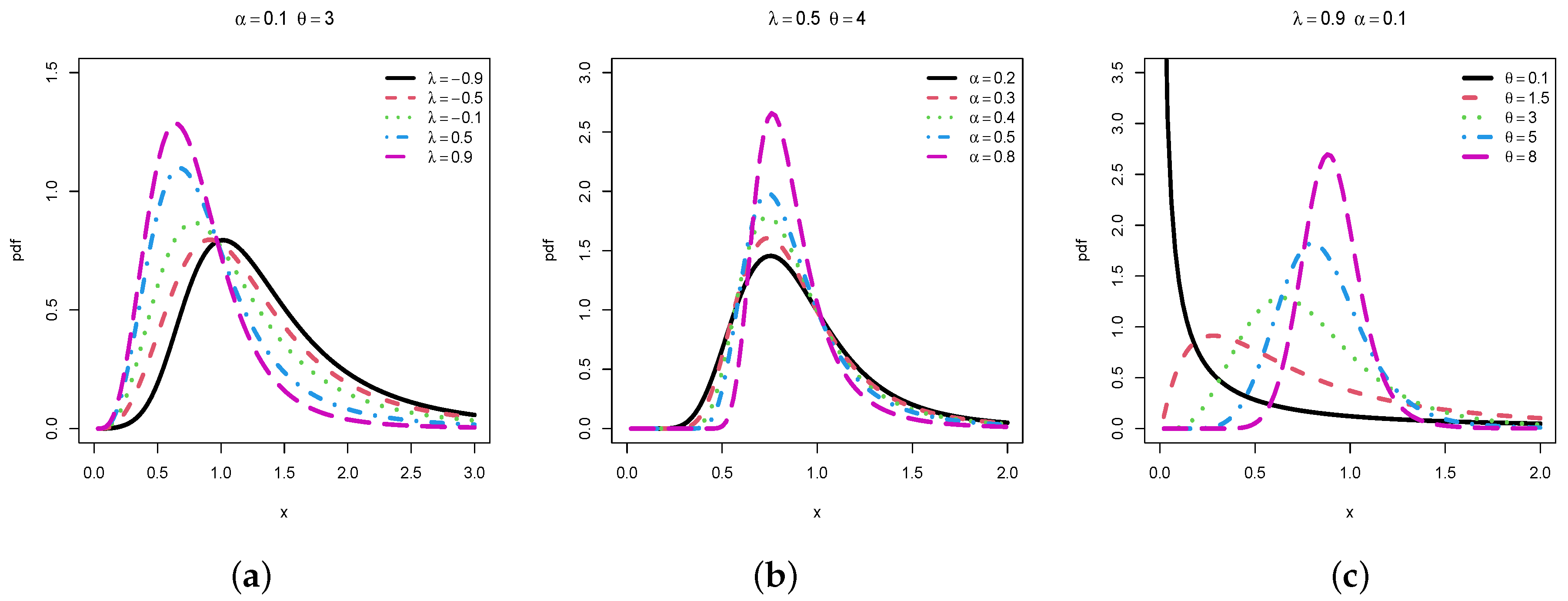
All the theory developed in the sections above can be applied to the TMLL distribution. Here, we go straight to the point by performing a graphical study on the critical points and possible shapes of $f(x;\mathsf{\Omega })$ and $h(x;\mathsf{\Omega })$. First, Figure 1 shows the possible shapes of $f(x;\mathsf{\Omega })$ by varying only one of the parameters.

Figure 1. Curves of the pdf of the TMLL distribution by varying (a) $\lambda$, (b) $\alpha$ and (c) $\theta$.

In particular, we see that the TMLL distribution is mainly unimodal, and is versatile in skewness and kurtosis. For the considered values of the parameters, $\lambda$ mainly affects the degree of right-skewness, $\alpha$ mainly impacts the peak of the pdf; we observe that increasing $\alpha$ clearly inceases this peak, and $\theta$ shows a strong influence on the mode and the overall curvature, making the pdf possibly decreasing. The decreasing property is mainly observed for the small values of $\theta$.

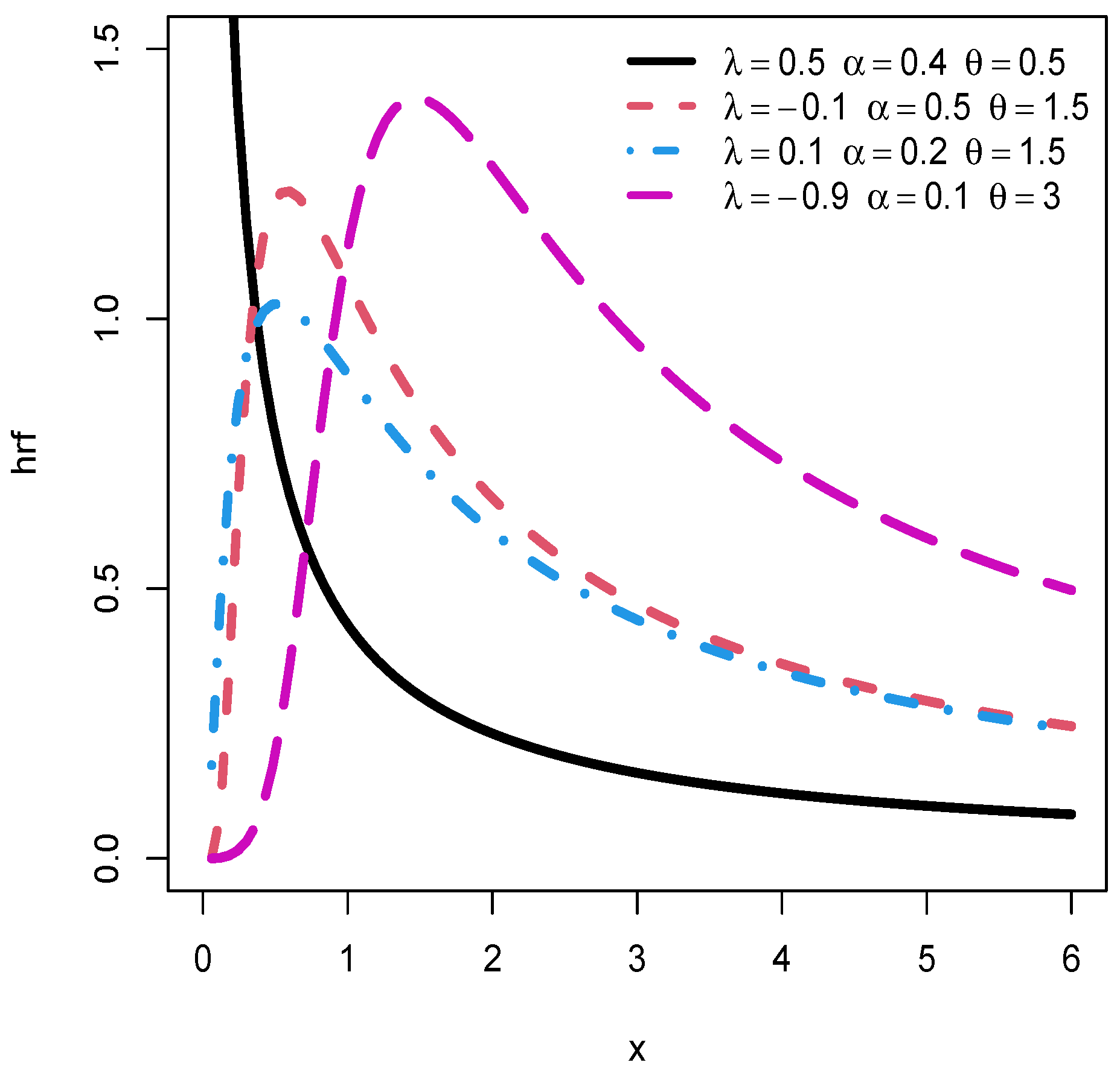
Figure 2 is about the possible shapes of $h(x;\mathsf{\Omega })$ for four sets of parameters.

Figure 2. Curves of the hrf of the TMLL distribution for some values of $\lambda$, $\alpha$ and $\theta$.

We observe in Figure 2 that the hrf has decreasing, and increasing-decreasing shapes when a maximum is observed. These characteristics are desirable for the modelling in diverse lifetime phenomena, as discussed in [25].

4.2. Parametric Estimation

The parameters of the TMLL model can be estimated through the ML approach, as developed in Section 3.3. In order to check the convergence of the obtained estimates, we perform a simulation study with samples of varying sizes. We thus examine the numerical properties of the corresponding ML estimates, mean square errors (MSEs), and average lengths (ALs) and coverage probabilities (CPs) of CIs at a certain fixed level.

More precisely, we generate $N=5000$ random samples of n values from the TMLL distribution defined with some (known) values of the parameters through the inverse transform sampling method. Then, we determine the average ML estimates, MSEs and average ALs of CIs at the levels $90\%$, and $95\%$. We do that for chosen increasing values of n, that is $n=20$, 50, 100, 200, 300, and 1000, in order to see if (i) the ML estimates tend to the true values of the parameters, (ii) the MSEs decrease to 0, (iii) the ALs become smaller and (iv) the CPs tend to the expected values, i.e., $0.90$ or $0.95$, depending on the considered level. The obtained results are put in Table 1, Table 2 and Table 3.

Table 1. ML estimates, MSEs, ${\mathrm{B}}_{-}$, ${\mathrm{B}}_{+}$, ALs and CPs under the following configuration: $\alpha =0.2$, $\lambda =-0.2$, and $\theta =1.2$.

n	par	MLE	MSE	Level 90%				Level 95%
				${\mathbf{B}}_{-}$	${\mathbf{B}}_{+}$	AL	CP	${\mathbf{B}}_{-}$	${\mathbf{B}}_{+}$	AL	CP
20	$\alpha$	0.4360	0.2005	−0.5415	1.4134	1.9548	0.5921	−0.7286	1.6006	2.3292	0.6208
	$\lambda$	−0.4365	0.2050	−2.3971	1.9241	4.3212	0.6242	−2.8108	2.3378	5.1486	0.6310
	$\theta$	0.9415	0.1400	0.0365	1.8465	1.8100	0.7012	−0.1368	2.0198	2.1567	0.7112
50	$\alpha$	0.3404	0.1773	0.1178	0.9630	0.8453	0.6451	0.0369	1.0440	1.0071	0.6523
	$\lambda$	−0.3804	0.1419	−0.7885	0.0276	0.8160	0.6551	−0.8666	0.1057	0.9723	0.6702
	$\theta$	0.9694	0.1182	0.6082	1.2707	0.6625	0.7332	0.5448	1.3341	0.7894	0.7382
100	$\alpha$	0.1628	0.1420	−0.2318	0.3573	0.5891	0.6822	−0.2882	0.4137	0.7019	0.7015
	$\lambda$	−0.1720	0.1136	−0.3389	0.1949	0.5338	0.6998	−0.3900	0.2460	0.6360	0.7124
	$\theta$	1.0131	0.0411	0.9900	1.4363	0.4463	0.7401	0.9473	1.4790	0.5317	0.7726
200	$\alpha$	0.1629	0.1134	−0.0558	0.3816	0.4374	0.8013	−0.0977	0.4235	0.5211	0.8459
	$\lambda$	−0.2285	0.0739	−0.4217	0.0048	0.4264	0.8533	−0.4625	0.0456	0.5081	0.8624
	$\theta$	1.1433	0.0420	0.9701	1.3166	0.3466	0.8212	0.9369	1.3498	0.4129	0.8907
300	$\alpha$	0.1884	0.0477	0.1272	0.4696	0.3424	0.8665	0.0944	0.5024	0.4079	0.9004
	$\lambda$	−0.2073	0.0552	−0.4626	−0.0519	0.4106	0.8727	−0.5019	−0.0126	0.4893	0.9148
	$\theta$	1.1714	0.0334	0.9778	1.2851	0.3073	0.8704	0.9483	1.3145	0.3662	0.9065
1000	$\alpha$	0.1910	0.0429	0.1649	0.4171	0.2522	0.8934	0.1408	0.4413	0.3005	0.9395
	$\lambda$	−0.2035	0.0402	−0.4435	−0.1234	0.3201	0.8901	−0.4742	−0.0928	0.3814	0.9413
	$\theta$	1.1875	0.0277	1.0032	1.2319	0.2287	0.8941	0.9813	1.2538	0.2725	0.9420

Table 2. ML estimates, MSEs, ${\mathrm{B}}_{-}$, ${\mathrm{B}}_{+}$, ALs and CPs under the following configuration: $\alpha =0.05$, $\lambda =0.1$, and $\theta =1.2$.

n	par	MLE	MSE	Level 90%				Level 95%
				${\mathbf{B}}_{-}$	${\mathbf{B}}_{+}$	AL	CP	${\mathbf{B}}_{-}$	${\mathbf{B}}_{+}$	AL	CP
20	$\alpha$	0.1146	0.4112	−0.7105	0.8197	1.5301	0.7008	−0.8570	0.9662	1.8231	0.7154
	$\lambda$	−0.1034	0.2164	−0.6624	0.4556	1.1180	0.6542	−0.7694	0.5626	1.3321	0.6712
	$\theta$	1.2189	0.2340	0.7031	1.7347	1.0316	0.6831	0.6044	1.8335	1.2291	0.7020
50	$\alpha$	0.0122	0.2647	−0.0305	0.7554	0.7859	0.7198	−0.1057	0.8306	0.9364	0.7352
	$\lambda$	−0.2200	0.1948	−0.5348	0.0948	0.6296	0.6928	−0.5951	0.1551	0.7502	0.7221
	$\theta$	1.1291	0.1969	0.8248	1.4334	0.6086	0.7353	0.7665	1.4917	0.7252	0.7519
100	$\alpha$	0.0148	0.0604	−0.2415	0.2712	0.5127	0.7402	−0.2906	0.3203	0.6109	0.7649
	$\lambda$	0.1411	0.0440	−0.1570	0.4192	0.5763	0.7550	−0.2122	0.4744	0.6866	0.7711
	$\theta$	1.1448	0.0132	0.9439	1.3456	0.4017	0.7841	0.9055	1.3841	0.4786	0.8005
200	$\alpha$	0.0328	0.0483	−0.0172	0.2887	0.3059	0.8436	−0.0465	0.3180	0.3645	0.8627
	$\lambda$	0.0763	0.0688	−0.1359	0.2884	0.4243	0.8532	−0.1765	0.3290	0.5055	0.8658
	$\theta$	1.1589	0.0256	0.9808	1.2570	0.2762	0.8401	0.9544	1.2834	0.3290	0.8749
300	$\alpha$	0.0695	0.0024	−0.0549	0.1939	0.2489	0.8673	−0.0788	0.2178	0.2965	0.9064
	$\lambda$	0.0871	0.0088	−0.1021	0.2764	0.3784	0.8792	−0.1383	0.3126	0.4509	0.9064
	$\theta$	1.1682	0.0026	1.0794	1.3171	0.2377	0.8798	1.0566	1.3398	0.2832	0.9121
1000	$\alpha$	0.0805	0.0010	0.0078	0.2132	0.2054	0.8902	−0.0119	0.2328	0.2447	0.9442
	$\lambda$	0.0915	0.0011	−0.1288	0.1719	0.3008	0.8890	−0.1576	0.2007	0.3583	0.9381
	$\theta$	1.1920	0.0014	1.0681	1.2558	0.1878	0.8956	1.0501	1.2738	0.2237	0.9425

Table 3. ML estimates, MSEs, ${\mathrm{B}}_{-}$, ${\mathrm{B}}_{+}$, ALs and CPs under the following configuration: $\alpha =0.6$, $\lambda =-0.5$, and $\theta =0.9$.

n	par	MLE	MSE	Level 90%				Level 95%
				${\mathbf{B}}_{-}$	${\mathbf{B}}_{+}$	AL	CP	${\mathbf{B}}_{-}$	${\mathbf{B}}_{+}$	AL	CP
20	$\alpha$	0.2021	1.3511	−1.7312	2.1354	3.8666	0.6104	−2.1014	2.5056	4.6070	0.6451
	$\lambda$	0.0356	0.9516	−3.4211	3.4924	6.9135	0.5923	−4.0831	4.1543	8.2374	0.6048
	$\theta$	1.2562	1.3025	0.6648	1.8475	1.1827	0.6826	0.5516	1.9607	1.4092	0.7025
50	$\alpha$	0.4018	0.6149	−0.1362	0.9997	1.1359	0.6531	−0.2449	1.1085	1.3534	0.6821
	$\lambda$	−0.2286	0.8551	−1.2861	0.4288	1.7149	0.6223	−1.4503	0.5930	2.0433	0.6473
	$\theta$	1.0176	0.0212	0.4496	1.4256	0.9760	0.7055	0.3561	1.5190	1.1629	0.7224
100	$\alpha$	0.4209	0.5360	0.1773	0.6645	0.4872	0.7270	0.1307	0.7111	0.5804	0.7305
	$\lambda$	−0.3615	0.6607	−0.5020	−0.2209	0.2812	0.6969	−0.5290	−0.1939	0.3350	0.7095
	$\theta$	1.0351	0.6346	0.8569	1.2134	0.3564	0.7532	0.8228	1.2475	0.4247	0.7610
200	$\alpha$	0.5365	0.4155	0.3647	0.7082	0.3436	0.8316	0.3318	0.7411	0.4094	0.8454
	$\lambda$	−0.3646	0.4301	−0.4944	−0.2347	0.2597	0.8253	−0.5193	−0.2099	0.3094	0.8611
	$\theta$	0.9970	0.4514	0.8556	1.1383	0.2828	0.8570	0.8285	1.1654	0.3369	0.8911
300	$\alpha$	0.6506	0.3953	0.5141	0.7871	0.2730	0.8753	0.4880	0.8133	0.3253	0.9141
	$\lambda$	−0.5095	0.4003	−0.5916	−0.4274	0.1642	0.8892	−0.6073	−0.4116	0.1957	0.9274
	$\theta$	0.9148	0.3868	0.8086	1.0209	0.2123	0.8685	0.7883	1.0412	0.2530	0.9207
1000	$\alpha$	0.6105	0.3308	0.4987	0.7224	0.2237	0.8944	0.4773	0.7438	0.2665	0.9453
	$\lambda$	−0.5053	0.2671	−0.5570	−0.4537	0.1033	0.8978	−0.5668	−0.4438	0.1230	0.9485
	$\theta$	0.9058	0.3095	0.8252	0.9863	0.1612	0.8901	0.8097	1.0018	0.1920	0.9422

From Table 1, Table 2 and Table 3, it is clear that the ML estimates converge to the corresponding values of the parameters. Furthermore, when n increases, the MSEs decrease to 0, the ALs becomes smaller and the CPs tend to the considered level value. This motivates us to use the ML approach in estimation of the parameters of the TMLL model.

4.3. Applications

We now apply the TMLL model, along with the ML approach, to show its adequacy with environmental and survival data. The two considered data sets are described below.

Data set I: the first data set is obtained from [32]. It contains 30 successive values of March precipitation (in inches) in Minneapolis. The data are as follows:

0.77; 1.74; 0.81; 1.20; 1.95; 1.20; 0.47; 1.43; 3.37; 2.20; 3.00; 3.09; 1.51; 2.10; 0.52; 1.62; 1.31; 0.32; 0.59; 0.81; 2.81; 1.87; 1.18; 1.35; 4.75; 2.48; 0.96; 1.89; 0.90; 2.05.

Data set II: the second data set is obtained from [33]. It represents the survival times (in days) of 72 guinea pigs infected with mortal bacteria (tubercle bacilli). The data are as follows: 0.10; 0.33; 0.44; 0.56; 0.59; 0.72; 0.74; 0.77; 0.92; 0.93; 0.96; 1.00; 1.00; 1.02; 1.05; 1.07; 1.07; 1.08; 1.08; 1.08; 1.09; 1.12; 1.13; 1.15; 1.16; 1.20; 1.21; 1.22; 1.22; 1.24; 1.30; 1.34; 1.36; 1.39; 1.44; 1.46; 1.53; 1.59; 1.60; 1.63; 1.63; 1.68; 1.71; 1.72; 1.76; 1.83; 1.95; 1.96; 1.97; 2.02; 2.13; 2.15; 2.16; 2.22; 2.30; 2.31; 2.40; 2.45; 2.51; 2.53; 2.54; 2.54; 2.78; 2.93; 3.27; 3.42; 3.47; 3.61; 4.02; 4.32; 4.58; 5.55.

Table 4 presents the descriptive statistics of these data sets.

Table 4. Statistical description of the two data sets.

Data Set	n	Mean	Median	Standard Deviation	Skewness	Excess of Kurtosis
I	30	1.68	1.47	1.00	1.03	0.93
II	72	1.77	1.50	1.04	1.31	1.85

It is clear that the data sets mainly differ in their kurtosis nature. Now, we aim to compare the fit power of the TMLL model with those of the following famous models:

• Burr XII (BXIII) with cdf defined by

  $$\begin{array}{c}\hfill F(x;\alpha ,\beta )=1-{(1+x^{\alpha })}^{-\beta },x>0,\end{array}$$

  where $\alpha >0$ and $\beta >0$.
• Beta log-logistic (BLL) (see [34]) with cdf specified by

  $$\begin{array}{c}\hfill F(x;\alpha ,\theta ,\lambda )=\frac{1}{B(\lambda ,\alpha )}{\int }_0^{1-{(1+x^{\theta })}^{-1}}{t}^{\lambda -1}{(1-t)}^{\alpha -1}dt,x>0,\end{array}$$

  where $B(\lambda ,\alpha )$ denotes the classical beta function, $\alpha >0$, $\theta >0$ and $\lambda >0$.
• Muth (M) model with cdf given as (1) with parameter $\alpha >0$.

As a first step, we determine the ML estimates of all the parameters of the models in Table 5 and Table 6, for data sets I and II, respectively.

Table 5. ML estimates with their corresponding standard errors for data set I.

Model	$\mathit{\lambda }$	$\mathit{\alpha }$	$\mathit{\theta }$	$\mathit{\beta }$
TMLL	−0.9716	−0.1834	2.6321	-
	(0.6601)	(0.5570)	(0.4147)	-
BXII	-	3.2554	-	0.5769
	-	(0.6454)	-	(0.1371)
BLL	37.4470	32.9595	0.3851	-
	(6.2045)	(7.6753)	(0.7332)	-
M	-	0.1846	-	-
	-	(0.0906)	-	-

Table 6. ML estimates with their corresponding standard errors for data set II.

Model	$\mathit{\lambda }$	$\mathit{\alpha }$	$\mathit{\theta }$	$\mathit{\beta }$
TMLL	−0.7209	−0.5432	2.8084	-
	(0.2989)	(0.2616)	(0.2220)	-
BXII	-	3.8132	-	0.4782
	-	(0.5440)	-	(0.0792)
BLL	4.2308	2.6652	1.3490	-
	(5.4761)	(4.2066)	(1.1359)	-
M	-	0.1492	-	-
	-	(0.0555)	-	-

From these tables, concerning the TMLL model, we see that the parameter $\lambda$ is estimated “relatively far” to 0, motivating the use of the transmuted scheme. Furthermore, the parameter $\alpha$ is negatively estimated, attesting the importance of the new remarks formulated in Section 2.1.

We now compare the models through the following well-established criteria: Akaike and Bayesian information criteria (AIC and BIC), Cramer–von Mises (W), and Anderson–Darling (A). Roughly speaking, the smaller the values of these criteria, the better the model is in the fit of the data. The R software is used, along with the package AdequacyModel by [28]. Table 7 and Table 8 collect the obtained results.

Table 7. Values of statistical criteria for models comparison for data set I.

Model	AIC	BIC	W	A
TMLL	84.2478	88.4514	0.0357	0.2313
BXII	85.7804	88.5827	0.0696	0.4299
BLL	85.0294	89.2330	0.0377	0.2427
M	99.4455	100.8467	0.2470	0.8927

Table 8. Values of statistical criteria for models comparison for data set II.

Model	AIC	BIC	W	A
TMLL	191.9918	198.8218	0.0491	0.3234
BXII	200.8386	205.3920	0.1193	0.8993
BLL	200.3750	207.2050	0.0964	0.7178
M	251.0743	253.3510	0.1651	0.9750

Since it has the smallest values of AIC, BIC and A the TMLL model is the best among them all, for the two data sets. In particular, it outperforms the BLL model, and thus represents a better extension of the log-logistic model for the considered data sets.

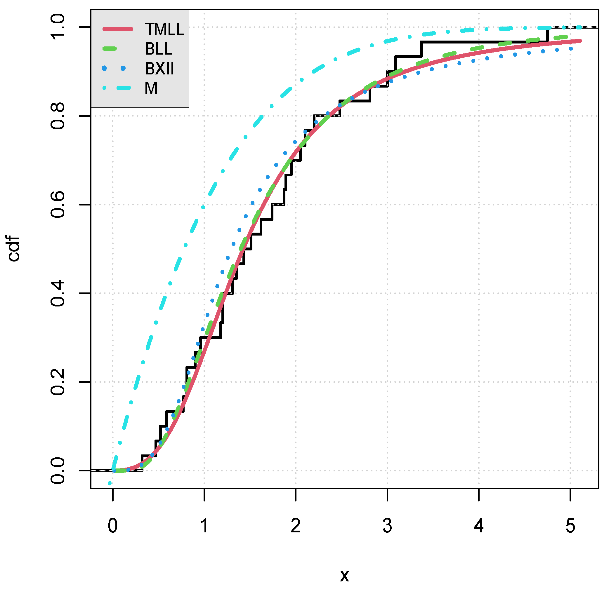
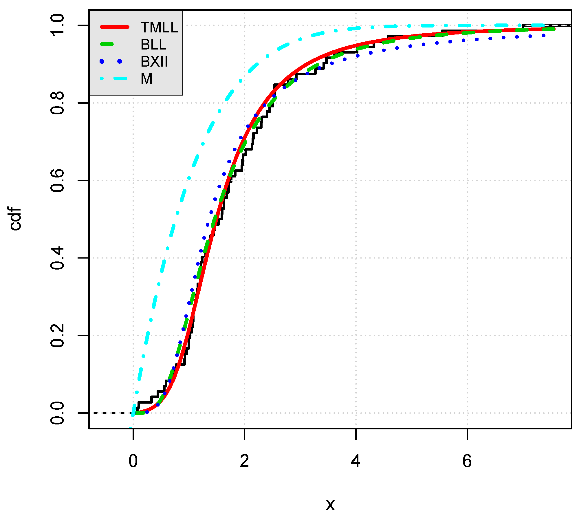
We now illustrate graphically the adequacy of the model by plotting the following objects:

• The curve of the estimated cdf of the TMLL model, i.e., $F(x;\tilde{\mathsf{\Omega }})$, as well as the curves of the estimated cdfs of the other models over the curve of the empirical cdf for data sets I and II in Figure 3 and Figure 4, respectively.
  

  Figure 3. Curves of the estimated cdfs of the considered models over the empirical cdf for data set I.
  

  Figure 4. Curves of the estimated cdfs of the considered models over the empirical cdf for data set II.
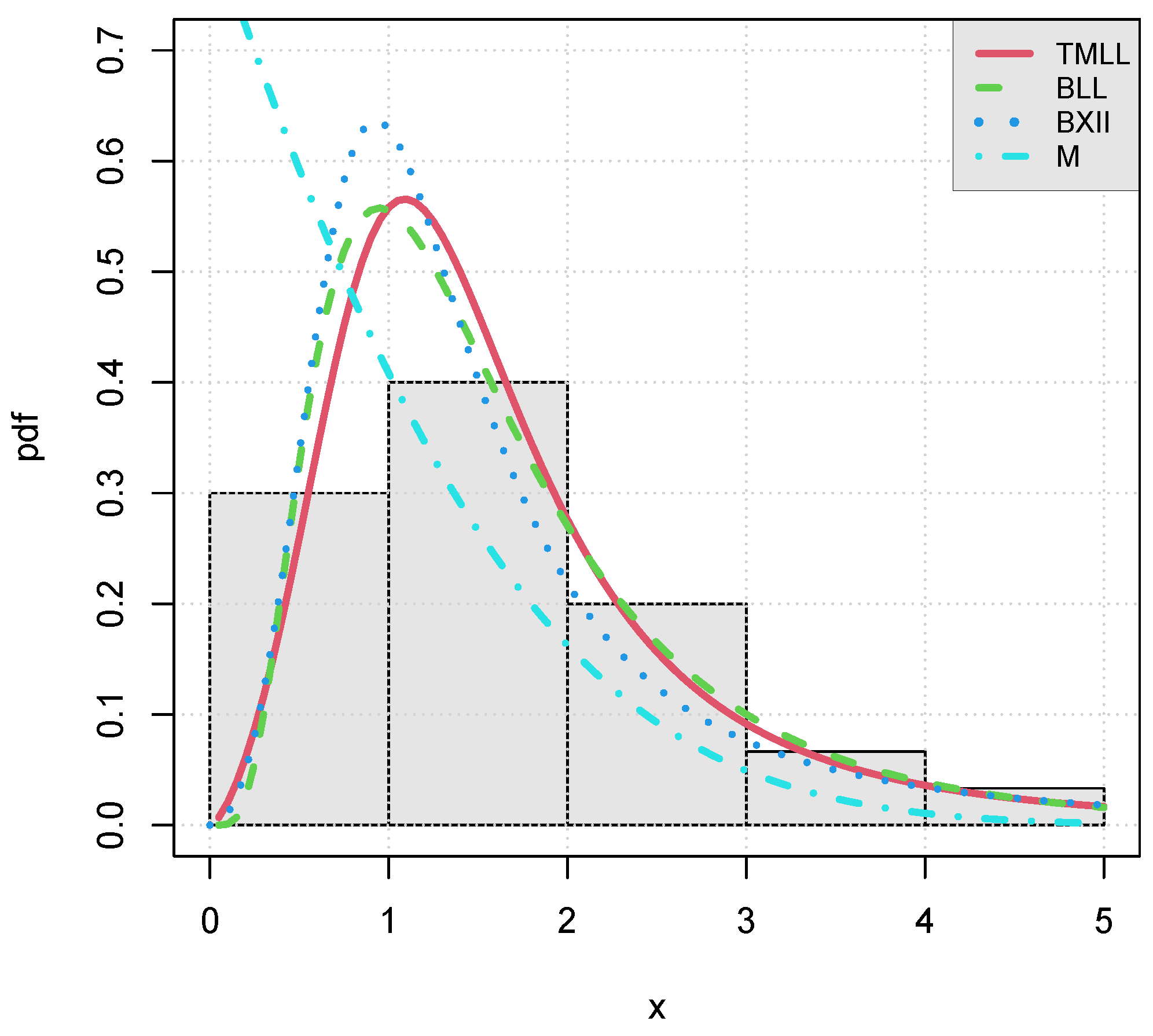
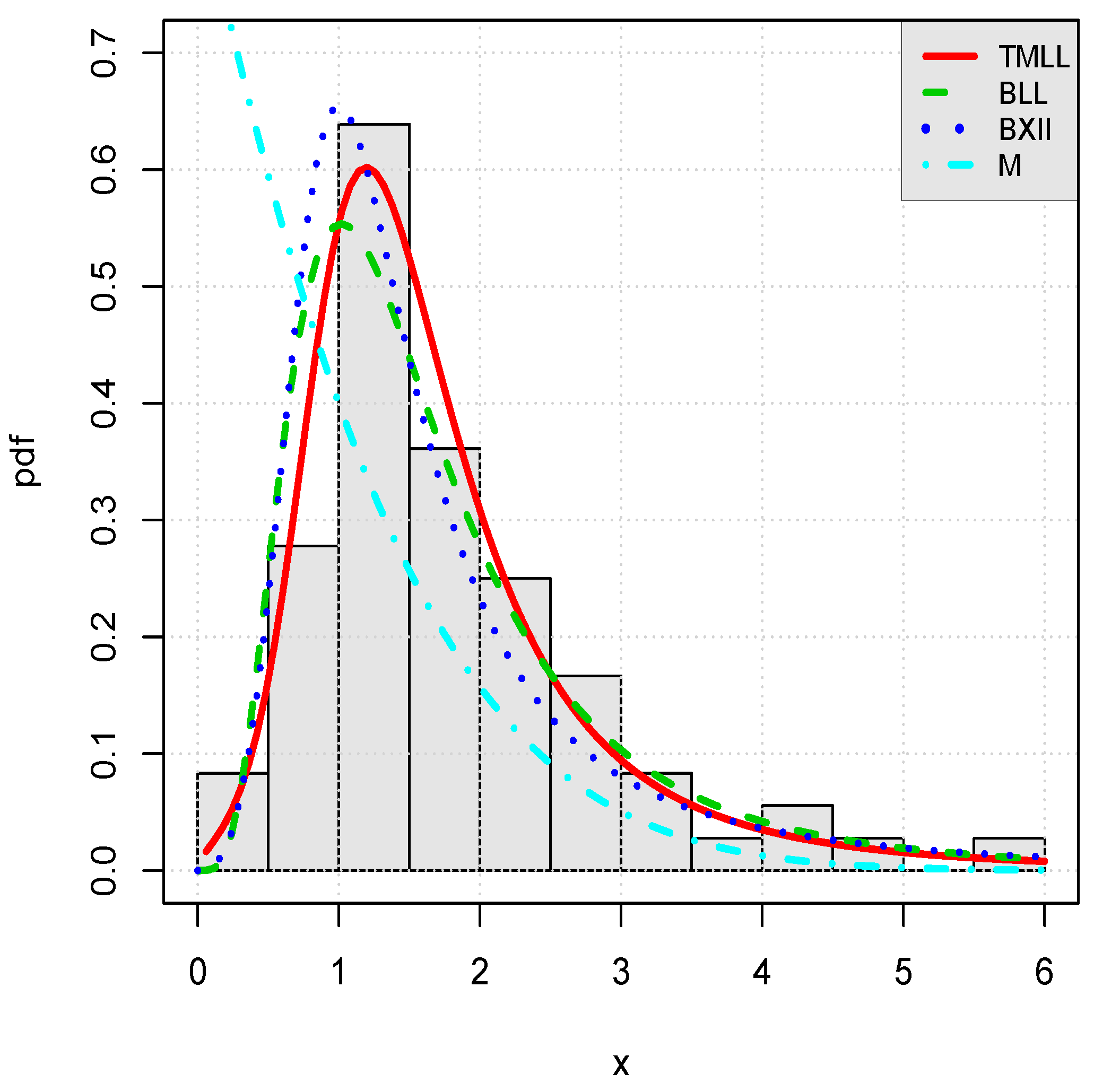
• The curve of the estimated pdf of the TMLL model, i.e., $f(x;\tilde{\mathsf{\Omega }})$, as well as the curves of the estimated pdfs of the other models, all over the histogram for data sets I and II in Figure 5 and Figure 6, respectively.
  

  Figure 5. Curves of the estimated pdfs of the considered models over the histogram for data set I.
  

  Figure 6. Curves of the estimated pdfs of the considered models over the histogram for data set II.

Visually, the fits of the TMLL model are quite satisfying, as anticipated.

5. Concluding Remarks and Perspectives

This study contributes to the development of the M-G class by showing new facts, and by proposing a motivated extending class, called the transmuted Muth generated class of distributions. We derive several of its probabilistic and analytical properties, including the expressions of the pdf and hrf, discussions on their critical points, expression of the qf, series expansions for various moments and theory on the parametric estimation of the parameters. Then, a focus is put on the special distribution of the TM-G class, called the transmuted Muth log-logistic distribution. We show that this distribution is flexible enough to fit various symmetrical or right-skewed data. Combined with the maximum likelihood approach, the fit behavior of the model is discussed through the analysis of two real data sets. The adequacy of the new model is quite satisfactory, beating the one of the famous beta log-logistic model. As further developments, one can investigate other special distributions of the TM-G class, as those having support in $(0,1)$ or $\mathbb{R}$, finding applications in diverse regression models. The regression aspect, however, needs further investigations in the future.

References

- Muth, J.E. Reliability models with positive memory derived from the mean residual life function. In The Theory and Applications of Reliability; Tsokos, C.P., Shimi, I., Eds.; Academic Press: New York, NY, USA, 1977; Volume 2, pp. 401–435. [Google Scholar]
- Jodrá, P.; Jiménez-Gamero, M.D.; Alba-Fernández, M.V. On the Muth distribution. Math. Model. Anal. 2015, 20, 291–310. [Google Scholar] [CrossRef]
- Leemis, L.M.; McQueston, J.T. Univariate distribution relationships. Am. Stat. 2008, 62, 45–53. [Google Scholar] [CrossRef]
- Jodrá, P.; Gómez, H.W.; Jiménez-Gamero, M.D.; Alba-Fernández, M.V. The power Muth distribution. Math. Model. Anal. 2017, 22, 186–201. [Google Scholar] [CrossRef]
- Almarashi, A.M.; Elgarhy, M. A new Muth generated family of distributions with applications. J. Nonlinear Sci. Appl. 2018, 11, 1171–1184. [Google Scholar] [CrossRef]
- Alzaatreh, A.; Lee, C.; Famoye, F. A new method for generating families of continuous distributions. Metron 2013, 71, 63–79. [Google Scholar] [CrossRef]
- Abouelmagd, T.H.M.; Al-mualim, S.; Elgarhy, M.; Afify, A.Z.; Ahmad, M. Properties of the four-parameter Weibull distribution and its applications. Pak. J. Stat. 2017, 33, 449–466. [Google Scholar]
- Lee, C.; Famoye, F.; Olumolade, O. Beta-Weibull distribution: Some properties and applications to censored data. J. Mod. Appl. Stat. Meth. 2007, 6, 173–186. [Google Scholar] [CrossRef]
- Cordeiro, G.M.; Hashimoto, E.M.; Ortega, E.M.M. The McDonald Weibull model. Statistics 2014, 48, 256–278. [Google Scholar] [CrossRef]
- Mudholkar, G.S.; Srivastava, D.K. Exponentiated Weibull family for analysing bathtub failure rate data. IEEE Trans. Reliab. 1993, 42, 299–302. [Google Scholar] [CrossRef]
- Al-babtain, A.; Elbatal, I.; Yousof, H.M. A new flexible three-parameter model: Properties, Clayton copula, and modeling real data. Symmetry 2020, 12, 440. [Google Scholar] [CrossRef]
- Almarashi, A.M.; Elgarhy, M.; Jamal, F.; Chesneau, C. The exponentiated truncated inverse Weibull generated family of distributions with applications. Symmetry 2020, 12, 650. [Google Scholar] [CrossRef]
- Bantan, R.A.R.; Jamal, F.; Chesneau, C.; Elgarhy, M. Type II Power Topp-Leone generated family of distributions with statistical inference and applications. Symmetry 2020, 12, 75. [Google Scholar] [CrossRef]
- ZeinEldin, R.A.; Jamal, F.; Chesneau, C.; Elgarhy, M. Type II Topp-Leone inverted Kumaraswamy distribution with statistical inference and applications. Symmetry 2019, 11, 1459. [Google Scholar] [CrossRef]
- Shaw, W.T.; Buckley, I.R. The alchemy of probability distributions: Beyond Gram-Charlier expansions, and a skew-kurtotic-normal distribution from a rank transmutation map. arXiv 2009, arXiv:0901.0434. [Google Scholar]
- Gupta, R.D.; Kundu, D. Exponentiated exponential family: An alternative to Gamma and Weibull distributions. Biom. J. 2001, 43, 117–130. [Google Scholar] [CrossRef]
- Sangsanit, Y.; Bodhisuwan, W. The Topp-Leone generator of distributions: Properties and inferences. Songklanakarin J. Sci. Technol. 2016, 38, 537–548. [Google Scholar]
- Alizadeh, M.; Rasekhi, M.; Yousof, H.M.; Hamedani, G.G. The transmuted Weibull-G family of distributions. Hacet. J. Math. Stat. 2018, 47, 1671–1689. [Google Scholar] [CrossRef]
- Badr, M.A.; Elbatal, I.; Jamal, F.; Chesneau, C.; Elgarhy, M. The transmuted odd Fréchet-G family of distributions: Theory and applications. Mathematics 2020, 8, 958. [Google Scholar] [CrossRef]
- Nofal, Z.M.; Afify, A.Z.; Yousof, H.M.; Cordeiro, G.M. The generalized transmuted-G family of distributions. Commun. Stat. Theory Methods 2017, 46, 4119–4136. [Google Scholar] [CrossRef]
- Reyad, H.; Jamal, F.; Othman, S.; Hamedani, G.G. The transmuted Gompertz-G family of distributions: Properties and applications. Tbil. Math. J. 2018, 11, 47–67. [Google Scholar] [CrossRef]
- Reyad, H.; Othman, S.; Ul Haq, M.A. The transmuted generalized odd generalized exponential-G family of distributions: Theory and applications. J. Data Sci. 2019, 17, 279–300. [Google Scholar]
- Yousof, H.M.; Afify, A.Z.; Alizadeh, M.; Butt, N.S.; Hamedani, G.G.; Ali, M.M. The transmuted exponentiated generalized-G family of distributions. Pak. J. Stat. Oper. Res. 2015, 11, 441–464. [Google Scholar] [CrossRef]
- Haq, M.A.; Elgarhy, M. The odd Fréchet-G family of probability distributions. J. Stat. Appl. Probab. 2018, 7, 189–203. [Google Scholar] [CrossRef]
- Aarset, M.V. How to identify bathtub hazard rate. IEEE Trans. Reliab. 1987, 36, 106–108. [Google Scholar] [CrossRef]
- Cordeiro, G.M.; Silva, R.B.; Nascimento, A.D.C. Recent Advances in Lifetime and Reliability Models; Bentham Sciences Publishers: Sharjah, UAE, 2020. [Google Scholar]
- Casella, G.; Berger, R.L. Statistical Inference; Brooks/Cole Publishing Company: Bel Air, CA, USA, 1990. [Google Scholar]
- Marinho, P.R.D.; Silva, R.B.; Bourguignon, M.; Cordeiro, G.M.; Nadarajah, S. AdequacyModel: An R package for probability distributions and general purpose optimization. PLoS ONE 2019, 14, e0221487. [Google Scholar] [CrossRef] [PubMed]
- Bennett, S. Log-logistic regression models for survival data. Appl. Stat. 1983, 32, 165–171. [Google Scholar] [CrossRef]
- Shoukri, M.M.; Mian, I.U.M.; Tracy, D.S. Sampling properties of estimators of the log-logistic distribution with application to Canadian precipitation data. Can. J. Stat. 1988, 16, 223–236. [Google Scholar] [CrossRef]
- Ashkar, F.; Mahdi, S. Fitting the log-logistic distribution by generalized moments. J. Hydrol. 2006, 328, 694–703. [Google Scholar] [CrossRef]
- Hinkley, D. On quick choice of power transformations. J. R. Stat. Soc. Ser. Appl. Stat. 1977, 26, 67–69. [Google Scholar] [CrossRef]
- Bjerkedal, T. Acquisition of resistance in guinea pigs infected with different doses of virulent tubercle bacilli. Am. J. Hyg. 1960, 72, 130–148. [Google Scholar]
- Lemonte, A.J. The beta log-logistic distribution. Braz. J. Probab. Stat. 2014, 28, 313–332. [Google Scholar] [CrossRef]
Publisher’s Note: MDPI stays neutral with regard to jurisdictional claims in published maps and institutional affiliations. |
© 2020 by the authors. Licensee MDPI, Basel, Switzerland. This article is an open access article distributed under the terms and conditions of the Creative Commons Attribution (CC BY) license (http://creativecommons.org/licenses/by/4.0/).