Article

Ergodic Tendencies in Sub-Systems Coupled to Finite Reservoirs—Classical and Quantal

Physics Department, Ariel University, Ariel 40700, Israel
Symmetry 2020, 12(10), 1642; https://doi.org/10.3390/sym12101642
Submission received: 2 September 2020 / Revised: 23 September 2020 / Accepted: 24 September 2020 / Published: 6 October 2020
(This article belongs to the Section Physics)

Abstract

:
Whereas ergodic theories relate to limiting cases of infinite thermal reservoirs and infinitely long times, some ergodicity tendencies may appear also for finite reservoirs and time durations. These tendencies are here explored and found to exist, but only for extremely long times and very soft ergodic criteria. “Weak ergodicity breaking” is obviated by a judicious time-weighting, as found in a previous work [Found. Phys. (2015) 45: 673–690]. The treatment is based on an N-oscillator (classical) and an N-spin (quantal) model. The showing of ergodicity is facilitated by pictorial presentations.

1. Introduction

In a broadly phrased description, ergodic theorems equate time and ensemble averages [1,2,3,4,5,6], and take various forms both in the precise definition of the term “equate” (which is usually done in the senses of Set Theory, for example, References [7,8]) and of the variety of items whose averages are considered. As regards the former, physical applications of ergodicity (as in References [9,10]) typically steer clear of the niceties (e.g., the qualification of “almost all”) of set-theoretical precision [11,12], as is being done here. The varieties of theorems are features of both developments in the course of times and at a particular time of the subject matters which are at interest. Historically, Poincaré [13] is regarded, through his recurrence theorem, as the progenitor of Ergodic Theory, which had led to Boltzmann’s Statistical Mechanics and Entropy concept for the dynamical theory of gases [14]. At the basis of ergodic theory as applied to dynamical systems is what is termed “the invariant measure”, whose meaning is roughly the uniformity of the statistical weight of the system over states that it potentially partakes of. (It is this weight that enters logarithmically the entropy concept of Boltzmann, taught in every elementary course on Statistical Mechanics. Related to this is the “Metrical Decomposability” of von Neumann [15]). Microcanonical ensembles, that is, those whose manifold sub-systems have a fixed total energy, possess this property and ergodicity in its multiplicity of set-theoretical senses referred in its primary applicability to these. (In truth, the potential applicabilities of ergodicity are extremely broad, encompassing beyond the exact sciences also biology, sociology, medicine and humanities, for example, Reference [16]).
Constituent parts, “sub-systems” of systems forming a microcanonical ensemble do not possess “the invariant measure” property (as elucidated in further detail later on in this article), and general theories do not appear to hold for these. Thence, there is some value in studying some particular models (and, at it, some simple ones), with a view of gaining some knowledge of ergodic behaviors or otherwise, in these systems, where they are not mandated. Previous work [17,18] went in this direction. The present article amplifies the knowledge by including classical, as well as quantum systems (in Section 2 and Section 3, respectively). The net conclusion arising from our (mainly numerical) results is that ergodic behavior is a property also of systems lacking “invariant measures”, but only approximately so and with a critical amendment in the process of time averaging, namely by the appropriate and non-uniform weighting of the time (t, here termed the “sojourn duration”) in the time integration.
A further deviation of the present work from the routine are the “finitenesses (!)” of the objects, this in contrast to the mainstream of ergodicity studies, which deal with systems of infinite size and duration ("the thermodynamic limit") and are capable to yield formal results.
Moreover, in the following investigation of the onset of ergodicity in finite and transient systems, of size ( N < ) and time durations ( t r < ), consideration will be given to another, somewhat imprecise term that enters the following, accepted formulation of ergodicity: “In the ergodic limit, the path trajectory approaches arbitrarily near to every point in phase space” [1]. This nearness concept had been given crucial importance early on by the Ehrenfests [19,20]. In what follows the term “near” will enter in a numerically precise and important way through the nearness parameter “ n p ”, which is the measure of the distance between a chosen phase-space point ( X , P for a single classical particle) and the corresponding value on the trajectory. “Nearness” enters our computations in the following way:
In the sequel we establish the number of times the trajectory approaches closely to a given point X , P in phase space. If this approach takes place to within values of “np” for both the coordinate and the momenta, then this is counted as a visit; if it fails to do so for either, then this approach is not counted as a visit. Typical values to achieve ergodic tendencies in our finite systems are found with np not falling below a 0.02 fraction of the characteristic values in X and P (which are of the same order, in our system of units). Thus, we find that below this value of “np” the number of approaches, or “visits” (here designated N V , for visiting numbers) take effectively random values for different points in phase space; only above this tolerance ( n p > 0.02 ) are the visiting numbers distributed in a regular way. The regularities are discussed in the text.
The term “visiting number” leads us to consideration for classical dynamics of an allied quantity, the “sojourn time” already mentioned, being the time that the trajectory spends in the vicinity (defined here through n p ) of the phase-space point. Cases when this quantity is in violation of ergodicity were named by Bouchaud [21] “weak ergodic breaking” (distinct from “strong ergodicity breaking”, for which N V is also not ergodic) and were intensively studied by Barkai and collaborators, for example, for anomalous diffusers temporarily residing in traps [22,23,24,25] and more recently in Reference [26]. In contrast to these, the dynamic, continuously moving system studied here in the classical section shows no signs of weakly breaking of ergodicity.

The Models

The objects of our treatment in the classical domain are coupled oscillators, Section 2 a subject which lies at the basis of lattice dynamics and has been extensively studied for one-to-three dimensional systems. Finite numbers of interacting oscillators belong in reality to the realm of infra-red molecular spectra.
In the quantum regime we treat N interacting 1 / 2 -spins, Section 3. (Notably, the quantum description in this section centering in the interacting spins is conceptually simpler than the classical one, in so much as the phase space is one dimensional, labelled with r by the series of discrete eigen-energy values, regarded as non-degenerate. A reduction in complexity, in terms of information contents, of a quantum description of a random process relative to a classical one was noted in Reference [27]. A further distinction is on the minimal grid size in coordinate-momentum phase space of quantal systems required by the uncertainty principle. Owing to the finite number of spins involved, cooperative effects like ferromagnetism are not applicable). Multiple interacting spin systems (chains)are currently at interest for their potentialapplications with a view to quantum metrology, as in Reference [28], and to information transfer, as in Reference [29]. Interacting systems having finite Hilbert state dimensions have also been theoretically researched for entanglement and other properties [30,31,32,33,34,35,36,37,38]. The more general topic of open systems was comprehensively treated in Reference [39].
On the experimental side, a quantum processor consisting of N = 8 coupled qubits and subject to time dependent interactions was studied with the view of achieving feasible quantum computing [40]. Finite number of interacting spins, (namely 15 spins forming a V 15 cluster) constituting a molecular magnet were the subject of Reference [41]: the nature of couplings in this system differs from the one considered in the present work, in that PI includes also Dzyaloshinsky-Moriya and hyperfine couplings. In contrast; our finite spin systems reach only up to only 9 spins, and for these numerical results are presented, they extrapolate nicely to the formal results for infinite, thermal reservoirs of Rechtman and Penrose [42].
To round up the picture, there remains the study of effects arising from the mutual interaction between the two entities, spins and oscillators. These have in the first instance entered the field as the Jaynes-Cummings model, subsequently they have later formed the subject of the broadly scoped review of Reference [43]. One also notes a further work framed in the adiabatic approximation in Reference [44]. From the present viewpoint of ergodicity in finite systems, a study of their properties is under consideration by us.
In a nutshell, the main conspicuous outcomes arising from the treatments in the present work, for either the classical or the quantum systems, are the extended establishment of ergodicity (beyond its basic theoretically warranted domain), but in a manner that depends quantitatively on some parameter values, and the requirement of unequal weighting of the time in taking the time averages.

2. Classical: N Oscillators

Here the time dependent displacement variable X 1 ( t ) of the sub-system is coupled to the displacement variables [ X 2 ( t ) , . . . . , X N ( t ) ] of the reservoir. A model is designed with the aim of tracing the (long time, but not infinitely long duration) movement of a privileged particle, this being part of a set of similar entities and calculating the frequency of its visiting each point in its (classical) phase space, represented by the position and momentum labels X , P . Such situation might exist for an isotopically labelled atom residing within a trapped molecule or a finite solid. Ergodicity minimally implies that all phase-space points in an active zone of the space are visited. Path trajectories and the 2D continuities of the space-phase being of different kinds (measures) of infinity, the term “visit” cannot mean exact coincidence and is defined here as events in which the trajectory approaches the X , P point within (with a “tolerance” of) a small value, here designated n p (for “nearness parameter”).
Equations of motion and solutions for the N particle coordinates and momenta [ X i ( t ) , P i ( t ) ; i = 1 , . . . , N ] being functions of time t, arise from a Hamiltonian
H N = K . E . + V ( { X i } )
in which the first, kinetic energy term K . E . is for N particles having masses that are (for simplicities’ sake) identical and of unit value, while the second, potential energy term is that of N bi-linearly interacting oscillators
V ( { X i } ) = 1 2 i , j X i M i j X j
with the elements of the dynamic matrix M i j chosen to have (again, for simplicity) unit values along the diagonal and rather arbitrarily (but with a view at some mnemonically simple and systematic rule of construction) the decimal fraction values at the r row and c column positions, of the form:
r < c : 0 . r c , r > c : 0 . c r , r = c : 1 ( r , c = 1 , . . . N ) ,
Thus, the dynamical matrix is symmetric.
Diagonalisation of the dynamic matrix, by means of the unitary transformation matrix A i n = A n i + , leads to the normal amplitude coordinates Q n = i = 1 , . . . , N A n i X i , ( n = 1 , . . . , N ) and their eigen-frequencies Ω n , such that solutions of the resulting equations of motion are of the form
Q n ( t ) = a n sin ( Ω n t + ϕ n )
with amplitudes a n and phases ϕ n whatever.

2.1. Ensemble Construction

It is important to recognize that to be physically meaningful, the construction must be done on initial values, at t = 0 , and on the physical amplitudes X i ( t = 0 ) , which are the physically accessible quantities, and not on the theoretical constructs Q n ( t = 0 ) . Historically, choices of ensembles have been frequently made, as in the works of Zwanzig, to those leading to a thermal equilibrium bath. Yet we are at liberty to define the constructed ensemble by any ensemble properties, and we impose on its construction the requirement that the ensemble averages of the amplitudes squared | X i ( 0 ) | 2 and of the momenta squared | P i ( 0 ) | 2 , are all fixed, precisely:
| < X i ( 0 ) 2 > | = 1 2 , | < P i ( 0 ) 2 > | = 1 2
for all i. To construct an ensemble satisfying these properties, we choose ensemble systems whose elements have random phases and, uniformly, unit strengths in the normal amplitudes of Equation (4), so that the expression for the i-th oscillator’s displacement has the form:
X i r ( t ) = n = 1 , . . . , N A i n cos ( Ω n t + ϕ n r )
(Meaning: a n in Equation (4) is unity and ϕ n r are random phase values). The proof for this assertion is given in Appendix B and is based on the following two properties of the transformation matrix A i n :
A n i A i m + = δ n m
A n i V i j A j m + = Ω n 2 δ n m
(the first being due to unitarity and the second being the defining choice of the transformation matrix).

2.2. The Visiting Number N V

We shall later return to the ensemble properties. Now we consider the dynamics of one particular, but hopefully representative system in the ensemble, defined by having one particular set of initial phase values. Out of the N local amplitudes X i ( t ) ( i = 1 , . . . , N ) in the system, we select one local oscillator X 1 ( t ) . This will be our privileged sub-system, with the remaining N 1 oscillators having now the role of a finite reservoir. Accordingly, the amplitude of the sub-system then takes the form of an almost periodic function. We thus rewrite Equation (6) to read
X 1 ( t ) = n = 1 , . . . , N A 1 n sin ( Ω n t + ( 2 π n ) / N )
with a specific choice of the phases, as written. Classical velocity of the sub-system particle is the time derivative of X 1 ( t ) , and due to our choice of unit masses for all, this is also the sub-system’s momentum P 1 ( t ) . Postulating that this amplitude is typical of those in other members in the ensemble, we next trace its temporal development in its phase-space.
Of interest is the number of times that the sub-system’s dynamical variables X 1 ( t ) , P 1 ( t ) approach jointly, in the course of the trajectory, points ( X , P ) on the phase-space plane, and this for all points thereon. The search for the number of such visits N V at each point is carried out as follows:
We partition the time t of progress along the trajectory into extremely small time divisions (of the order of one millionth of the full path) and compare the X 1 ( t ) and P 1 ( t ) values at each juncture of time with the chosen X , P values. If the differences | X 1 ( t ) X | and | P 1 ( t ) P | are each less than a fixed small number (the nearness parameter, n p ; of the order of one hundredth part of a typical X and P, say), then we consider that a visit has taken place (or is about to take place) and the integral quantity N V , the visiting number is augmented by 1. In the case that at that juncture of time either difference is larger than n p , N V is kept steady and the next time juncture is investigated for proximity. This augmentation procedure is carried out along the full run-time run t r , which in our computation is varied, but is of the order of 10 3.5 times the inverse of the eigen-frequencies.
However, a serious pitfall needs to be avoided. If at some moment of time a visit has been registered and N V increased by unity and we make another small time-step, the chances are that the visit criterion will again be satisfied and the visit number has to be again raised by one, which is plainly erroneous since the new nearness signifies the same visit as before, and so on for the next few small steps. To avoid this, the program contains the proviso that when first the onset of a visit is registered through the satisfaction of the visit criterion, the following time-step takes place long after the previous one, namely at a time that the earlier visit was long over (by skipping, say, 100 small steps). If subsequently the visit criterion is again satisfied, then this will be a new visit.
As a recall of the observations in the Introduction by reference to the distribution of N V upon the phase space plane, it may be said that for the ergodic theorem to hold in its generally presumed form: “Time average equals ensemble average” the visiting number N V should be equal at all phase space points, but if NV is not uniform but only non-zero everywhere, then the ergodic theorem holds only in the limited sense (though frequently thus formulated) that “the subsystem comes arbitrarily near to every point X , P in phase space”, With this to happen, the run time t r and the reservoir size N needs must be infinite, but the tendency can be expected to take place, already for sufficiently large values of these.
Results of the test are presented in a set of figures, with conclusions to follow.
As a preliminary, we show in Figure 1 the trajectory trace over a run time t r = 2000 for X 1 ( t ) , P 1 ( t ) , with N = 3 . From this one may conclude by a visual impression that the active part of the phase-space plane is indeed densely and fully covered in the active part of phase-space.
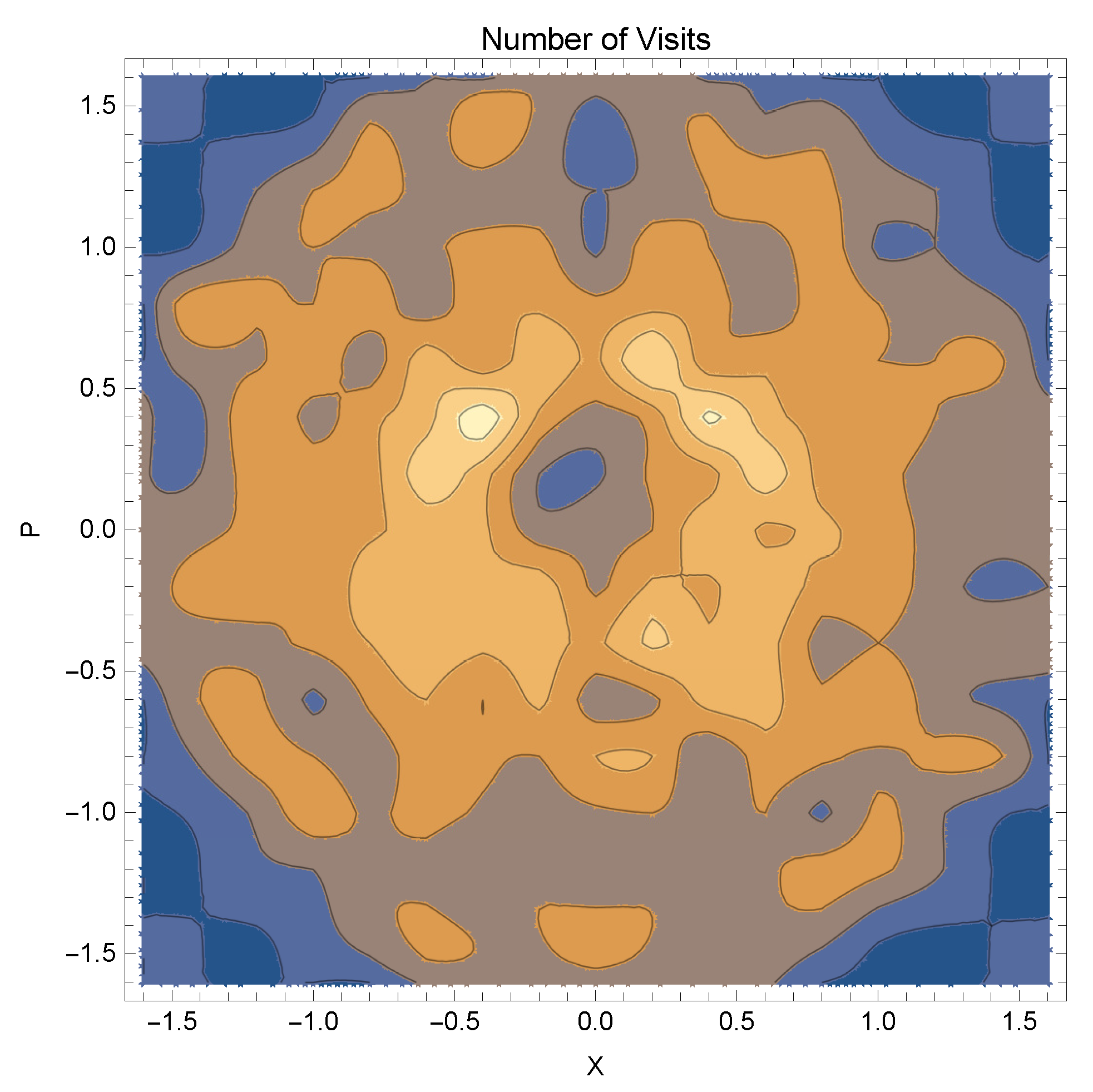
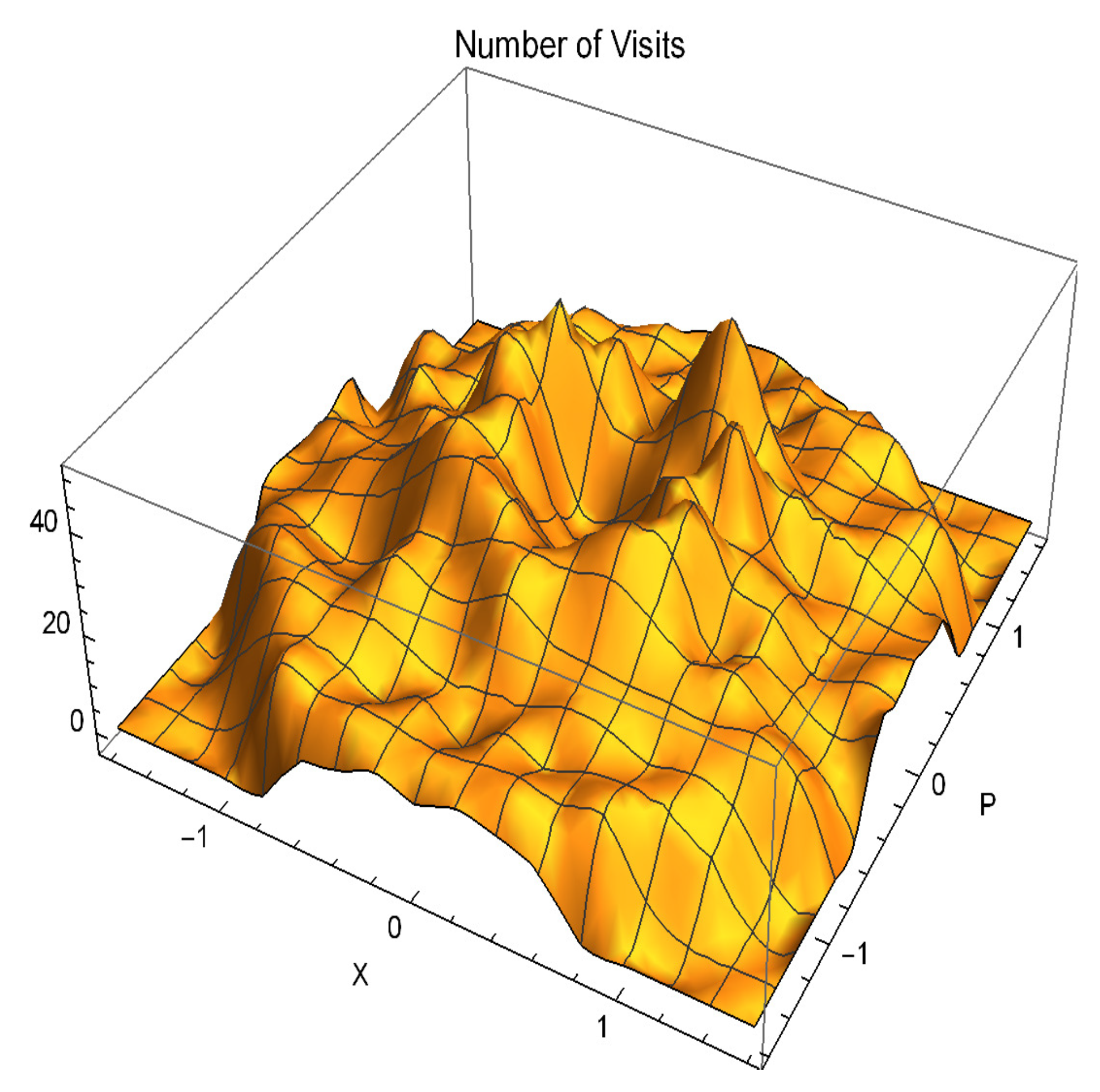
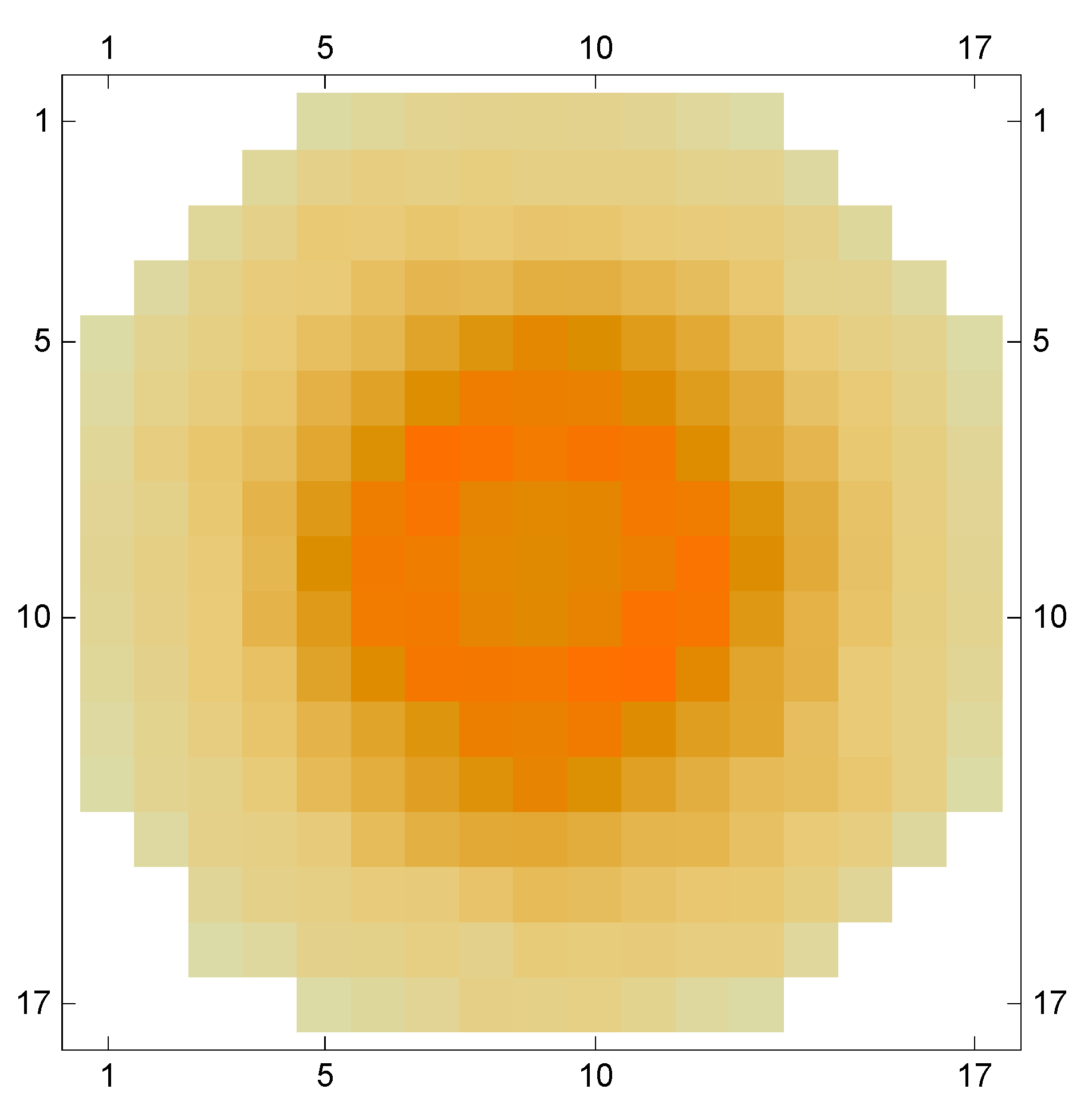
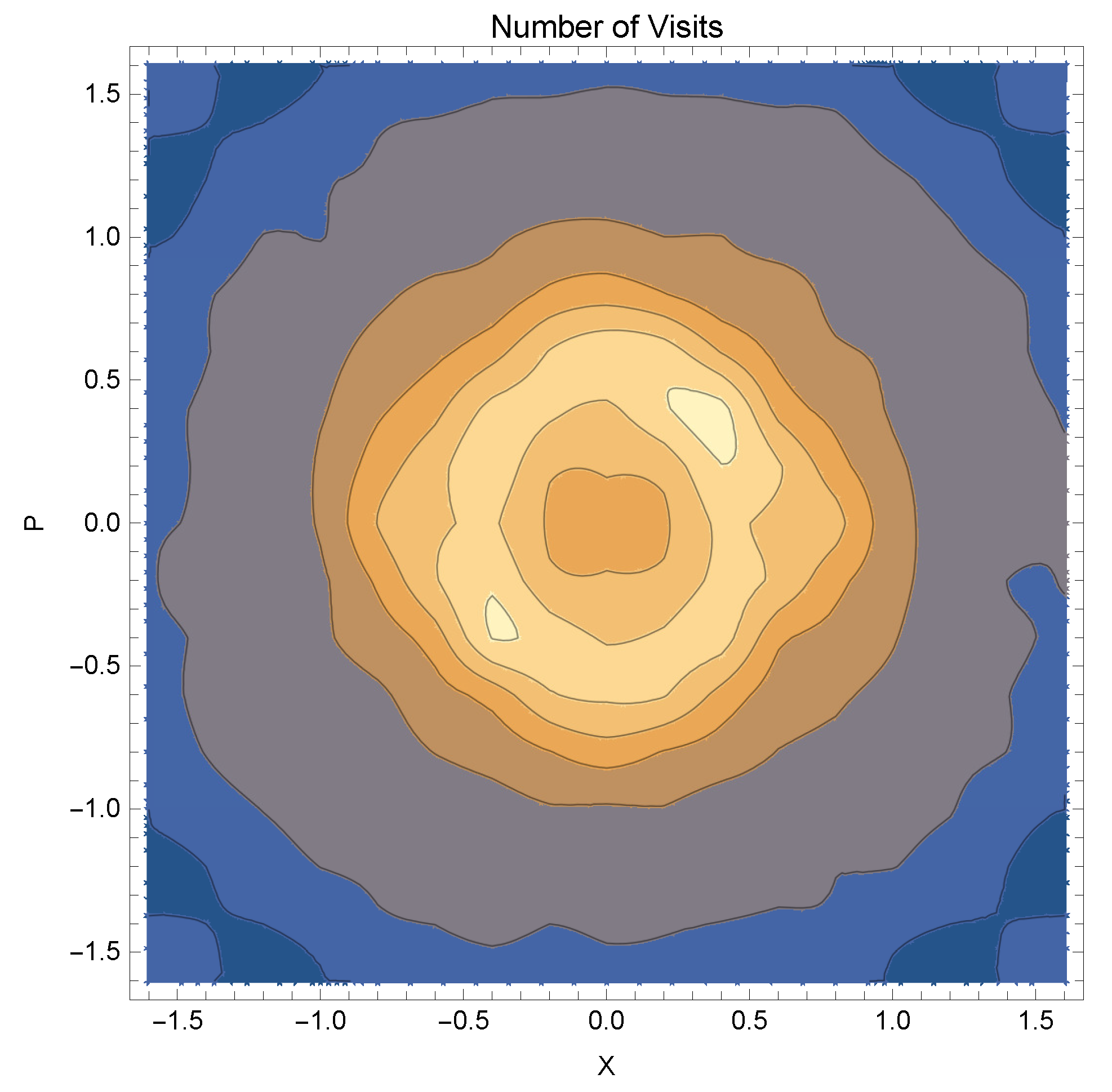
Further three figures shown are, first a matrix plot Figure 2, in which the color depth shows the numerical values of N V over 17 × 17 square positions, a contour plot of the same data in Figure 3 and a 3D plot Figure 4, all three for the parameter values of t r = 4000 , n p = 0.02 , N = 3 . The lesson from each figure, though appearing in different ways, is that (for this choice of parameters ) the trajectory’s visiting numbers are fairly regularly and systematically distributed.(More detailed conclusions are given shortly below.)
In a further task, we have varied the parameters in several modes and obtained further sets of figures. These are presented in Appendix A. One finds that halving either t r or n p from the above values causes to change the distribution of N V qualitatively, in that it is then highly irregular, almost randomly distributed. On the other hand, changing (e.g., increasing from 3 to 5) the size N of the function space seems to have no qualitative effect, although the quasi-periodicity of the sub-system changes thereby and the number of turns [of the order of t r × Ω ] during t r changes. Apparently, this tendency to further density is compensated by the enlargement of the active phase-space.

2.3. N V in the Ensemble Average

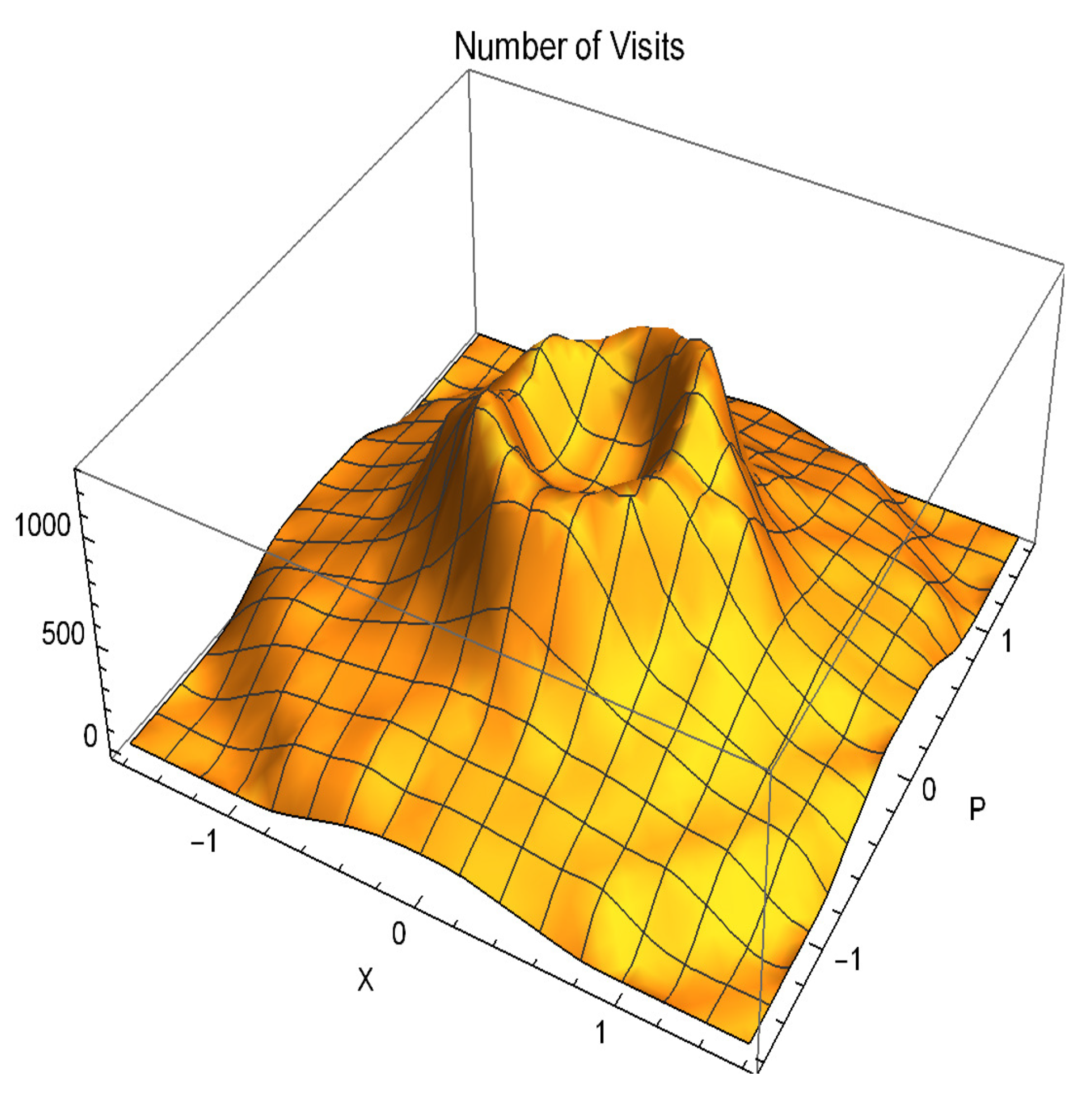
The ensemble average of N V , the partner member in Ergodic Theory, was computed from averaging X 1 r ( t ) in its formula in Equation (6) at some large t and over 100,000 runs in which the phases ϕ n r ( n = 2 , . . , N ; r = 1 , . . . , 100,000) assumed random values, and similarly for the corresponding, derived momenta P 1 r ( t ) . The N V distribution shown on the matrix plot Figure 5, in the contour plot Figure 6 and the 3D plot in Figure 7 is quite regular and tallies reasonably well the time averaged plots shown in the previous three figures.

Partial Summary

The following are the main features of both the time and ensemble averaged results:
(1)
N V vanishes outside a central circular region in the X , P plane, This is, of course, a trivial consequence of the upper bound of the energies in the finite model, alterable only by increase of N.
(2)
N V is (approximately) circularly symmetric and its values are functions of the energies 1 2 ( X 2 + P 2 ) . (Recall that masses and bare frequencies are in the model unity.) With momenta containing also a time dimension, in contrast to the displacements, it seems that this result indicates that the visiting numbers and cumulative sojourn times are commensural, and the system is not subject to what is termed “weakly breaking ergodicity” [21,22,23,24,25,26], in which the two are distinguished.
(3)
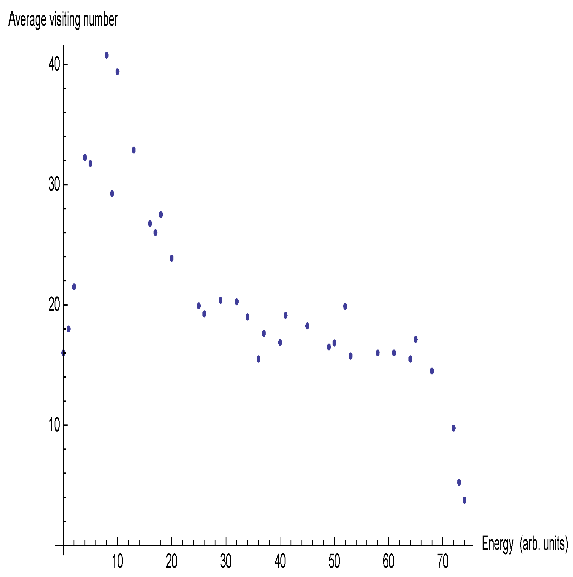
N V is neither monotonic nor uniform along a radial ray (this is not a two dimensionality effect), with a dip at low energies. Whereas the drop at high energies is due to the upper-boundedness of our finite system, the sharp initial rise is remarkable and we wish to claim on the basis of this, that, if in any ensemble averaging the points along a radial ray possess identical measures (as is usually deemed), then for a time integration to be equivalent to that, time durations with low energies must be compensated by an enhancing factor. (The next section argues this from a very different perspective).

2.4. Energy Distribution of NV

This is shown by dots in Figure 8 and it reinforces the claim in item (3), above. The relative smallness of N V even at its peak value of 40 as compared to the number of circling shown in the parametric plot, Figure 1, which is of the order of the run time × frequency and approximately 2000) is remarkable.

3. Quantal: N Spins

For the study of a sub-system inside of a finite reservoir in the quantum setting, a model of interacting spins is considered. The full system is N 1 / 2 -spins (qubits), consisting of one sub-system (labelled 0) interacting with an N 1 sized reservoir of 1 / 2 -spins labelled i ( i = 1 . . . N 1 ) in a form expressed by the following Hamiltonian:
H ( N ) = i = 0 , . . . , N 1 E i σ z i + i , j = 0 , . . . , N 1 ; i j g i j σ x i σ x j
The energy parameters E i in the Hamiltonian are chosen to be of approximately similar magnitudes. The results were tested for several sets of parameters and were found to be qualitatively similar. The Zeeman splitting parameter for the sub-system was set to take the value E 0 = 1 thereby setting the energy scale. The basic energies of the reservoir spins were chosen in a way that avoided any accidental degeneracies in the eigenenergies, namely, E j = 1.5 sin 2 ( 2 π j / 10 ) . For the sub-system-reservoir and inter-reservoir coupling parameters g 0 j and g i j we chose a few combinations of similar magnitudes, with two typical sets given by
g 0 j = 2.5 , g i j = 0.75 ; g 0 j = 3.5 , g i j = 1.5 ; 1 i , j N 1
Numerical diagonalization of the Hamiltonian of Equation (10) yields 2 N ordered energy values W N ( r ) (labelled with the ordinal number index r) for the full system. Their values appear as dots in Figure 9 for N = 5 , 6 , 7 and show a strong initial rise, followed by a more moderate one. Further results were obtained for N = 8 , 9 with similar features; these are not shown in the figure, since their multitude prevents a good visualisation.
A visually determined (not by least square fitting) three-parameter analytical representation of the eigen-energies W N ( r ) of the system as function of its (increasing) serial number r = 0 , . . . , 2 N 1 is
W N ( r ) = W N ( 0 ) + k T ^ log [ 1 + ( A / k T ^ ) r ]
In this only the initial value W N ( 0 ) depends markedly on N, and it is not evident how to assign an intuitive physical meaning to the computed values of this size dependence of the ground state energy. On the other hand, the overall results for most of the computed N’s can be reasonably well fitted with A = 0.15 and k T ^ = 0.45 , with the latter related to the the mean energy. Inverting the above relation, one obtains the cumulative number of eigen-values r r ( W ) as function of the eigen-energies W N :
r ( W N ) = k T ^ A e W N W N ( 0 ) k T ^ 1
The k T ^ symbol for the fitting parameter is suggested by the functional form of the above formula. In the large reservoir limit, for most of the energies the first, exponential term dominates, giving, as expected, an exponential rise of the number of eigen values of the full system, and indeed it was shown by Rechtman and Penrose [42], that for a subsystem in thermal contact with an infinite reservoir at a given temperature, the energy level distribution obeys a Gibbs distribution formula.

3.1. Density of Reservoir-States

With the composite system (sub-system + reservoir) possessing an eigen-energy W N W N ( t o t a l ) , the reservoir’s energy alone is, at any time t, E N W N e ( t ) , having subtracted (with the assumption of simple additivity of the energies) from the composite system’s energy the sub-system’s instantaneous energy e ( t ) . Then substituting in Equation (13), at a time t the r’th eigen-state of the reservoir resides at a height r [ W N e ( t ) ] which is (by neglect of unity in Equation (13)) proportional to
e W N e ( t ) k T ^ r ( t )
In the infinitesimal energy region ( W N , W N + δ E ) the number of reservoir states has then the time dependence of
d r ( W N e ( t ) ) d W N δ E = ( k T ^ ) 1 e W N e ( t ) k T ^ δ E
with a pre-factor that is the energy density (also referred to as the configuration number density) of states in the reservoir. The sub-system density, obtained through weighting (integrating) the reservoir’s configuration number, is called the “reduced density”, or the reduced density matrix (abbreviated RDM) [44]. Due to normalization RDM, time-independent factors can be omitted, requiring a time non-constant weighting in the time-integrated averages.

3.2. A Time-Dependent Configuration Number Argument

Intuitively, the non-uniform time weighting may be claimed to be obvious and by the following reasoning:
For a given total energy W N of the full system, a small sub-system’s instantaneous energy e ( t ) leaves W N e ( t ) energy states for the reservoir (strictly valid under assumption of “weak interaction”). The larger this quantity, the more populous will be the number of reservoir’s state in the neighbour of this energy value, since the number of its configurations increases with energy (and asymptotically does so exponentially). Consequently, the statistical weight of the sub-system regarded at a time when e ( t ) is small is larger than when it is large and the time integration will be under a non-uniform measure, requiring that the time integration be carried out with a non-uniform weighting. In the case of a thermal (infinitely large) reservoir at temperature T, the weighting will be by the well known thermal factor, e [ E ( t o t a l ) e ( t ) ] / k T , as indeed found in Reference [42]. The present work predicates the time-weighting factor for some finite-sized reservoirs.

4. Discussion

While the present work treating finite but large systems is of interest per se, in that it generates numerical data (which is well-nigh impossible for strictly infinite systems), it also sheds light on the ergodic behaviour of infinite systems, such as those in the thermodynamic limit. Regarding the multiple uses in this work of the term “finiteness” there is erstwhile the finiteness of the system size appearing in the title and which had values between 3 and 9 in the worked models. But there is more “finiteness” to note and to describe (yet discounting the finite steps which the Mathematica program employs to generate the trajectory)—there is the run time t r = O ( 1000 ) (measured in units of typical inverse frequencies); then, there is the quantification of “nearness” ( n p = 0.01 0.02 ) measuring the “tolerance” in the numerical “equality” between X 1 ( t ) , P 1 ( t ) along the trajectory and the coordinate values in the classical phase-space X , P (each being typically of the order of unity in the units entering this work), followed by the number [ O ( 20 × 20 ) ] of tiny squares, into which the traversed space-phase domain is partitioned. Ergodicity in its common formulation requires these quantities to be (respectively) infinite or zero. Our results throw light on the role of each of these quantities in achieving, or approaching, ergodicity, when their values are not yet in these limits, but are finite.
Briefly, the onset of ergodicity is critically promoted, expectedly, by the length of the run-time t r and also by softening (increasing) the nearness parameter n p , but apparently not by coupling to additional reservoir degrees of motion (which is done in Appendix A by an enlargement of dimensions of the Hamiltonian matrix from 9 to 25). The reason for the last finding is that while the quasi-periodicity of the almost-periodic functional behaviour of the sub-system is shortened, the active region of phase-space is enlarged.
The evident shortcoming of this study is that it is confined to very particular models (one in the classical, the other in the quantum regime, and at those to rather simple ones), whereas the applicability of ergodic theory seems to be practically unlimited (a rather bizarre case having been mentioned in Reference [16]). This is exemplified by the the variety of systems, both physically realistic and artificial ones, whose ergodic properties were inquired into, a fraction of which only is cited here in the Bibliography through References [22,23,24,25,26]. A further lacuna, noted by a referee, is the absence of boundary effects in the treatment of “symmetry breaking”. A distinguished set of works, assessing the thermalization effects of coupling to a large number of oscillators have led to a Langevin-equation formalism. A more profound statistical analysis of the numerical results awaits future work.
The foregoing considerations regarding “finitenes” have focused mainly on the classical part of this work (Section 2). In the quantal Section 3 the stress is on the claim that the time averaging (performed in one of the two members of the ergodic theorems) is to be weighted in a non-uniform manner: durations at lower energies needing to be additionally weighted, in preference to high energy ones. For the exact formulation we refer to the results in that section, there propped up also by an intuitive argument. Most of the theoricizing on ergodicity is unclear on this point, and is absent in formal expressions in the subject, our personal discussions have revealed skepticism, if not opposition to this claim. The present work should be part in the deliberation of the issue.

Funding

This research received no external funding.

Acknowledgments

Eli Barkai (Bar-Ilan University) is thanked for a careful reading and fruitful comments. Technical, and nonetheless vital, help from Roi Baer, Nadav Katz, Guy Ron (Hebrew University), Asher Yahalom (Ariel University) and Noam Kayzer (Bar-Ilan University) is gratefully noted. The author is indebted to Joel Leibowitz (Rutgers University) for discussion and a challenge to show that time-weighted ergodicity occurs also for classical, non-quantal systems.

Conflicts of Interest

The author declares no conflict of interest.

Appendix A. Proof of Ensemble Construction Rule in Equation (5)

From Equation (6) for X i r ( t ) in the text for a random realization (labelled r) of the i-th local spin, we form the following averages over a large number R of different random realizations:
< r | X 1 r ( 0 ) | 2 > = ( 1 / R ) r = r " n m A i m A i n + sin ϕ n r sin ϕ m r " = ( 1 / R ) n m A i m A i n + r = r " sin ϕ n r " sin ϕ m r = ( 1 / R ) n A i n A i n + r ( sin ϕ n r ) 2 = 1 2
having made use of in the penultimate line the destructive interference of sine cross products and in the last line the unitary property of the transformation matrix A i m , as in Equation (8).
The proof for the second relation Equation (5) goes through in the same way, except for cosine replacing sine and having sandwiched between the transformation matrices the eigen-frequencies Ω n Ω m . The second relation in Equation (8) and our choice of unity in the diagonal elements of the dynamical matrix ensure the verification of Equation (5).

Appendix B. Parameter Dependencies of the Visiting Number NV

A number of computations, analogous to those presented in Section 2, were made in which the parameters of the simulations differed from those in the text, where the tendencies to ergodicities have been established. We recall here those values:
Run-time t r = 4000 (in inverse frequency units); Nearness parameter n p (marking the maximum offset in the configuration values X , P for a “visit” to have taken place) = 0.02 as fraction of typical X , P ’s; the number of coupled oscillators N = 3
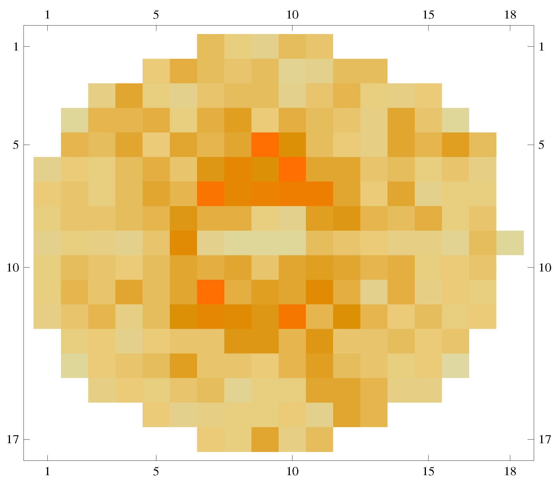
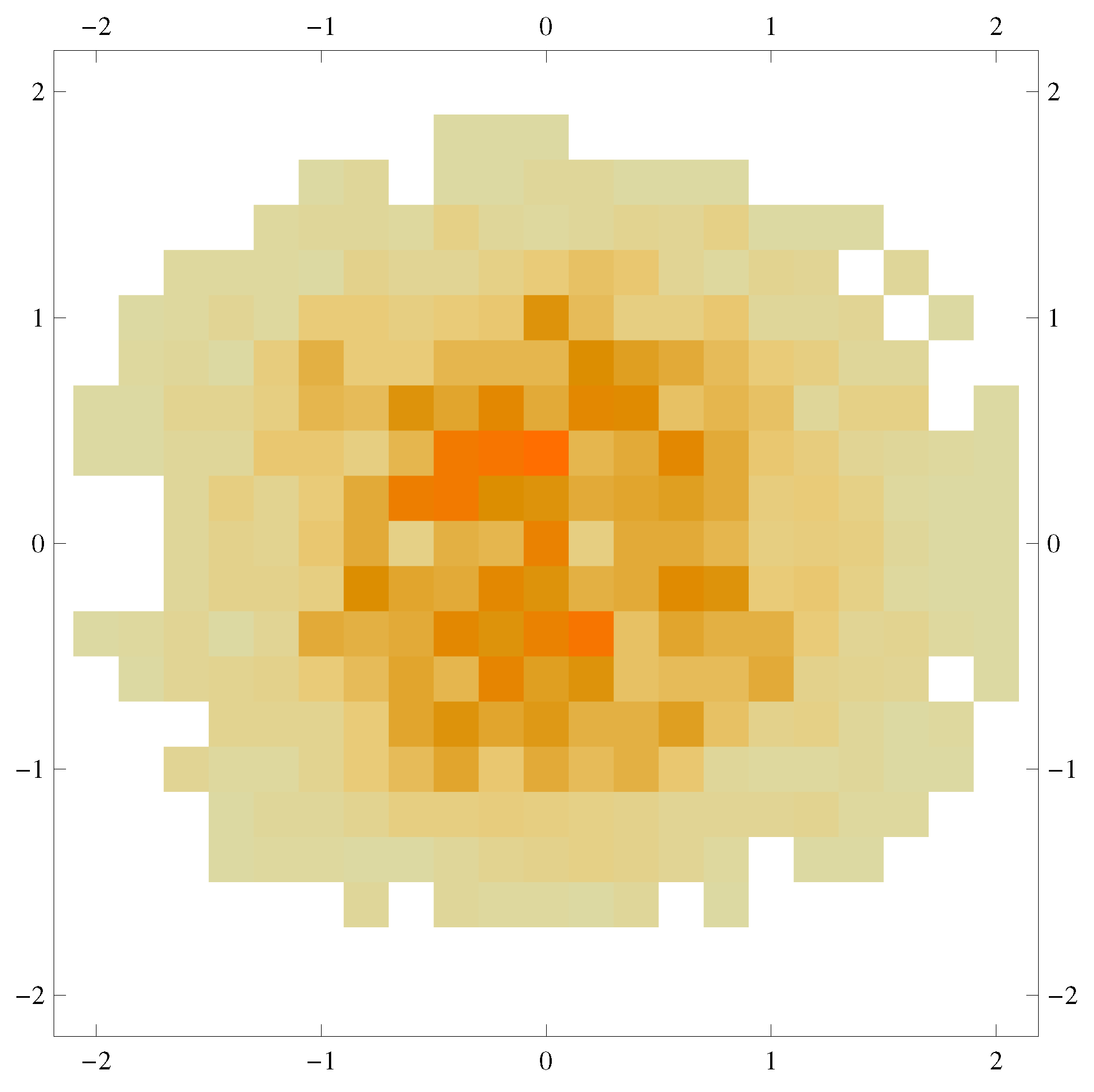
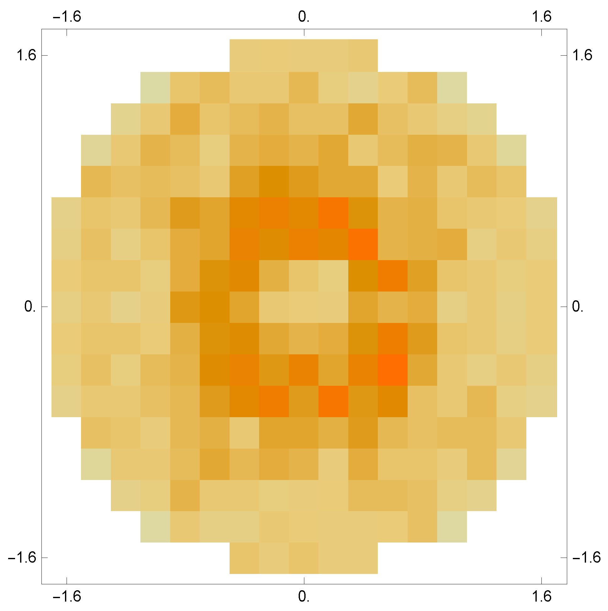
In the following figures one or other parameter is changed, with the following consequences: halving the run time alone to t r = 2000 , as in Figure A1 has a destructive effect on the regularity of visiting times; in effect, the entries in the squares are essentially random values. Likewise, as apparent from Figure A2, stiffening the nearness condition to n p = 0.01 alone will also chaotize the visiting times, eschewing strict ergodicity. An increase in the number of coupled oscillators to N = 5 alone does not appear to promote ergodicity, as evident from Figure A3. Further results and figures were also created and are available upon request. They lead to the net conclusion that an onset of ergodicity is an open possibility also for finite systems, but only upon satisfaction of some quantitative criteria, such as very long run times (in the present instances t r 4000 ) and reasonably broad nearness criteria ( n p 0.02 ).
Figure A1. Visiting numbers under reduced run times. The entries are chaotically distributed.
Symmetry 12 01642 g0a1
Figure A2. Visiting numbers with a stricter nearness criterion for visits. Chaotic entries in the small squares.
Symmetry 12 01642 g0a2
Figure A3. Increasing the number of interacting oscillators alone does not induce order in the basic square entries.
Symmetry 12 01642 g0a3

References

  1. Farquhar, I.E. Ergodic Theory. In Statistical Mechanics: Interscience; Wiley: London, UK, 1964; Chapter 2. [Google Scholar]
  2. Ruelle, D. Ergodic theory of differentiable dynamic systems. Publ. Math. Inst. Hautes éTudes Sci. 1979, 50, 27–58. [Google Scholar] [CrossRef] [Green Version]
  3. Earman, J.; Rédei, M. Why ergodic theory does not explain the success of Statistical Mechanics? Br. J. Phil. Sci. 1996, 47, 63–78. [Google Scholar] [CrossRef] [Green Version]
  4. Malament, D.B.; Zabell, S.L. Why Gibbs averages work -True role of ergodic theory. Philos. Sci. 1980, 47, 339–349. [Google Scholar] [CrossRef]
  5. Moore, C.E. Ergodic theorem, ergodic theory and statistical mechanics. Proc. Natl. Acad. Sci. USA 2015, 112, 1907–1992. [Google Scholar] [CrossRef] [Green Version]
  6. Morasaagh, R.; Schenker, J. Theory of ergodic processes. arXiv 2020, arXiv:2034.14397v2. [Google Scholar]
  7. Szasz, D. Boltzmann’s Ergodic Hypothesis; Preprint ESI: Wien, Austria, 1994; unpublished. [Google Scholar]
  8. Sarig, O.M. Lecture Notes on Ergodic Theory (Lecture Notes 2009). 2009. Available online: https://citeseerx.ist.psu.edu/viewdoc/download?doi=10.1.1.218.752&rep=rep1&type=pdf (accessed on 1 October 2020).
  9. Lee, M.H. Long time behavior, Hermitian modes, Birkhoff’s theorem, many-body response functions and the ergodic condition. Phys. Rev. Lett. 2007, 98, 110403-6. [Google Scholar] [CrossRef]
  10. Lee, M.H. Local dynamics in an infinite harmonic chain. Symmetry 2016, 8, 22. [Google Scholar] [CrossRef] [Green Version]
  11. Von Neumann, J. Proof of the quasi-ergodic hypothesis. Proc. Natl. Acad. Sci. USA 1932, 18, 263–266. [Google Scholar] [CrossRef] [Green Version]
  12. Birkhoff, G.P. Proofs of the ergodic theorem. Proc. Natl. Acad. Sci. USA 1931, 17, 656–660. [Google Scholar] [CrossRef]
  13. Poincaré, H. Sur le probleme des trois corps et les equations de la dynamique. Acta Math. 1890, 13, A3–A270. [Google Scholar]
  14. Boltzmann, L. Uber die mechanishen Analogien der zweiten Haupsatzes der Thermodynamik. J. Math. 1887, 1887, 201–212. [Google Scholar]
  15. Oxtoby, J.; Ulam, S. Measure preserving homeomorphisms and metrical transitivity. Ann. Math. 1974, 42, 874–920. [Google Scholar] [CrossRef]
  16. Paulus, M.P.; Goyer, M.A.; Gold, L.; Mandell, A.J. Application of entropy measures derived from the ergodic theory of dynamical systems to rat locomotive behavior. Proc. Natl. Acad. Sci. USA 1990, 87, 723–727. [Google Scholar] [CrossRef] [PubMed] [Green Version]
  17. Englman, R.; Yahalom, A. Partial decoherence and thermalization through time-domain ergodicity. Phys. Rev. A 2013, 87, 052123. [Google Scholar] [CrossRef] [Green Version]
  18. Englman, R.; Yahalom, A. Open systems’ density matrix properties in a time coarsened formalism. Found. Phys. 2015, 45, 673–690. [Google Scholar] [CrossRef] [Green Version]
  19. Ehrenfest, P.; Ehrenfest, T. Begriffliche Grundlagen der statistishen Auffassung in der Mechanik. Ann. Math. Wiss. 1912, 2, 10–13. [Google Scholar]
  20. Ehrenfest, P.; Ehrenfest, T. The Conceptual Foundations of the Statistical Approach in Mechanics; Moravcsik, M., Translator; Cornell University Press: Ithaca, NY, USA, 1959. [Google Scholar]
  21. Bouchaud, J.P. Weak ergodicity breaking. J. Phys. 1992, 2, 1705–1710. [Google Scholar]
  22. Bel, G.; Barkai, E. Weak ergodicity breaking with deterministic dynamics. Europhys. Lett. 2006, 74, 15–20. [Google Scholar] [CrossRef] [Green Version]
  23. Margolin, G.; Barkai, E. Nonergodicity of a time series obeying Levy statistics. J. Stat. Phys. 2006, 122, 137–167. [Google Scholar] [CrossRef] [Green Version]
  24. Bel, G.; Barkai, E. Weak ergodicity breaking in the continuous time random walk. Phys. Rev. Lett. 2006, 94, 24602. [Google Scholar] [CrossRef] [Green Version]
  25. Rebenstock, A.; Barkai, E. Distribution of time-averaged observables for weak ergodicity breaking. Phys. Rev. Lett. 2009, 99, 210601. [Google Scholar] [CrossRef] [PubMed] [Green Version]
  26. Turner, C.J.; Michailidis, A.A.; Abadin, D.A.; Serbyn, H.M.; Papir, Z. Weakly breaking of ergodicity. Nat. Phys. 2018, 14, 745–748. [Google Scholar] [CrossRef] [Green Version]
  27. Gu, M.; Wiesner, K.; Rieper, E.; Vedral, V. Quantum mechanics can reduce the complexity of classical models. Nat. Commun. 2012, 3, 1–5. [Google Scholar] [CrossRef] [PubMed] [Green Version]
  28. Zhou, H.; Choi, J.; Choi, S.; Landig, R.; Douglas, A.M.; Isoya, J.; Jelezko, F.; Onoda, S.; Sumiya, H.; Cappellaro, P.; et al. Quantum metrology with strongly interacting spin systems. Phys. Rev. X 2020, 10, 031003. [Google Scholar] [CrossRef]
  29. Qiao, H.; Kandel, Y.P.; Deng, K.; Fallahi, S.; Gardner, G.C.; Manfra, M.J.; Barnes, E.; Nichol, J.M. Coherent multispin exchange coupling in a quantum-dot spin chain. Phys. Rev. X 2020, 10, 031006. [Google Scholar]
  30. Deutsch, J.M. Quantum statistical mechanics in a closed system. Phys. Rev. A 1991, 43, 2046–2049. [Google Scholar] [CrossRef]
  31. Srednicki, M. Chaos and quantum thermalization. Phys. Rev. E 1994, 50, 888–901. [Google Scholar] [CrossRef] [Green Version]
  32. Tasaki, H. From quantum mechanics to the canonical distribution: General picture and a rigorous example. Phys. Rev. Lett. 1998, 80, 1373–1376. [Google Scholar] [CrossRef] [Green Version]
  33. Rigol, M.; Dunjko, V.; Olshani, M. Thermalization and its mechanism for generic isolated quantum systems. Nature 2008, 452, 854–858. [Google Scholar] [CrossRef] [Green Version]
  34. Popescu, S.; Short, A.J.; Winter, A. Entanglement and the foundations of statistical mechanics. Nat. Phys. 2006, 2, 754–758. [Google Scholar] [CrossRef] [Green Version]
  35. Linden, N.; Popescu, S.; Short, A.J.; Winter, A. Quantum mechanical evolution towards thermal equilibrium. Phys. Rev. A 2009, 79, 061103. [Google Scholar] [CrossRef] [PubMed] [Green Version]
  36. Sirker, J.; Konstantinidis, N.P.; Andrashko, F.; Sedlmayer, N. Localization and thermalization in closed quantum mechanical systems. arXiv 2013, arXiv:1303.3064v3. [Google Scholar]
  37. Alba, V. Eigenstate thermalization hypothesis (ETH) and integrability in quantum spin chains. arXiv 2013, arXiv:1409.6096 v1. [Google Scholar]
  38. Beugeling, W.; Moessner, R.; Haque, M. Finite size scaling of eigensate thermalization. Phys. Rev. E 2014, 89, 042112. [Google Scholar] [CrossRef] [PubMed] [Green Version]
  39. Breuer, H.P.; Petruccione, F. The Theory of Open Quantum Systems; Oxford University Press: Oxford, UK, 2007. [Google Scholar]
  40. Lanting, T.; Przybysz, A.J.; Smirnov, A.Y.; Spedalieri, F.M. Entanglement in a quantum annealing processor. Phys. Rev. X 2014, 4, 02104. [Google Scholar] [CrossRef] [Green Version]
  41. Bertana, S.; Gambarelli, S.; Mitra, T.; Tsukerblat, B.; Müller, A.; Barbara, B. Quantum oscillations in a molecular magnet. Nature 2008, 453, 203–206. [Google Scholar] [CrossRef] [Green Version]
  42. Rechtman, P.; Penrose, O. Continuity of the temperature and derivation of the Gibbs canonical distribution in classical statistical mechanics. J. Stat. Phys. 1978, 19, 359–366. [Google Scholar] [CrossRef]
  43. Leggett, A.J.; Chakravarty, S.; Dorsay, A.P.; Fisher, M.P.A.; Garg, A.; Zwerger, W. Dynamics of the dissipative two-level system. Rev. Mod. Phys. 1987, 59, 1. [Google Scholar] [CrossRef]
  44. Irish, E.K.; Gea-Banacloche, J.; Martin, I.; Schwab, K.C. Dynamics of a two-level system strongly coupled to a high-frequency quantum oscillator. Phys. Rev. B 2005, 72, 195410. [Google Scholar] [CrossRef] [Green Version]
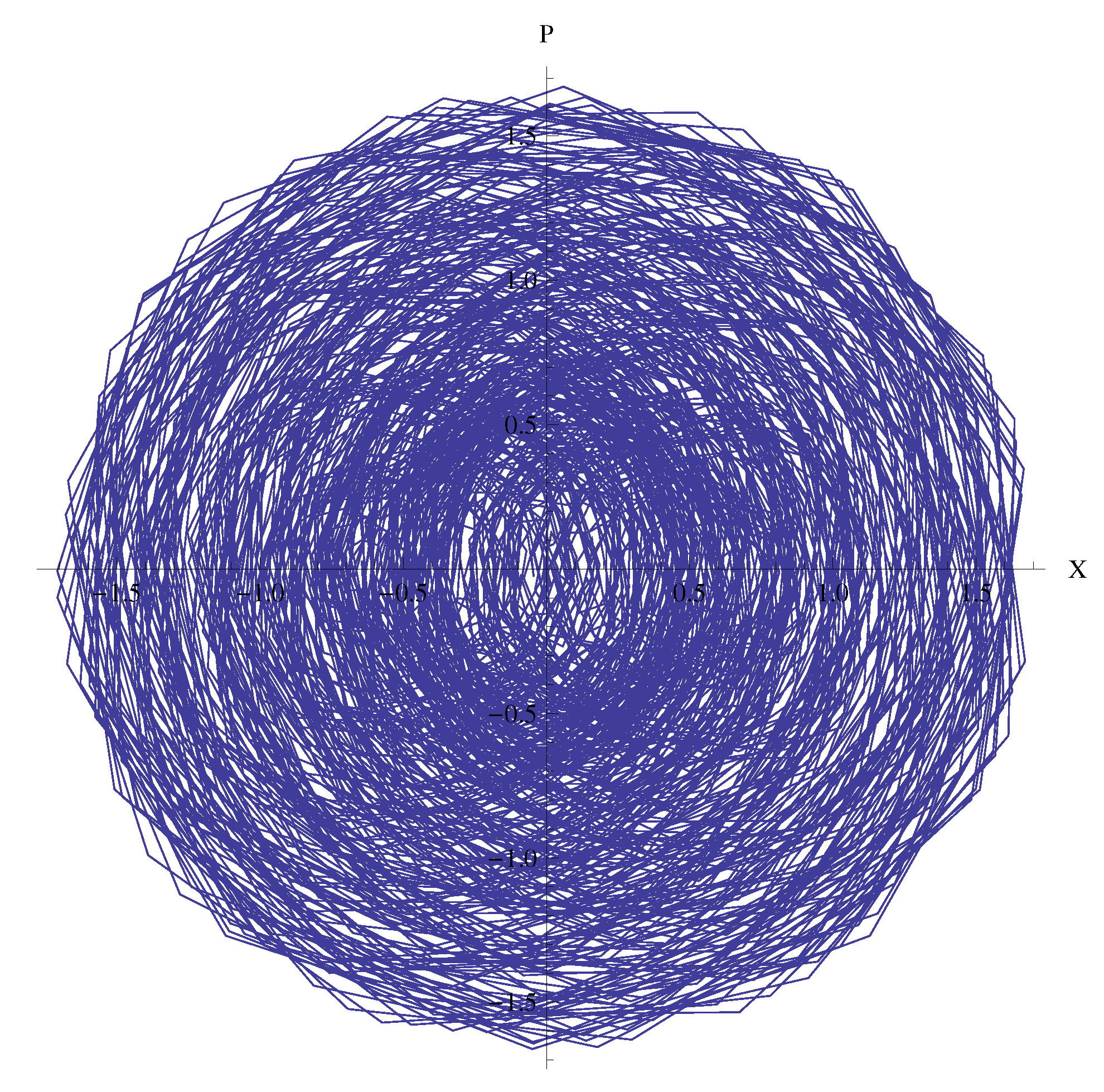
Figure 1. The trajectory trace of the sub-system in phase- space plane at a run time t r = 2000 in units of inverse frequencies and number of oscillators N = 3 . Overall, a dense covering is apparent.
Symmetry 12 01642 g001
Figure 2. Visiting number N V distributed over the phase-space, plotted by a matrix plot in which the color depths represent the numerical values in the small squares (deeper color meaning higher values). Plotted for a nearness parameter n p = 0.02 and run time t r = 4000 (in reciprocal units of the frequencies). N V is seen to be distributed regularly. Detailed discussion is in the text.
Symmetry 12 01642 g002
Figure 3. A contour plot for the visiting number N V distribution in the phase space plane, using the same parameters and data as in the previous figure.
Symmetry 12 01642 g003
Figure 4. A three dimensional plot for the visiting number N V distribution in the phase space plane, using the same parameters and data as in the previous figure.
Symmetry 12 01642 g004
Figure 5. MatrixPlot for the visiting numbers of a large ensemble (for a solutions of the same Hamiltonian, but 100,000 different initial conditions for the dynamic variables [ X 1 ( t ) , P 1 ( t ) ]), with nearness parameter n p = 0.02 . A fairly regular radial dependence is shown, with nearly circular shape (discussed in the text). The number of visits at a typical phase - space point is 400 with a peak of 1152 (in the course of 10 5 runs!).
Symmetry 12 01642 g005
Figure 6. Distribution of visiting numbers N V at a given time averaged over 10 5 randomly chosen members in the ensemble. n p = 0.02 .
Symmetry 12 01642 g006
Figure 7. A 3D plot of the previous.
Symmetry 12 01642 g007
Figure 8. Distribution of visiting numbers N V as function of the energy 1 2 ( X 1 ( t ) 2 + P 1 ( t ) 2 ) .
Symmetry 12 01642 g008
Figure 9. Dots: Eigenenergies (in arbitrary units, numbering 2 N values) plotted against the serial number r for an N- spin system ( N = 5 , 6 , 7 ). There are two regions: the first sharply linearly increasing, followed by a more moderate tendency to rise. Curve to fit the dot values (after their arbitrary shifts vertically) described in the text.
Symmetry 12 01642 g009