New Online Streaming Feature Selection Based on Neighborhood Rough Set for Medical Data

Abstract

Not all features in many real-world applications, such as medical diagnosis and fraud detection, are available from the start. They are formed and individually flow over time. Online streaming feature selection (OSFS) has recently attracted much attention due to its ability to select the best feature subset with growing features. Rough set theory is widely used as an effective tool for feature selection, specifically the neighborhood rough set. However, the two main neighborhood relations, namely k-neighborhood and $\delta$ neighborhood, cannot efficiently deal with the uneven distribution of data. The traditional method of dependency calculation does not take into account the structure of neighborhood covering. In this study, a novel neighborhood relation combined with k-neighborhood and $\delta$ neighborhood relations is initially defined. Then, we propose a weighted dependency degree computation method considering the structure of the neighborhood relation. In addition, we propose a new OSFS approach named OSFS-KW considering the challenge of learning class imbalanced data. OSFS-KW has no adjustable parameters and pretraining requirements. The experimental results on 19 datasets demonstrate that OSFS-KW not only outperforms traditional methods but, also, exceeds the state-of-the-art OSFS approaches.

1. Introduction

The number of features increases with the growth of data. A large feature space can provide much information that is useful for decision-making [1,2,3], but such a feature space includes many irrelevant or redundant features that are useless for a given concept. It is of necessity to remove the irrelevant features so that the curse of dimensionality can be relieved. This motivates some sort of research for feature selection methods. Feature selection, as a significant preprocessing step of data mining, can select a small subset, including the most significant and discriminative condition features [4]. Traditional methods are developed based on the assumption that all features are available. Many typical approaches exist, such as ReliefF [5], Fisher Score [6], mutual information (MI) [4], Laplacian Score [7], LASSO [8], and so on [9]. The main benefits of feature selection include speeding up the model training, avoiding overfitting, and reducing the impact of dimensionality during the process of data analysis [4].

However, features in many real-world applications are individually generated one-by-one over time. Traditional feature selection can no longer meet the required efficiency with the growing volume of features. For example, in the medical field, a doctor cannot easily obtain the entire features of a patient. In bioinformatic and clinical medicine situations, acquiring the entire features in a feature space is expensive and inefficient because of high-cost laboratory experiments [10]. In addition, for the task of medical image segmentation, acquiring the entire features is infeasible due to the infinite number of filters [11]. Furthermore, the symptom of a patient persistently changes over time during the treatment, and judging whether the feature contains useful information is essential for identifying the patient’s disease after a new feature has emerged [12]. In these cases, waiting a long time until entire features are available and then performing the feature selection process is the primary method.

Online streaming feature selection (OSFS), presenting a feasible precept to solve feature streaming in an online way, has recently attracted wide concern [13]. The OSFS method must meet the following three criteria [14]: (1) Not all features are available, (2) the efficient incremental updating process for selected features is essential, and (3) accuracy is vital each time.

Many previous studies have proposed some different OSFS methods. For example, a grafting algorithm [15], which employed a stagewise gradient descent approach to feature selection, during which a conjugate gradient procedure was used to carry out its parameters. However, as well as the grafting algorithm, both fast OSFS [16] and a scalable and accurate online approach (SAOLA) [13] need to specify some parameters, which requires the domain information in advance. Rough set (RS) theory [17], which is an effective mathematic tool for features selection, rules extracting, or knowledge acquisition [18], needs no domain knowledge other than the given datasets [19]. In the real world, we usually encounter many numerical features in datasets, such as medical datasets. Under this circumstance, a neighborhood rough set is feasible to analyze discrete and continuous data [20,21]. Nevertheless, all these methods proposed have some adjustable parameters. Considering that selecting unified and optimal values for all different datasets is unrealistic [22], a new OSFS method based on an adapted neighborhood rough set is proposed, in which the number of neighbors for each object is determined by its surrounding instance distribution [22]. Furthermore, in the view of multi-granulation, multi-granulation rough sets is used to compute the neighborhoods of each sample and extract neighborhood size [23]. For the above OSFS methods based on neighborhood relation, dependency degree calculation is a key step. However, very little work has considered the neighborhood structure in the granulation view during this calculation. In additional, the phenomenon of uneven distribution of some data, including medical data, is common, and few works focus on the challenge of the uneven distribution of data.

In this paper, focusing on the strength and weakness of the neighborhood rough set, we proposed a novel neighborhood relation. Further, a weighted dependency degree was developed by considering the neighborhood structure of each object. Finally, our approach, named OSFS-KW, was established. Our contributions were as follows:

(1)

We proposed a novel neighborhood relation, and on this basis, we developed a weighted dependency computation method.

(2)

We developed an OSFS framework, named OSFS-KW, which can select a small subset made up of the most significant and discriminative features.

(3)

The OSFS-KW was established based on [24] and can deal with the class imbalance problem.

(4)

The results indicate that the OSFS-KW cannot only obtain better performance than traditional feature selection methods but, also, better than the state-of-the-art OSFS methods.

The remainder of the paper is organized as follows. In Section 2, we briefly review the main concepts of neighborhood RS theory. Section 3 discusses our new neighborhood relations and proposes the OSFS-KW. Then, Section 4 performs some experiments and discusses the experimental results. Finally, Section 5 concludes the paper.

2. Background

Neighborhood RS has been proposed to deal with numerical data or heterogeneous data. In general, a decision table (DT) for classification problem can be represented as $IS=<U,R,V,f>$ [25], where $U$ is a nonempty finite set of samples. R can be divided condition attributes C and decision attributes D, $C\cap D=\varnothing$. $V=\cup \{V_r|r\in R\}$ is a set of attributes domains, such that $V_r$ denotes the domains of an attribute r. For each $r\in R$ and $x\in U$, a mapping $f:U\times R\to V$ denotes an information function.

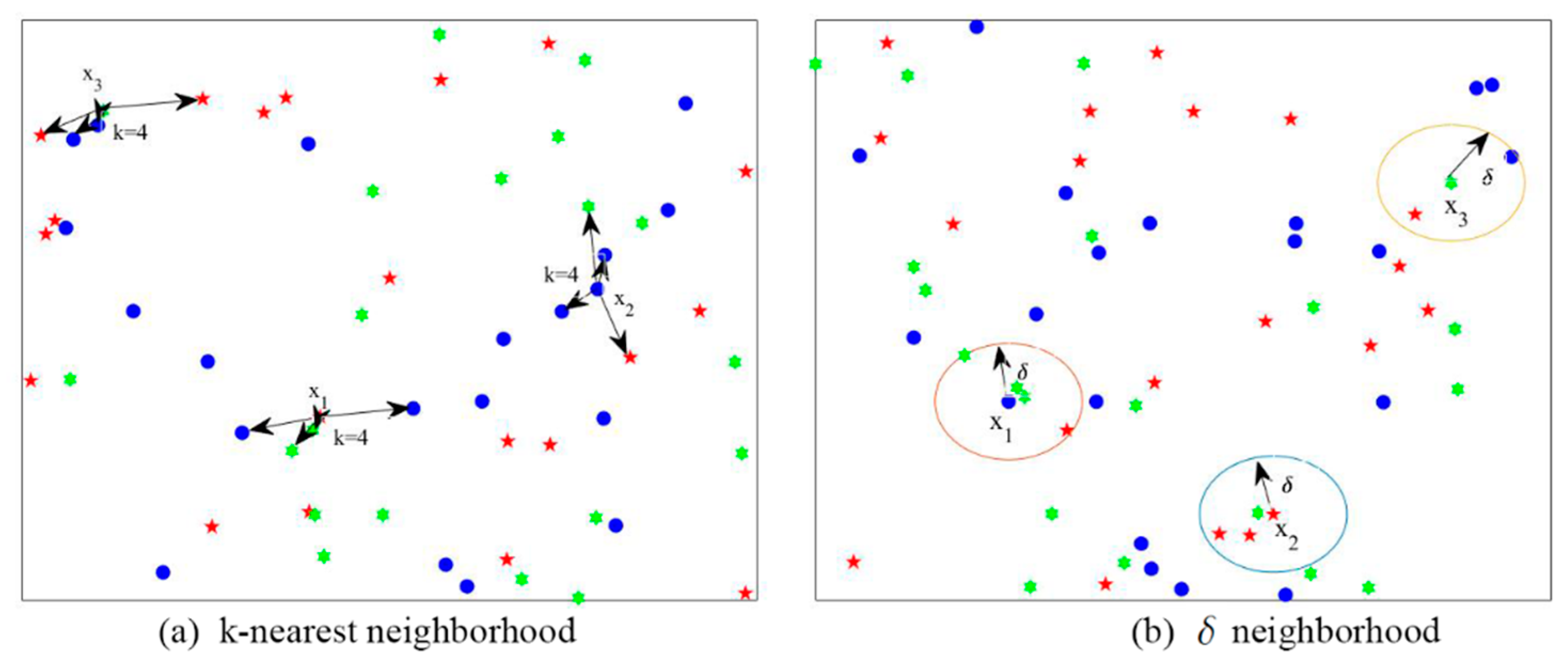
There are two main kinds of neighborhood relations: (1) the k-nearest neighborhood relation shown in Figure 1a and (2) the $\delta$ neighborhood relation shown in Figure 1b.

Figure 1. Two kinds of neighborhood relations.

Definition 1 

[26]. Given DT, a metric $△$ is a distance function, and △(x, y) represents the distance between x and y. Then, for $\forall x,y,z\in U$, it must satisfy the following:

(1) 

$△(x,y)\ge 0$, when$x=y$and$△(x,y)=0$,

(2) 

$△(x,y)=△(\mathrm{y},x)$, and

(3) 

$△(x,z)\le △(x,y)+△(y,z)$.

Definition 2 

($\delta$ neighborhood [22]). Given DT, a feature subset $B\subseteq C$, the neighborhood ${\delta }_B^r(x)$ of any object $x\subseteq U$ is defined as follows:

$${\delta }_B^r(x)=\{y|{△}_B(x,y)\le r,y\in U,y\ne x\}$$

(1)

where $r$ is the distance radius, and ${\delta }_B^r(x)$ satisfies:

(1) 

$y\in {\delta }_B^r(x)\Rightarrow x\in {\delta }_B^r(y)$,

(2) 

$1\le card({\delta }_B^r(x))\le card(U)$, where$card(•)$denotes the number of elements in the set, and

(3) 

$\underset{x\in U}{\cup }{\delta }_B^r(x)=U$.

Definition 3 

(k-nearest neighborhood [22]). Given DT and $B\subseteq C$, the k-nearest neighborhood ${\mathbb{K}}_B^k(x)$ of any object $x\subseteq U$ on the feature subset $B$ is defined as follows:

$${\mathbb{K}}_B^k(x)=\{y|y\in MI{N}_k\{{\Delta }_B(x,y)\},y\in U,y\ne x\}$$

(2)

where $MI{N}_k\{{\Delta }_B(x,y)\}$ represents the k neighbors closest to $x$ on a subset B, and ${\mathbb{K}}_B^k(x)$ satisfies:

(1) 

${\mathbb{K}}_B^k(x)\ne \varnothing$,

(2) 

$card({\mathbb{K}}_B^k(x))=k$, and

(3) 

$\underset{x\in U}{\cup }{\mathbb{K}}_B^k(x)=U$.

Then, the concepts of the lower and upper approximations of these two neighborhood relations are defined as follows:

Definition 4. 

Given DT, for any $X\subseteq U$, two subsets of objects, called the lower and upper approximations of$X$with regard to the$\delta$neighborhood relation, are defined as follows [27]:

$$\underset{\_}{B_{\delta }}X=\{x_i|\delta (x_i)\subseteq X,x_i\in U\}$$

(3)

$$\overline{B_{\delta }}X=\{x_i|\delta (x_i)\cap X\ne \varnothing ,x_i\in U\}$$

(4)

If$x\in \underset{\_}{B_{\delta }}X$, then$x$certainly belongs to$X$, but if$x\in \overline{B_{\delta }}X$, then it may or may not belong to$X$.

Definition 5. 

Given DT, for any $X\subseteq U$, the lower and upper approximations concerning the k-nearest neighborhood relation are defined as [24]:

$$\underset{\_}{B_{\mathbb{k}}}X=\{x_i|\mathbb{k}(x_i)\subseteq X,x_i\in U\}$$

(5)

$$\overline{B_{\mathbb{k}}}X=\{x_i|\mathbb{k}(x_i)\cap X\ne \varnothing ,x_i\in U\}$$

(6)

Figure 1a shows that the k-nearest neighbor (k = 4) samples of $x_1$,$x_2$, and $x_3$ have different class labels. In detail, the k-nearest neighborhood samples of $x_1$are from class$C_2$with the mark “·” and class$C_3$with the mark “🟌”; k-nearest neighborhood samples of$x_2$are from classes,$C_2$,$C_3$, and$C_1$with the mark “★”; the k-nearest neighbor samples of$x_3$are from classes$C_1$and$C_2$. Figure 1b depicts that all$\delta$neighbor samples of$x_1$,$x_2$,and$x_3$also come from different class labels. We define the samples of$x_1$,$x_2$, and$x_3$as all the boundary objects. The size of the boundary area can increase the uncertain in DT, because it reflects the roughness of$X$in the approximate space.

By Definition 5, The object space X can be partitioned into positive, boundary, and negative regions [28], which are defined as follows, respectively:

$$PO{S}_B(X)=\underset{\_}{B}X$$

(7)

$$BO{U}_B(X)=\overline{B}X-\underset{\_}{B}X$$

(8)

$$NE{G}_B(X)=U-\overline{B}X$$

(9)

In the data analysis, computing dependencies between attributes is an important issue. We give the definition of the dependency degree as follows:

Definition 6. 

Given DT, for any $B\subseteq C$, the dependency degree of$B$to decision attribute set$D$is defined as [22]

$${\gamma }_B(D)=\frac{CARD(PO{S}_B(D))}{CARD(U)}$$

(10)

The aim of the feature selection is to select a subset$B$from$C$and gain the maximal dependency degree of$B$to$D$. Since the features are available one-by-one over time, it is a necessity to measure each feature’s importance in the candidate features.

Definition 7. 

Given DT, for$B\subseteq C$and$D$, the significance of a feature$c$$(c\in B)$to$B$is defined as follows [22]:

$${\sigma }_B(D,c)={\gamma }_B(D)-{\gamma }_{B\backslash \{c\}}(D)$$

(11)

In a real application, specifically in the medical field, the instances are often unevenly distributed in the feature space; that is, the distribution around some example points is sparse, while the distribution around others is tight. 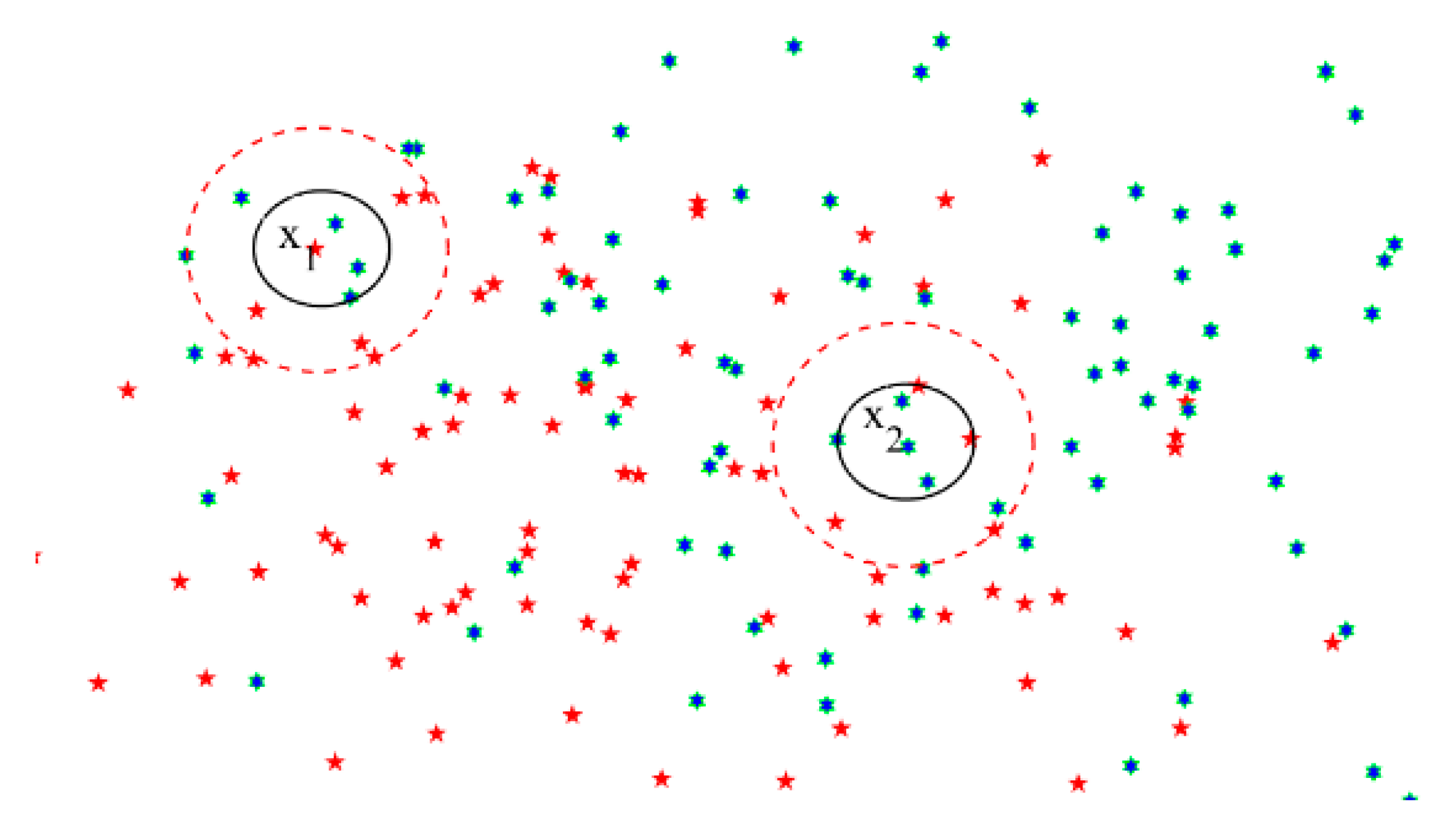Neither the k-nearest neighborhood relation nor the $\delta$ neighborhood relation can portray sample category information well, since the setting of the parameters like r and k can hardly meet both the sparse and tight distributions. For example, the feature space has two classes, as shown in Figure 2—namely, red and green. Red and green represent two different classes respectively, which have different symbols including pentacle and hexagon as well. Around a sample point $x_1$, the sample distribution is sparse. The three nearest points to $x_1$ all have different class from $x_1$. If applying the k-nearest neighborhood relation (k = 3), $x_1$ will be misclassified. However, if we employ the δ neighborhood relation method, then the category of $x_1$ is consistent with that of most samples in the neighbors of $x_1$. On the other hand, the sample distribution around point $x_2$ is tight, and two class samples are included in its neighborhood, and sample $x_2$ will be misclassified when applying the $\delta$ neighborhood relation denoted by the red circle. In fact, if applying the k-nearest neighborhood relation (k = 3), $x_2$ will be classified correctly. Therefore, in Section 3, we proposed a novel neighborhood rough set combining the advantages of the k-nearest neighborhood rough set and the $\delta$ neighborhood rough set.

Figure 2. Distribution of the two class examples.

3. Method

In this section, we initially introduce a definition of OSFS. Then, we propose a new neighborhood relation and an approach of a weighted dependency degree. Based on three evaluation criteria—namely, maximal dependency, maximal relevance, and maximal significance—our new method OSFS-KW is presented finally.

3.1. Problem Statement

$D{S}_t=(U_t,A_t,V_t)$ denotes the decision system (DS) at time t, where $A_t=C_t\cup D_t$ is a feature space including the condition feature $C_t$ and decision feature $D_t$. $U_t=\{x_1,x_2,\dots ,x_{n_t}\}$ is a nonempty finite set of objects. A new feature arrives individually, while the number of objects in $U_t$ is fixed. OSFS aims to derive a mapping of $f_t^{\prime }:x_i\to D (x_i\in U)$ at each timestamp t, which obtains an optimal subset of features available so far.

Contrary to the traditional feature selection methods, we cannot access the full feature space in the scenarios of the OSFS. However, the two main neighborhood relations cannot make up the shortage caused by the uneven distribution data. Moreover, the class imbalanced issue of medical data is common. For example, abnormal cases attract more attention than the normal ones in the field of medical diagnosis. It is also crucial for the proposed framework to handle the class imbalanced problem.

3.2. Our New Neighborhood Relation

3.2.1. $k-\delta$ Neighborhood Relation

The standard European distance method is applied to eliminate the effect of variance on the distance among the samples. Given any samples $x_i$ and $x_j$, and an attribute subset $c\in C$, the distance between $x_i$ and $x_j$ is defined as follows:

$${\Delta }_B(x_i,x_j)=\sqrt{{\displaystyle {\sum }_{c\in B}{(\frac{f(x_i,c)-f(x_j,c)}{{\sigma }_c})}^2}}$$

(12)

where $f(x_i,c)$ denotes the values of x_i relative to the attribute c, and ${\sigma }_c$ represents standard deviation of attribute c.

To overcome the challenge of the uneven distribution of medical data, we proposed a novel neighborhood rough set as follows.

Definition 8. 

Given a decision system$DS=\{U,C,D,f\}$, where$U=\{x_1,x_2,x_3,\dots ,x_n\}$is the finite sample set,$B\in C$is a condition attribute subset, and$D$is the decision attribute set, the$k-\delta$neighborhood relation is defined as follows:

$${\kappa }_B(x_i)=\{x_j\in U|x_j\in {\delta }_B^r(x_i)\cap {\mathbb{k}}_B^k(x_i)\}$$

(13)

where${\delta }_B^r(x_i)$is defined as Definition 2, and${\mathbb{k}}_B^k(x)$is defined as Definition 3.$k=0.15\ast n$, where$n$is the number of instances.

Meanwhile, based on [22],$r=1.5\ast G_{mean}$and G_mean are defined as follows:

$$G_{mean}=\frac{G_{\max }-G_{\min }}{n-1}$$

(14)

More specifically,$G_{\max }$represents the maximum distance from$x_i$to its neighbors, and$G_{\min }$denotes the minimum distance from$x_i$ to its neighbors.

Definition 9. 

Given$DS=\{U,C,D,f\}$and its neighborhood relations$R$on$U$, for$X\subseteq U$, the lower and supper approximation regions of$X$in terms of the$k-\delta$neighborhood relation are defined as follows:

$$\underset{\_}{B_{\kappa }X}=\{x_i|{\kappa }_B(x_i)\subseteq X,x_i\in U\}$$

(15)

$$\overline{B_{\kappa }X}=\{x_i|{\kappa }_B(x_i)\cap X\ne \varnothing ,x_i\in U\}$$

(16)

Similar to Definition 4,$\underset{\_}{B_{\kappa }X}$is also called the positive region, denoted by$PO{S}_B^{\kappa }\left(D\right)$.

3.2.2. Weighted Dependency Computation

The traditional dependency degree only considers the samples correctly classified instead of that of neighborhood covering. To solve this problem, we propose an approach of weighted dependency degree, which considers the granular information for features.

Definition 10. 

Given$DS=\{U,C,D,f\}$, the weighted dependency of$B\in C$is defined as follows:

$${\tau }_B^{\kappa }(D)=w(B)·{\gamma }_B^{\kappa }(D)$$

(17)

where

$$w(B)={\log }_2(2-\phi (B))$$

(18)

$${\gamma }_B^{\kappa }(D)=\frac{CARD(PO{S}_B^{\kappa }\left(D\right))}{CARD(U)}$$

(19)

$$\phi (B)={\displaystyle {\sum }_{\mathrm{i}=1}^{\left|U\right|}\frac{CARD({\kappa }_B(x_i))}{CARD{(U)}^2}}$$

(20)

Theorem 1. 

Given$DS=\{U,C,D,f\}$,$P\subseteq O\subseteq U$. The weight$w(·)$is monotonic, defined as follows:

$$w(P)\le w(O)$$

(21)

Proof. 

According to the monotonicity of neighborhood relation defined in Definition 8, ${\kappa }_O(x_i)\subseteq {\kappa }_P(x_i)$ and $\therefore CARD({\kappa }_O(x_i))\le CARD({\kappa }_P(x_i))$. According to Equation (20), $\phi (O)\le \phi (P)$. Considering Definition 10, $0<\phi (O)\le 1$, $0<\phi (P)\le 1$, and $\therefore 0\le w(P)={\log }_2(2-\phi (P))\le w(O)={\log }_2(2-\phi (O))<1$.  □

Theorem 2. 

Given$DS=\{U,C,D,f\}$,$B\subseteq C$. Then,${\tau }_B^{\kappa }(D)={\tau }_C^{\kappa }(D)$is equivalent to${\gamma }_B^{\kappa }(D)={\gamma }_C^{\kappa }(D)$, and${\log }_2(2-\phi (P))={\log }_2(2-\phi (O))$.

The proof of Theorem 2 is easy according to the monotonicity of the neighborhood relation and Theorem 1.

Definition 11. 

Given$B\subseteq C$and a decision attribute set$D$, the significance of feature c$(c\in B)$to$B$can be rewritten as follows:

$${\sigma }_B(D,c)={\tau }_B^{\kappa }(D)-{\tau }_{B\backslash \{c\}}^{\kappa }(D)$$

(22)

3.3. Three Evaluation Criteria

During the OSFS process, many irrelevant and redundant features should be removed for high-dimensional datasets. There are three evaluation criteria used during the process, such as max-dependency, max-relevance, and max-significance.

3.3.1. Max-Dependency

$C=\{c_1,c_2,\dots ,c_m\}$ denotes the set of m condition attributes. The task of OSFS is to find a feature subset $B\subseteq C$, which has the maximal dependency $\mathbb{D}$ on the decision attributes set $D$. At the moment, the number of features denoted as d in the feature space should be as small as possible.

$$\max \mathbb{D}(B,D),\mathbb{D}={\tau }_B(D)$$

(23)

where ${\tau }_B(D)$ denotes the weighted dependency between the attribute subset B and target class label $D$. The dependency $\mathbb{D}$ can be rewritten as ${\tau }_{B_t}(D)$, where $B_t=\{B_{t-1},c_t\}$. Hence, the increment search algorithm optimizes the following problem for selecting the $t\mathrm{th}$ feature from the attribute set $\{C-B_{t-1}\}$:

$$\underset{c_i\in \{C-B_{t-1}\}}{\max }\{{\tau }_{\{B_{t-1},c_i\}}(D)\}$$

(24)

which is also equivalent to optimizing the following problem:

$$\underset{c_i\in \{C-B_{t-1}\}}{\max }\{{\tau }_{\{B_{t-1},c_i\}}(D)-{\tau }_{\{B_{t-1}\}}(D)\}=\underset{c_i\in \{C-B_{t-1}\}}{\max }\{{\sigma }_{B_t}(D,c_i)\}$$

(25)

The max-dependency maximizes either the joint dependency between the select feature subset and the decision attribute or the significance of the candidate feature to the already-selected features. However, the high-dimensional space has two limitations that lead to failure in generating the resultant equivalent classes: (1) the number of samples is often insufficient, and (2) during the multivariate density estimation process, computing the inverse of the high-dimensional covariance matric is generally an ill-posed problem [29]. Specifically, these problems are evident for continuous feature variables in real-life applications, such as in the medical field. In addition, the computational speed of max-dependency is slow. Meanwhile, max-dependency is inappropriate for OSFS, because each timestamp can only know one feature instead of the entire feature space in advance.

3.3.2. Max-Relevance

Max-relevance is introduced as an alternative in selecting features, as implementing max-dependency is hard. The max-relevance search feature approximates $\mathbb{D}(B,D)$ in Equation (23) with the mean value of all dependency values between individual feature B_i and the decision attribute $D$.

$$Max ℝ(B,D),ℝ=\frac{1}{\left|B\right|}{\displaystyle \sum _{c_i\in B}{\tau }_{c_i}(D)}$$

(26)

where $B$ is the already-selected feature subsets.

A rich redundancy likely exists among the features selected according to max-relevance. For example, if two features $c_i$ and $c_j$ among the large features space highly depend on each other, then after removing any one of them, the class differentiation ability of the other one would not substantially change. Therefore, the following max-significance criterion is added to solve the redundancy problem by selecting mutually exclusive features.

3.3.3. Max-Significance

Based on Equation (22), the importance of each candidate feature can be calculated. The max-significance can select mutually exclusive features as follows:

$$Max\{\mathbb{S}\}\mathbb{S}=\frac{1}{\left|B\right|}{\displaystyle \sum _{c_i\in B}\{{\sigma }_B(D,c_i)\}}$$

(27)

The feature flows individually over time for the OSFS. Testing all combinations of the candidate features and maximizing the dependency of the selected feature set are not appropriate. However, we can initially employ the “max-relevance” criteria to remove the irrelevant features. Then, we employ the “max-significance” criteria to remove the unimportant features in the selected feature set. Finally, the “max-dependency” criteria will be used to select the feature set with the maximal dependency. Based on the three criteria mentioned previously, in the next subsection, a novel online feature selection framework will be proposed.

3.4. OSFS-KW Framework

The proposed weighted dependency computation method based on the $k-\delta$ neighborhood RS in this study is shown in Algorithm 1. First, we calculate the card value of each sample $x_i$ and obtain the sum for the final weighted dependency at steps 5–14. The $card(·)\in [0,1]$ denotes the consistency between the decision attribute of $x_i$ and its neighbor’s decision attributes. The $k-\delta$ neighborhood relation is used to calculate the dependency of attribute subset $B$. The value of ${\tau }_B^{\kappa }(D)$ reveals not only the distribution of labels nearby $x_i$ but, also, the structure granular structure information around $x_i$.

In the real world, we generally encounter the issue of high-dimension class imbalance, specifically in medical diagnosis. Then, we employ the method proposed in [24], named the class imbalance function, as shown in Algorithm 2. For imbalanced medical data, we apply Algorithm 2 to compute $card({\kappa }_B(x_i))$ at step 9 in Algorithm 1.

Algorithm 1 Weighted dependency computation

Require:

B: The target attribute subset;

$X_B$: Sample values on B;

Ensure:

1: ${\tau }_B^{\kappa }(D)$: Dependency between B and decision attribute D;

2: $card(B)$: the number of positive samples on B, initial $0\to card(B)$;

3: $\left|U\right|$: the number of instances in universe U;

4:  SB: the number of instance of neighbors on B, initial $0\to S_B$

5: for each $x_i$ in $X_B$

6:    Calculate the distance from $x_i$ to other instances;

7:    Sort the neighbors of $x_i$ from the nearest to the farthest;

8:    Find the neighbor sample of $x_i$ as ${\kappa }_B(x_i)$;

9:    Calculate the card value of $x_i$ as $card({\kappa }_B(x_i))$;

10:    $card(B)=card(B)+card({\kappa }_B(x_i))$;

11:   Calculate the number of neighbors ${\kappa }_B(x_i)$ with the same class label of $x_i$ as $S_{x_i}$;

12:    $S_B=S_B+S_{x_i}$;

13: end

14: ${\tau }_B^{\kappa }(D)={\log }_2(2-S_B/|U{|}^2))\ast card(B)/\left|U\right|$;

15: return ${\tau }_B^{\kappa }(D)$

In Algorithm 2, $D_{l\arg e}$ denotes the large class, while $D_{small}$ is the small class. The $D_{l\arg e}$ sample is different from the $D_{small}$ sample at steps 3–11. For $x_i$ in the large class, if the number of neighbors with the same class label is more than 95% of the number of its total neighbors, then we will set the value of $card({\kappa }_B(x_i))$ to 1; otherwise, the value is set to 0. For $x_i$ in the small class, we calculate the ratio of the number of neighbors with $D_{small}$ to the total number of neighbors as the $card({\kappa }_B(x_i))$. The method in Algorithm 2 can strengthen the consistency constraints of $D_{l\arg e}$ and weaken the consistency constraints of $D_{small}$, so $D_{small}$ is prevented from being overpowered by the samples in $D_{l\arg e}$.

Algorithm 2 Class imbalance function

Require:

$D_{x_i}$: The class label of $x_i$;

B: The target attribute subset;

Ensure:

$card({\kappa }_B(x_i))$: the card value of $x_i$ on B;

1:  $N_B$: the number of neighbors ${\kappa }_B(x_i)$ with the same class label of $x_i$;

2:  $N_R$: the number of neighbors of $x_i$ on B;

3:  if $D_{x_i}==D_{l\arg e}$ then

4:    if $N_B(x_i)>=0.95\ast N_R$ then

5:      $card({\kappa }_B(x_i))$=1;

6:    else

7:      $card({\kappa }_B(x_i))=0$;

8:    end

9:  else then

10:    $card({\kappa }_B(x_i))=N_B/N_R$;

11: end

12: return $card({\kappa }_B(x_i))$;

Based on the $k-\delta$ neighborhood relation and the weighted dependency computation method mentioned above, we introduce our novel OSFS method, named “OSFS-KW”, as shown in Algorithm 3. The main aim of the OSFS-KW is to maximize $\mathbb{D}(B,D)$ with the minimal number of feature subsets.

Algorithm 3 OSFS-KW

Require:

C: the condition attribute set;

D: the decision attribute;

Ensure:

B: the selected attribute set

1: B initialized to $\varnothing$;

2: ${\tau }_B^{\kappa }(D)$: the dependency between B and D, initialized to 0;

3: $Mea{n}_{{\tau }_B^{\kappa }(D)}$: the mean dependency of attributes in B, initialized to 0;

4:  Repeat

5:  Get a new attribute $c_i$ of C at timestamp i;

6:  Calculated the dependency of $c_i$ as ${\tau }_{c_i}^{\kappa }(D)$ according to Algorithm 1;

7:  if ${\tau }_{c_i}^{\kappa }(D)<Mea{n}_{{\tau }_B^{\kappa }(D)}$ then

8:    Discard attribute $c_i$; and go to Step 25;

9: end

10: if ${\tau }_{B\cup c_i}^{\kappa }(D)>{\tau }_B^{\kappa }(D)$ then

11:    $B=B\cup c_i$;

12:    ${\tau }_B^{\kappa }(D)={\tau }_{B\cup c_i}^{\kappa }(D)$;

13:    $Mea{n}_{{\tau }_B^{\kappa }(D)}=\frac{{\displaystyle {\sum }_{c_i\in B}{\tau }_{c_i}^{\kappa }(D)}}{card(B)}$;

14: else if ${\tau }_{B\cup c_i}^{\kappa }(D)=={\tau }_B^{\kappa }(D)$ then

15:    $B=B\cup c_i$;

16:     random the feature order in B;

17:     for each attribute $c_j$ in B

18:     calculate the significance of $c_j$ as ${\sigma }_B(D,c_j)$;

19:      if ${\sigma }_B(D,c_j)==0$

20:      $B=B-\{c_i\}$;

21:      $Mea{n}_{{\tau }_B^{\kappa }(D)}=\frac{1}{card(B)}{\displaystyle {\sum }_{c_i\in B}{\tau }_B^{\kappa }(D)}$;

22:     end

23:    end

24: end

25: Until no attributes are available;

26: return B;

Specifically, in Algorithm 1, we calculate the dependency of $B_i$ when a new attribute $c_i$ arrives at timestamp i. Then, the dependency of $c_i$ is compared with the mean dependency of the selected attribute subset B at step 7. If ${\gamma }_{c_i}>Mea{n}_{\mathbb{D}(B,D)}$, then $c_i$ is added into B and goes to step 10. Otherwise, $c_i$ is discarded and goes to step 25 when ${\gamma }_{c_i}<Mea{n}_{\mathbb{D}(B,D)}$ due to the “max-relevance” constraint.

When $c_i$ satisfies the “max-relevance” constraint, ${\gamma }_{c_i}>Mea{n}_{\mathbb{D}(B,D)}$, going to step 10 and comparing the dependency of the current attribute subset B with $B\cup c_i$. If ${\tau }_{B\cup c_i}^{\kappa }(D)>{\tau }_B^{\kappa }(D)$, then adding attribute $c_i$ into B will increase the dependency of B, so $c_i$ is added into B with the “max-dependency” constraint; that is, $B=B\cup c_i$. On the other hand, if ${\tau }_{B\cup c_i}^{\kappa }(D)={\tau }_B^{\kappa }(D)$, then some redundant attributes exist in $B\cup c_i$. In this condition, we add $c_i$ into B firstly. Then, we remove some redundant attributes by steps 16–24. With the “max-significance” constraint, we randomly select an attribute from B and compute its significance according to Equation (22). Some attributes with a significance equal to 0 will be removed from B. Ultimately, we can obtain the best feature subset for decision-making through the aforementioned three evaluation constraints.

3.5. Time Complexity of OFS-KW

In the process of OSFS-KW, the weighted dependency degree computation, shown in Algorithm 1, is a substantially important step. The number of examples in DS is n, and the number of attributes C is m. Table 1 shows the time complexity for different steps of OSFS-KW. In Algorithm 1, we compute the distance between $x_i$ and its neighbors for each sample $x_i\in U$. The time complexity of this process is $\mathrm{O}(n)$($n=card(U)$. Sorting all neighbors of $x_i$ by instance is essential to find the neighbors of $x_i$. The time complex of the quick sorting process is $\mathrm{O}(nlogn)$. Thus, the time complexity of Algorithm 1 is $\mathrm{O}(n^{2}logn)$.

Table 1. Time complexity of the online streaming feature selection (OSFS)-KW framework.

Description	Algorithm	Line	Complexity
Compute the distance	1	6	$\mathrm{O}(n)$
Sort all the neighbors	1	7	$\mathrm{O}(nlogn)$
Repeat loop	1	5–13	$\mathrm{O}(n^{2}logn)$
Compare the dependency	3	10	$\mathrm{O}(n^{2}logn)$
Compare the dependency	3	14–24	$\mathrm{O}(card(B)n^{2}logn)$

At timestamp i, as a new attribute $c_i$ is present to the OSFS-KW, the time complexity of steps 6–9 is $\mathrm{O}(n^{2}logn)$. If the dependency of $c_i$ is smaller than $Mea{n}_{{\tau }_B^{\kappa }(D)}$, then $c_i$ will be discarded. Otherwise, comparing the dependency of $B\cup c_i$ with B, the time complexity is also $\mathrm{O}(n^{2}logn)$. If ${\tau }_{B\cup c_i}^{\kappa }(D)>{\tau }_B^{\kappa }(D)$, then $c_i$ can be added into B, and step 25 is repeated. However, if ${\tau }_{B\cup c_i}^{\kappa }(D)={\tau }_B^{\kappa }(D)$, then the time complexity of steps 14–24 is $\mathrm{O}(card(B)·n^{2}logn)$. Thus, the complexity of the OSFS-KW is $\mathrm{O}(m^2{n}^{2}logn)$. Choosing all features in real-world datasets is impossible. Therefore, the time complexity will be smaller than $\mathrm{O}(m^2{n}^{2}logn)$.

4. Experiments

4.1. Data and Preprocessing

We use a high-dimensional medical dataset as our test bench to compare the performance of the proposed OSFS-KW with the existing streaming feature selection algorithm. Table 2 summarizes the 19 high-dimensional datasets used in our experiments.

Table 2. Nineteen experimental datasets.

Dataset	Instances	Features	Classes
WDBC	569	30	2
HILL	606	100	2
HILL (NOISE)	606	100	2
COLON TUMOR	60	2000	2
DLBCL	77	6285	2
CAR	174	9182	11
LYMPHOMA	62	4026	3
LUNG-STD	181	5000	2
GLIOMA	50	4433	4
LEU	72	7129	3
LUNG	203	3312	2
MLL	72	5848	3
PROSTATE	102	6033	2
SRBCT	83	2308	4
ARCENE	200	10,000	2
MADELON	500	2600	2
BREAST CANCER	286	17,816	2
OVARIAN CANCER	253	15,154	2
SIDO0	500	999	2

In Table 2, the BREAST CANCER and OVARIAN CANCER datasets are biomedical datasets [30]. LYMPHOMA and SIDO0 datasets are from the WCCI 2008 Performance Prediction Challenges [31]. MADELON and ARCENE are from the NIPS 2003 feature selection challenge [16]. WDBC, HILL, HILL (NOISE), and COLON TUMOR are four UCI datasets, the web can be accessed at https://archive.ics.uci.edu/ml/index.php. And DLBCL, CAR, LUNG-STD, GLIOMA, LEU, LUNG, MLL, PROSTATE, and SRBCT are nine microarray datasets [32,33].

In our experiments, we employ K-nearest neighbor (KNN), support vector machines (SVM), and random forest (RF) as the basic classifiers to evaluate a selected feature subset. The radial basis function is used in SVM, and the Gini coefficient is used to comprehensively measure all variables’ importance in RF. Furthermore, a grid search cross-validation is applied to train and optimize these three classifiers to give the best prediction results. Then, search ranges of some adjustable parameters for each basic classifier are shown in Table 3.

Table 3. The search ranges of all adjustable parameters. RF: random forest.

Classifiers	Parameters	Search Ranges
KNN	The number of neighbors	(3,12)
SVM	The kernel coefficient $\sigma$ for the radial basis function	(0.1,3)
	penalty parameter	(0.1,3)
RF	The number of trees in the forest	(2,15)

As listed below, there are three key metrics employed to evaluate the OSFS-KW with other streaming feature selection methods.

(1)

Compactness: the number of selected features,

(2)

Time: the running time of each algorithm,

(3)

Prediction accuracy: the percentage of the correctly classified test samples.

The results are collected in the MATLAB 2017b platform with Windows 10, Intel(R) Core (TM)i5-8265U,1.8 GHz CPU, and 8 GB memory. In addition, we applied the Friedman test at a 95% significance level under the null hypothesis to validate whether the OSFS-KW and its rivals have a significant difference in the prediction accuracy, compactness, and running time [34]. Then, accepting the null hypothesis means that the performance of the OSFS-KW has no significant difference with its rivals. However, if the null hypothesis is rejected, then conducting follow-up inspections is necessary. If so, we employed the Nemenyi test [35], with which the performances of the two methods were significantly different if their corresponding average rankings (AR) were greater than the value of the critical difference (CD).

4.2. Experiments and Dicussions

4.2.1. OSFS-KW versus k-Nearest Neighborhood

In this section, we compare OSFS-KW with the k-nearest neighborhood relation. We employ the same algorithm framework for both neighborhood relations to reduce the impact of other factors. In addition, for the k-nearest neighborhood relation, the value of k varies from 3 to 13 in the experiments.

The experiment results are shown in Appendix A. Table A1 and Table A2 show the compactness and running time. The p-values of the Friedman test are 5.07 × 10⁻⁹ and 5.47 × 10⁻¹⁰, respectively. In addition, Table A3, Table A4 and Table A5 show the experimental results about the prediction accuracy on these datasets. The p-values on KNN, SVM, and RF are 0.6949, 0.9884, and 0.5388, respectively. Table A6 shows the test results of the OFS-KW versus k-nearest neighborhood. Therefore, a significant difference exists among these 19 datasets on compactness and running time. On the contrary, no significant difference is observed on accuracy with KNN, SVM, and RF. According to the Nemenyi test, the value of the CD is 3.8215, and we have the following observations from Table A1, Table A2, Table A3, Table A4 and Table A5.

In terms of compactness, a significant difference is just observed between OSFS-KW and k-nearest neighborhood when k = 10, 11, 12, and 13, but OSFS-KW selects the smallest average number of features. According to the running time, there is a significant difference between OSFS-KW and k-nearest neighborhood when k = 3, 4, 5, 6, 7, and 8. In general, the k-nearest neighborhood is faster than OSFS-KW, mainly because the number of neighbors for OSFS-KW is uncertain but fixed for the k-nearest neighborhood. According to the value of AR and CD, there is no significant difference between the OSFS-KW and k-nearest neighborhood, with three basic classifiers’ prediction accuracy for the value of k from 3 to 13. On some datasets, such as COLON, TUMOR, DLBCL, CAR, LYMPHOMA, and LUNG-STD, if a proper k is chosen, the k-nearest neighborhood would have a higher prediction accuracy than the OSFS-KW with KNN, SVM, and RF. This finding means that k-nearest neighborhood can perform well with the proper parameter k.

4.2.2. OSFS-KW versus $\delta$ Neighborhood

In this section, the OSFS-KW is compared with the $\delta$ neighborhood relation. We employ the algorithm framework for both neighborhood relations for equality. In addition, we employ $\delta =r\times D_{\max }$ and conduct experiments with values of r from 0.1 to 0.5 with step 0.05. The experiment results can be seen in Appendix B. Table A7 shows the compactness of different methods on 19 datasets, and the p-value of the Friedman test is 2.92 × 10⁻¹⁵. Table A8 shows the running time on these datasets, and the p-value is 3.65 × 10⁻¹⁰. Table A9, Table A10 and Table A11 show the results of the prediction accuracy of the OSFS-KW versus $\delta$ neighborhood. The p-values on KNN, SVM, and RF are 0.0275, 0.7815, and 0.6683, respectively, shown in Table A12. There is a significant difference among the different algorithms on compactness, running time, and prediction accuracy using KNN, but no significant difference exits in the prediction accuracy of SVM and RF. In addition, the value of CD is 3.1049.

On the number of selected features shown in Table A7, a significant difference is observed between the OSFS-KW and $\delta$ neighborhood when r = 0.4, 0.45, and 0.5. Our proposed method OSFS-KW selects the smallest mean number of features. The number of selected features using $\delta$ neighborhood increases with the r value increasing. In terms of the running time shown in Table A8, a significant difference exists between the OSFS-KW and $\delta$ neighborhood when r = 0.3~0.5, and no significant difference is found when r = 0.1~0.3. The OSFS-KW has the smallest mean running time. On the average ranks shown in Table A9, Table A10 and Table A11, for the value of CD, no significant difference is observed with KNN when r = 0.2 and 0.25 and RF when r = 0.1, 0.15, 0.2, 0.25, 0.35, 0.4, and 0.5. Particularly, no significant difference exists with RF under any value of r. On the prediction accuracy, the OSFS-KW has the highest mean of the prediction accuracy $\delta$ neighborhood than among these datasets. However, the $\delta$ neighborhood can also obtain the highest prediction accuracy with different r values on some datasets, such as DLBCL and LUNG-STD. However, it is impossible for the $\delta$ neighborhood relation to uniform the parameters on all different kinds of datasets.

4.2.3. Influence of Feature Stream Order

In this section, we carry out the experiments on the OSFS-KW with three types of feature steam orders, including original, inverse, and random. Figure 3 depicts the results of the compactness of the OSFS-KW on the datasets. Figure 4, Figure 5 and Figure 6 show the prediction accuracy about KNN, SVM, and RF, respectively.

Figure 3. Compactness of the three feature stream orders.

Figure 4. Prediction accuracy of the three feature streaming orders (KNN).

Figure 5. Prediction accuracy of the three different feature streaming orders (SVM).

Figure 6. Prediction accuracy of the three different feature streaming orders (RF).

In addition, we execute the Friedman test at a 95% significance level under the null hypothesis to verify whether there is a significant difference in the compactness, running time, and predictive accuracy. Table A12 in Appendix C shows the calculated p-values. Moreover, it is clear that there is no significant difference, except for the running time, with random order and prediction accuracy, using KNN with the random order. The number of features in the feature space has a remarkable impact on the running time between the original and random orders, specifically when the number of features is very large. For example, the number of features of ARCENE is 10,000, and the difference of the running time on the dataset between the original and random is 157.2334 s.

Figure 3, Figure 4, Figure 5 and Figure 6 show minor fluctuations in some datasets. However, these three orders have no significant difference with each other on most of the datasets. This result denotes that the feature stream orders have a limited impact on the OSFS-KW.

4.2.4. OSFS-KW versus Traditional Feature Selection Methods

In this section, 11 representative traditional feature selection methods are employed to compare with OSFS-KW, including Fisher [36], spectral feature selection [37], Pearson correlation coefficient (PCC) [38], ReliefF [39], Laplacian Score [7], a unsupervised feature selection method with ordinal locality (UFSOL) [40], mutual information (MI) [41], the infinite latent feature selection method (ILFS) [42], lasso regression (Lasso) [43], a fast correlation-based filter method (FCBF) [44], and a correlation based feature selection approach (CFS) [45].

We implement all these algorithms in MATLAB. The k value of ReliefF is set to 7 for the best performance. We rank all features and select the same number of features as the OSFS-KW, considering that all these 11 traditional feature selection methods cannot be applied to the scenario of an OSFS. In addition, we employ three methods as basic classifiers—namely, KNN, SVM, and RF. The results of the prediction accuracy of the three classifiers with five-fold validation are used to evaluate the OSFS-KW and all competing ones.

The experiment results are shown in Appendix D. Table A14, Table A15 and Table A16 show the prediction accuracy of the three basic classifiers. The p-values on the accuracy with KNN, SVM, and RF are 1.20 × 10⁻¹⁵, 3.81 × 10⁻¹², and 5.99 × 10⁻¹³, respectively. Table A17 shows the test results. Thus, a significant difference is observed between OSFS-KW and the compared algorithms on the prediction accuracy with the three classifiers. According to the value of CD, which is 3.8215, we can observe the following results from Table A14, Table A15 and Table A16.

(1)

OSFS-KW versus Fisher. According to the values of AR and CD, no significant difference is found between these two methods on the prediction accuracy at a 95% significance level. However, OSFS-KW has a better performance than Fisher on most datasets with the three classifiers.

(2)

OSFS-KW versus SPEC. A significant difference exists between these two algorithms on the prediction accuracy with KNN, SVM, and RF. Furthermore, OSFS-KW outperforms SPEC on most of the datasets. On the whole, SPEC cannot handle some datasets well.

(3)

OSFS-KW versus PCC. A significant difference is found between OSFS-KW and PCC on the prediction accuracy with KNN and RF but not with SVM. On many datasets, OSFS-KW outperforms PCC.

(4)

OSFS-KW versus ReliefF. No significant difference is observed between OSFS-KW and ReliefF on the accuracy with KNN, SVM, and RF. The performance of ReliefF decreases with fewer data, as ReliefF cannot be distinguished among redundant features.

(5)

OSFS-KW versus MI. No significant difference is observed between these two algorithms with KNN, SVM, and RF.

(6)

OSFS-KW versus Laplacian. A Laplacian score is an unsupervised feature selection algorithm using no class information for each instance. This computes the power of locality, preserving a feature to evaluate the importance of the corresponding feature. A significant difference is found between these two algorithms with KNN, SVM, and RF. OSFS-KW outperforms the Laplacian score on all datasets.

(7)

OSFS-KW versus UFSOL. UFSOL is an unsupervised feature selection method that can preserve the topology information, named the ordinal locality. A significant difference is observed between these two algorithms on the prediction accuracy with KNN, SVM, and RF.

(8)

OSFS-KW versus ILFS. ILFS is a feature selection algorithm based on a probabilistic latent graph. A significant difference exists between these two algorithms on the prediction accuracy. OSFS-KW outperforms ILFS on most datasets. ILFS has a prediction accuracy of approximately 0.6439, 0.6677, and 0.7152 on dataset OVARIAN CANCER with KNN, SVM, and RF, respectively. By contrast, OSFS-KW has a prediction accuracy of 0.996, 0.9923, and 0.9881. OSFS-KW has a higher ILFS of over 30% on the prediction accuracy among the datasets.

(9)

OSFS-KW versus Lasso. Lasso is a regularization method for linear regression and has a weight coefficient of each feature. No significant difference is observed between these two algorithms. On datasets GLIOMA and MADELON, the prediction accuracy of OSFS-KW is more than that of Lasso of nearly 22% on with KNN, SVM, and RF.

(10)

OSFS-KW versus FCBF. FCBF, addressing explicitly the correlation between features, ranks the features according to their MI, with the class to be predicted. No significant difference is found between OSFS-KW and FCBF on the prediction accuracy with KNN, SVM, and RF.

(11)

OSFS-KW versus CFS. CFS is a correlation-based feature selection method. No significant difference exists between OSFS-KW and CFS. OSFS-KW outperforms CFS on most of the 19 datasets. On some datasets, such as MADELON and ARCENE, the prediction accuracy of CFS is lower than that of OSFS-KW for nearly 30%.

Overall, OSFS-KW not only performs best among the 19 datasets but, also, has the highest average prediction accuracy among KNN, SVM, and RF.

4.2.5. OSFS-KW versus OSFS Methods

In this section, our algorithm is compared to five state-of-the-art OSFS methods—namely, OSFS-A3M [22], OSFS [16], Alpha-investing [46], Fast-OSFS [47], and SAOLA [13].

We implement all aforementioned algorithms in MATLAB [48], and the significant level $\alpha$ is set to 0.05 for the above five algorithms. The threshold a and the wealth w of Alpha-investing are set to 0.5. As shown in Appendix E, Table A18 and Table A19 show the compactness and running time of OSFS-KW against the other five algorithms. The p-values of the Friedman test on these three classifiers are 0.0248 and 3.62 × 10⁻²³. Table A20, Table A21 and Table A22 summarize the prediction accuracy on these 19 datasets using the KNN, SVM, and RF classifiers with p-values of 0.0337, 0.0032, and 0.0533, respectively. Table A23 shows the test results. A significant difference is found between the six algorithms on the number of selected features, running time, and the prediction accuracy using KNN and SVM, but no significant difference is observed using RF. According to the value of CD, which is 1.7296, we can observe the following results from Table A18, Table A19, Table A20 and Table A21.

(1)

In terms of compactness, no significant difference is observed between OSFS-KW and the other competing algorithms. Fast-OSFS has the smallest mean number of selected features. In addition, for SNAOLA, the number of selected features on some datasets is remarkably large but on some other datasets is zero. This finding demonstrates that SNAOLA cannot handle some types of datasets well.

(2)

On the running time, Alpha-investing is the fastest algorithm among all these six algorithms and has the smallest mean running time among these datasets. According to the values of AR and CD, a significant difference exists among OSFS-KW, Alpha-investing, Fast-OSFS, and SAOLA. The difference between OSFS-KW and OFS-A3M on the running time is small.

(3)

According to the prediction accuracy, OSFS-KW has the highest mean prediction accuracy on these datasets using all three classifiers. OSFS-KW outperforms the five competing algorithms. No significant difference is observed between OSFS-KW and the other competing methods, except for SAOLA.

In summary, although our method, OSFS-KW, is slower than some competing methods, including Fast-OSFS and SAOLA, OSFS-KW is superior among the six methods in prediction accuracy of the 19 datasets.

5. Conclusions

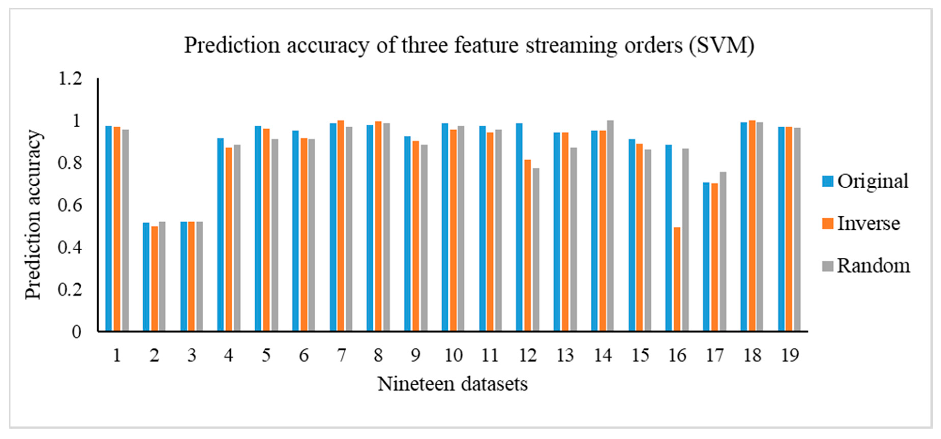
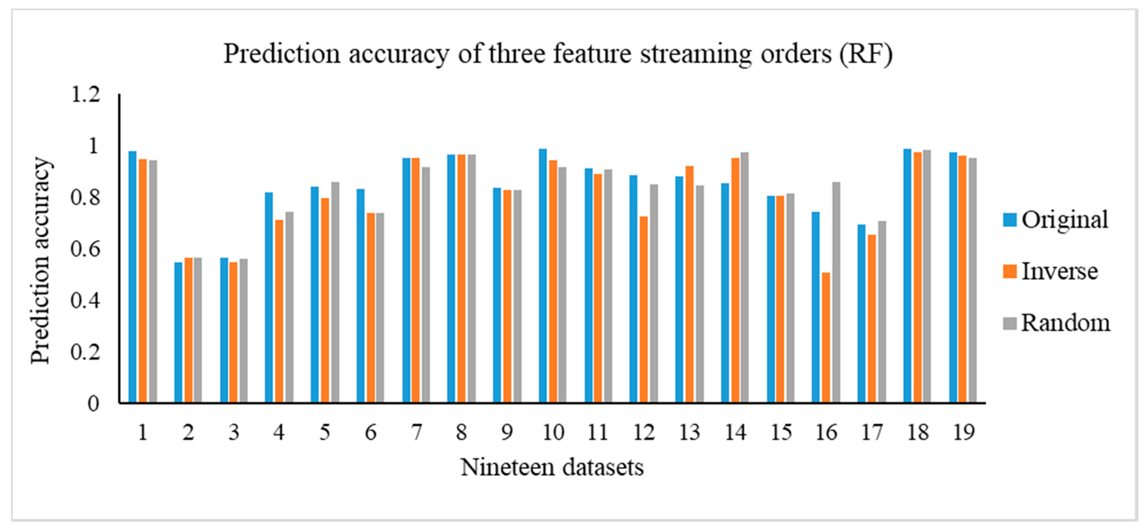
Most of the exiting OSFS methods cannot deal well with the problem of uneven distribution data. In this study, we defined a new $k-\sigma$ neighborhood relation, combining the advantages of k-neighborhood relation and $\delta$ neighborhood relation. Then, we proposed a weighted dependency degree considering the structure of neighborhood covering. Finally, we proposed a new OSFS framework named OSFS-KW, which need not specify any parameters in advance. In addition, this method can also handle the problem of imbalance classes in medical datasets. With three evaluation criteria, this approach can select the optimal feature subset mapping decision attributes. Finally, we used KNN, SVM, and RF as the basic classifiers in conducting the experiments to validate the effectiveness of our method. The results of the Friedman test indicate that a significant difference exists between the OSFS-KW and other neighborhood relations on compactness and running time, but there was no significant difference on the predictive accuracy. Moreover, when comparing with the 11 traditional feature selection methods and five existing OSFS algorithms, the performance of OFS-KW is better than that of the traditional feature selection methods and outperforms that of the state-of-the-art OSFS. However, we only focused on the challenges of medical data and used only medical datasets to verify the validity of our approach. Virtually, our method can be applied into other similar fields, generally. In the future, we will test and evaluate this method using some multidisciplinary datasets.

References

1. Zhou, H.; Wang, J.; Zhang, H. Stochastic multicriteria decision-making approach based on SMAA-ELECTRE with extended gray numbers. Int. Trans. Oper. Res. 2019, 26, 2032–2052. [Google Scholar] [CrossRef]
2. Tian, Z.-P.; Wang, J.; Wang, J.-Q.; Chen, X.-H. Multicriteria decision-making approach based on gray linguistic weighted Bonferroni mean operator. Int. Trans. Oper. Res. 2018, 25, 1635–1658. [Google Scholar] [CrossRef]
3. Tian, Z.-P.; Wang, J.; Wang, J.; Zhang, H.-Y. Simplified Neutrosophic Linguistic Multi-criteria Group Decision-Making Approach to Green Product Development. Group Decis. Negot. 2017, 26, 597–627. [Google Scholar] [CrossRef]
4. Cang, S.; Yu, H. Mutual information based input feature selection for classification problems. Decis. Support Syst. 2012, 54, 691–698. [Google Scholar] [CrossRef]
5. Wang, Z.; Zhang, Y.; Chen, Z.; Yang, H.; Sun, Y.; Kang, J.; Yang, Y.; Liang, X. Application of ReliefF algorithm to selecting feature sets for classification of high resolution remote sensing image. In Proceedings of the 2016 IEEE International Geoscience and Remote Sensing Symposium (IGARSS), Beijing, China, 10–15 July 2016; Institute of Electrical and Electronics Engineers (IEEE): Piscataway, NJ, USA, 2016; pp. 755–758. [Google Scholar]
6. Saqlain, S.M.; Sher, M.; Shah, F.A.; Khan, I.; Ashraf, M.U.; Awais, M.; Ghani, A. Fisher score and Matthews correlation coefficient-based feature subset selection for heart disease diagnosis using support vector machines. Knowl. Inf. Syst. 2018, 58, 139–167. [Google Scholar] [CrossRef]
7. Benabdeslem, K.; Elghazel, H.; Hindawi, M. Ensemble constrained Laplacian score for efficient and robust semi-supervised feature selection. Knowl. Inf. Syst. 2015, 49, 1161–1185. [Google Scholar] [CrossRef]
8. Tibshirani, R. Regression Shrinkage and Selection Via the Lasso. J. R. Stat. Soc. Ser. B (Statal Methodol.) 2011, 73, 273–282. [Google Scholar] [CrossRef]
9. Kumar, V.; Minz, S. Multi-view ensemble learning: An optimal feature set partitioning for high-dimensional data classification. Knowl. Inf. Syst. 2015, 49, 1–59. [Google Scholar] [CrossRef]
10. Wang, J.; Zhao, P.; Hoi, S.C.H.; Jin, R. Online Feature Selection and Its Applications. IEEE Trans. Knowl. Data Eng. 2013, 26, 698–710. [Google Scholar] [CrossRef] [Green Version]
11. Glocer, K.; Eads, D.; Theiler, J. Online feature selection for pixel classification. In Proceedings of the 22nd International Conference on Software Engineering: ICSE 2000, the New Millennium, Limerick, Ireland, 4–11 June 2000; Association for Computing Machinery (ACM): New York, NY, USA, 2005; pp. 249–256. [Google Scholar]
12. Javidi, M.M.; Eskandari, S. Online streaming feature selection: A minimum redundancy, maximum significance approach. Pattern Anal. Appl. 2018, 22, 949–963. [Google Scholar] [CrossRef]
13. Yu, K.; Wu, X.; Ding, W.; Pei, J. Scalable and Accurate Online Feature Selection for Big Data. ACM Trans. Knowl. Discov. Data 2016, 11, 1–39. [Google Scholar] [CrossRef]
14. Eskandari, S.; Javidi, M.M. Online streaming feature selection using rough sets. Int. J. Approx. Reason. 2016, 69, 35–57. [Google Scholar] [CrossRef]
15. Perkins, S.; Theiler, J. Online feature selection using grafting. In Proceedings of the 20th International Conference on Machine Learning (ICML-03), Los Alamos, NM, USA, 21–24 August 2003; pp. 592–599. [Google Scholar]
16. Wu, X.; Yu, K.; Ding, W.; Wang, H.; Zhu, X. Online Feature Selection with Streaming Features. IEEE Trans. Pattern Anal. Mach. Intell. 2012, 35, 1178–1192. [Google Scholar] [CrossRef] [Green Version]
17. Pawlak, Z. Rough sets. Int. J. Comput. Inf. Sci. 1982, 11, 341–356. [Google Scholar] [CrossRef]
18. Yao, Y.; She, Y. Rough set models in multigranulation spaces. Inf. Sci. 2016, 327, 40–56. [Google Scholar] [CrossRef]
19. Javidi, M.M.; Eskandari, S. Streamwise feature selection: A rough set method. Int. J. Mach. Learn. Cybern. 2016, 9, 667–676. [Google Scholar] [CrossRef]
20. Kumar, S.U.; Inbarani, H.H. PSO-based feature selection and neighborhood rough set-based classification for BCI multiclass motor imagery task. Neural Comput. Appl. 2016, 28, 3239–3258. [Google Scholar] [CrossRef]
21. Zhang, J.; Li, T.; Ruan, D.; Liu, D. Neighborhood rough sets for dynamic data mining. Int. J. Intell. Syst. 2012, 27, 317–342. [Google Scholar] [CrossRef]
22. Zhou, P.; Hu, X.-G.; Li, P.; Wu, X. Online streaming feature selection using adapted Neighborhood Rough Set. Inf. Sci. 2019, 481, 258–279. [Google Scholar] [CrossRef]
23. Lin, Y.; Li, J.; Lin, P.; Lin, G.; Chen, J. Feature selection via neighborhood multi-granulation fusion. Knowl. Based Syst. 2014, 67, 162–168. [Google Scholar] [CrossRef]
24. Zhou, P.; Hu, X.; Li, P.; Wu, X. Online feature selection for high-dimensional class-imbalanced data. Knowl. Based Syst. 2017, 136, 187–199. [Google Scholar] [CrossRef]
25. Pawlak, Z. Rough sets and intelligent data analysis. Inf. Sci. 2002, 147, 1–12. [Google Scholar] [CrossRef] [Green Version]
26. Hu, Q.; Yu, D.; Liu, J.; Wu, C. Neighborhood rough set based heterogeneous feature subset selection. Inf. Sci. 2008, 178, 3577–3594. [Google Scholar] [CrossRef]
27. Mac Parthalain, N.; Shen, Q.; Jensen, R. A Distance Measure Approach to Exploring the Rough Set Boundary Region for Attribute Reduction. IEEE Trans. Knowl. Data Eng. 2009, 22, 305–317. [Google Scholar] [CrossRef] [Green Version]
28. Maciá-Pérez, F.; Berna-Martinez, J.V.; Oliva, A.F.; Ortega, M.A.A. Algorithm for the detection of outliers based on the theory of rough sets. Decis. Support Syst. 2015, 75, 63–75. [Google Scholar] [CrossRef] [Green Version]
29. Peng, H.; Long, F.; Ding, C. Feature selection based on mutual information criteria of max-dependency, max-relevance, and min-redundancy. IEEE Trans. Pattern Anal. Mach. Intell. 2005, 27, 1226–1238. [Google Scholar] [CrossRef]
30. Wang, Y.; Klijn, J.G.; Zhang, Y.A.; Sieuwerts, M.; Look, M.P.; Yang, F.; Talantov, D.; Timmermans, M.; Meijer-van Gelder, M.E.; Yu, J. Gene-expression profiles to predict distant metastasis of lymph-node-negative primary breast cancer. Lancet 2005, 365, 671–679. [Google Scholar] [CrossRef]
31. Rosenwald, A.; Wright, G.; Chan, W.C.; Connors, J.M.; Campo, E.; Fisher, R.I.; Gascoyne, R.D.; Müller-Hermelink, H.K.; Smeland, E.B.; Giltnane, J.M.; et al. The Use of Molecular Profiling to Predict Survival after Chemotherapy for Diffuse Large-B-Cell Lymphoma. N. Engl. J. Med. 2002, 346, 1937–1947. [Google Scholar] [CrossRef]
32. Yu, L.; Ding, C.; Loscalzo, S. Stable feature selection via dense feature groups. In Proceedings of the 14th ACM SIGKDD International Conference on Knowledge Discovery and Data Mining (KDD ‘08), Las Vegas, NV, USA, 24–27 August 2008; Association for Computing Machinery (ACM): New York, NY, USA, 2008. [Google Scholar]
33. Yang, K.; Cai, Z.; Li, J.; Lin, G. A stable gene selection in microarray data analysis. BMC Bioinform. 2006, 7, 228. [Google Scholar] [CrossRef] [Green Version]
34. Richardson, A.M. Nonparametric Statistics for Non-Statisticians: A Step-by-Step Approach by Gregory W. Corder, Dale I. Foreman. Int. Stat. Rev. 2010, 78, 451–452. [Google Scholar] [CrossRef]
35. Demšar, J. Statistical comparisons of classifiers over multiple data sets. J. Mach. Learn. Res. 2006, 7, 1–30. [Google Scholar]
36. Gu, Q.; Li, Z.; Han, J. Generalized Fisher Score for Feature Selection. arXiv 2012, arXiv:1202.3725. [Google Scholar]
37. Zhao, Z.; Liu, H. Spectral feature selection for supervised and unsupervised learning. In Proceedings of the 24th International Conference on Real-Time Networks and Systems (RTNS ’16), Brest, France, 19–21 October 2016; Association for Computing Machinery (ACM): New York, NY, USA, 2017; pp. 1151–1157. [Google Scholar]
38. Wasikowski, M.; Chen, X.-W. Combating the Small Sample Class Imbalance Problem Using Feature Selection. IEEE Trans. Knowl. Data Eng. 2009, 22, 1388–1400. [Google Scholar] [CrossRef]
39. Robnik-Šikonja, M.; Kononenko, I. Theoretical and Empirical Analysis of ReliefF and RReliefF. Mach. Learn. 2003, 53, 23–69. [Google Scholar] [CrossRef] [Green Version]
40. Guo, J.; Guo, Y.; Kong, X.; He, R.; Quo, Y. Unsupervised feature selection with ordinal locality. In Proceedings of the 2017 IEEE International Conference on Multimedia and Expo (ICME), Hong Kong, China, 10–14 July 2017; pp. 1213–1218. [Google Scholar]
41. Li, F.; Miao, D.; Pedrycz, W. Granular multi-label feature selection based on mutual information. Pattern Recognit. 2017, 67, 410–423. [Google Scholar] [CrossRef]
42. Roffo, G.; Melzi, S.; Castellani, U.; Vinciarelli, A. Infinite Latent Feature Selection: A Probabilistic Latent Graph-Based Ranking Approach. In Proceedings of the 2017 IEEE International Conference on Computer Vision (ICCV), Venice, Italy, 22–29 October 2017; pp. 1407–1415. [Google Scholar]
43. Fonti, V.; Belitser, E. Feature selection using lasso. VU Amst. Res. Pap. Bus. Anal. 2017, 30, 1–25. [Google Scholar]
44. Yu, L.; Liu, H. Feature selection for high-dimensional data: A fast correlation-based filter solution. In Proceedings of the 20th International Conference on Machine Learning (ICML-03), Washington, DC, USA, 21–24 August 2003; pp. 856–863. [Google Scholar]
45. Chutia, D.; Bhattacharyya, D.K.; Sarma, J.; Raju, P.N.L. An effective ensemble classification framework using random forests and a correlation based feature selection technique. Trans. GIS 2017, 21, 1165–1178. [Google Scholar] [CrossRef]
46. Zhou, J.; Foster, D.P.; Stine, R.A.; Ungar, L.H. Streamwise feature selection. J. Mach. Learn. Res. 2006, 7, 1861–1885. [Google Scholar]
47. Wu, X.; Yu, K.; Wang, H.; Ding, W. Online streaming feature selection. In Proceedings of the 27th International Conference on Machine Learning (ICML-10), Haifa, Israel, 21–24 June 2010; pp. 1159–1166. [Google Scholar]
48. Yu, K.; Ding, W.; Wu, X. LOFS: A library of online streaming feature selection. Knowl. Based Syst. 2016, 113, 1–3. [Google Scholar] [CrossRef] [Green Version]