Word Vector Models Approach to Text Regression of Financial Risk Prediction

Abstract

Linking textual information in finance reports to the stock return volatility provides a perspective on exploring useful insights for risk management. We introduce different kinds of word vector representations in the modeling of textual information: bag-of-words, pre-trained word embeddings, and domain-specific word embeddings. We apply linear and non-linear methods to establish a text regression model for volatility prediction. A large number of collected annually-published financial reports in the period from 1996 to 2013 is used in the experiments. We demonstrate that the domain-specific word vector learned from data not only captures lexical semantics, but also has better performance than the pre-trained word embeddings and traditional bag-of-words model. Our approach significantly outperforms with smaller prediction error in the regression task and obtains a 4%–10% improvement in the ranking task compared to state-of-the-art methods. These improvements suggest that the textual information may provide measurable effects on long-term volatility forecasting. In addition, we also find that the variations and regulatory changes in reports make older reports less relevant for volatility prediction. Our approach opens a new method of research into information economics and can be applied to a wide range of financial-related applications.

1. Introduction

Big data technologies in the financial environment make it more important to explore useful insights for data-driven decision-making and to take advantage of minimizing risks in the financial market. Previously, the analysis of stock return volatility was a common empirical measure of instability and risk of a company based on historical stock prices. Many financial data analyses focused on the stock prices forecasting using time series modeling approaches [1,2,3,4,5]. These works were concerned about the estimation of the parameters, and test economic hypothesis of the fitted model. They believed that the variations of the stock prices could be captured by well-defined market phenomena.

Recently, financial reporting is the collection and presentation of historical overall performance and the shares of the company. Managers are required to discuss several financial risks related to the operations, including credit risk, interest rate risk, and currency risk, in financial reports. Linking textual information of financial reports to the stock return volatility provides an interesting perspective to test market efficiency theory in information economics [6]. Previous studies tended to adopt text mining techniques, such as sentiment analysis and/or bag-of-words models, from the annual financial reports for stock return classification [7,8,9,10,11,12,13]. Sentiment analysis is commonly based on general dictionaries, and/or a finance-specific dictionary proposed by Loughran and McDonald [14] in classifying abnormal stock returns. Instead of analyzing whole reports, they focused on the sentiment lexicon and have yield improved results. Previous studies denote that almost three-fourths of the words identified as negative sentiment in the general domain dictionary, which are typically not considered as negative terms in the financial domain [14,15]. In addition, both positive and negative sentiments are informative, but they do not have symmetric implications of the quantitative information [16]. Measuring positive sentiment in a financial report is challenging because the positive sentiment tends to be ambiguous, where they are often used to convey negative information [16]. On the other hand, those previous works used a classification model for stock price movement prediction, but it is difficult to determine the threshold to separate the continuous values of the risk factors into several classes.

Some works directly mine the financial report via the text regression method for volatility prediction. Kogan et al. (2009) applied a support vector regression (SVR) approach to predict stock return volatilities of companies based on the financial reports [17]. Some works expanded the financial sentiment lexicon using word embedding and the bag-of-words model as features and applied regression and rank-based support vector machine (SVM) model for volatility prediction [18,19,20]. However, those studies focus on partial word-level analyses, which likely yield biased results or explanations because the usage of words in the finance context is usually complicated. Therefore, the goal of our research is applying the word vector models to form the document vector representations for a real-world continuous volatility of stock return prediction. The remainder of this paper is organized as follows: Section 2 formulates the problem and presents a detailed workflow of our approach. Section 3 investigates the predictive power of our approach. Section 4 discusses the contents of the financial reports, the performance of our approach comparing to state-of-the-art methods, the effects of the training data with different historical periods and the correlated words in financial risk. We conclude the contributions and limitations of our approach in Section 5.

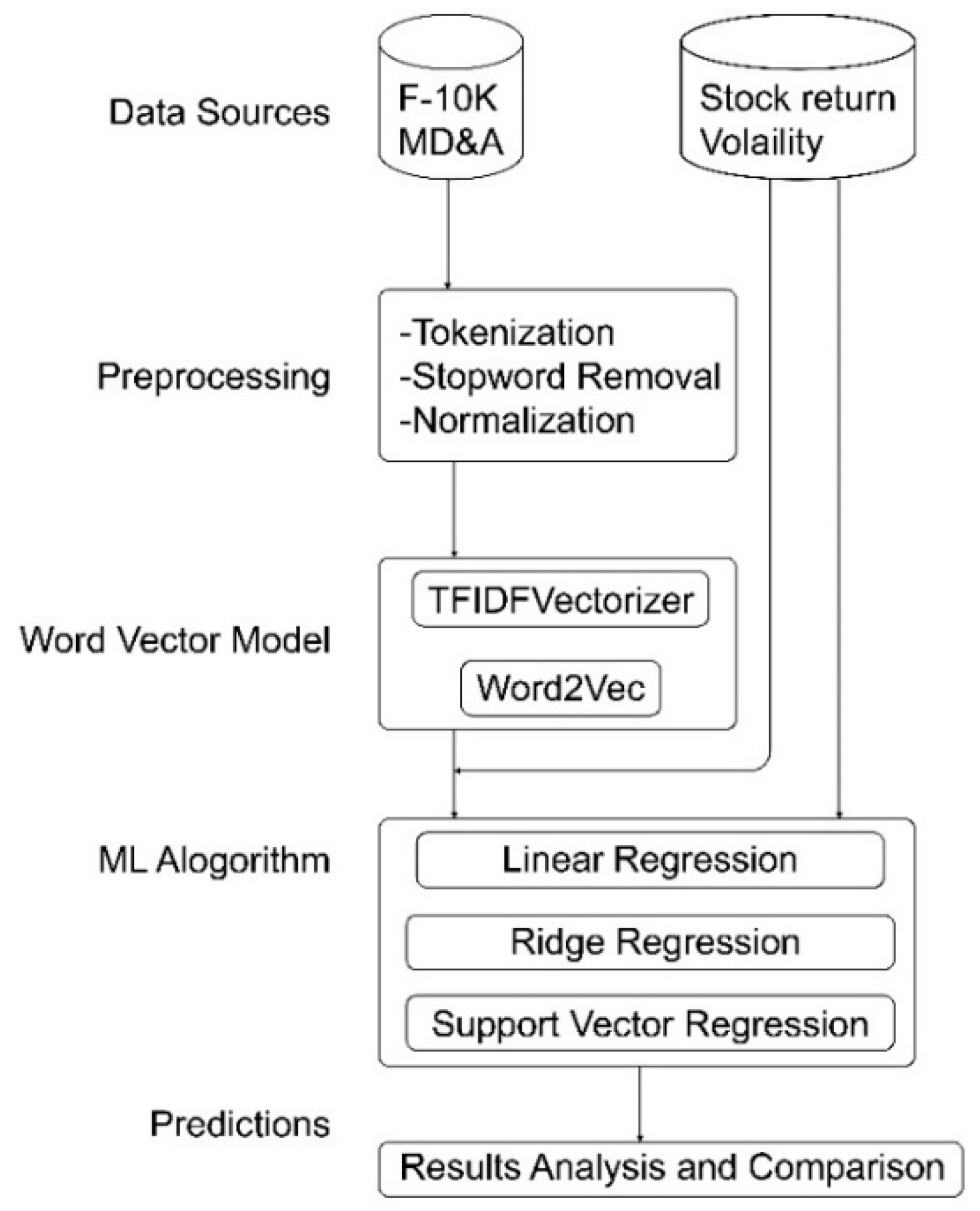
2. Material and Methods

The workflow of our approach is shown in Figure 1. We study textual information in financial report to explain stock return volatility. The preprocessing steps include tokenization, removing stop words, and normalization. The amount of textual data is massive, and we need to represent a format that can be mathematically used to solve the text regression problem. We generate different kinds of word vector representations as a feature set. Then, we apply linear and nonlinear methods to train the text regression model for future stock return volatility prediction.

2.1. Text Preprocessing

We introduce the main steps of text preprocessing: (1) Transformation: it converts all the text to the same case, and removes punctuation. All symbols are replaced with white spaces, except for letters, numbers, and some special symbols, such as “!, ?, ‘, ’”…etc. (2) Tokenization: it separates the document into several sentences and then splits the word tokens. (3) Stop words removal: stop words are words that have no meaning but they are useful in a language to help put sentences together. All English stop words which are as defined in the nltk package were removed [21]. (4) Normalization: for grammatical reasons, words present different forms, but there are sets of various derivationally-related words with similar meanings. It would be useful to reduce various forms to a common base using stemming or lemmatization methods.

2.2. Stock Return Volatility

In finance, volatility is a common empirical measure of the risks and it is interpreted as the standard divergence of the return of a stock over a period, and historical stock return volatilities can be collected from past markets. Prices of stocks fluctuate cause high volatility. High fluctuations in stock prices can possibly increase risk of the future returns. On the other hand, a stock volatility is relatively low when its price remains the same.

Let $R_t=\frac{S_t}{S_{t-1}}-1$ be the net return of a stock between the day $t-1$ and day $t$, where $S_t$ is the stock price at day $t$. The volatility can be measured over the period from day $t-n$ to day $t$ via standard deviation which is defined as Equation (1) [15,17]:

$$volatilit{y}_{\left[t-n,t\right]}=\sqrt{\frac{{\sum }_{i=t-n}^t{\left(R_i-\overline{R}\right)}^2}{n}}$$

(1)

where $\overline{R}$ is the mean of $R_i$ over the period, which is defined as Equation (2):

$$\overline{R}= \frac{{\sum }_{i=t-n}^t{R}_i}{n+1}$$

(2)

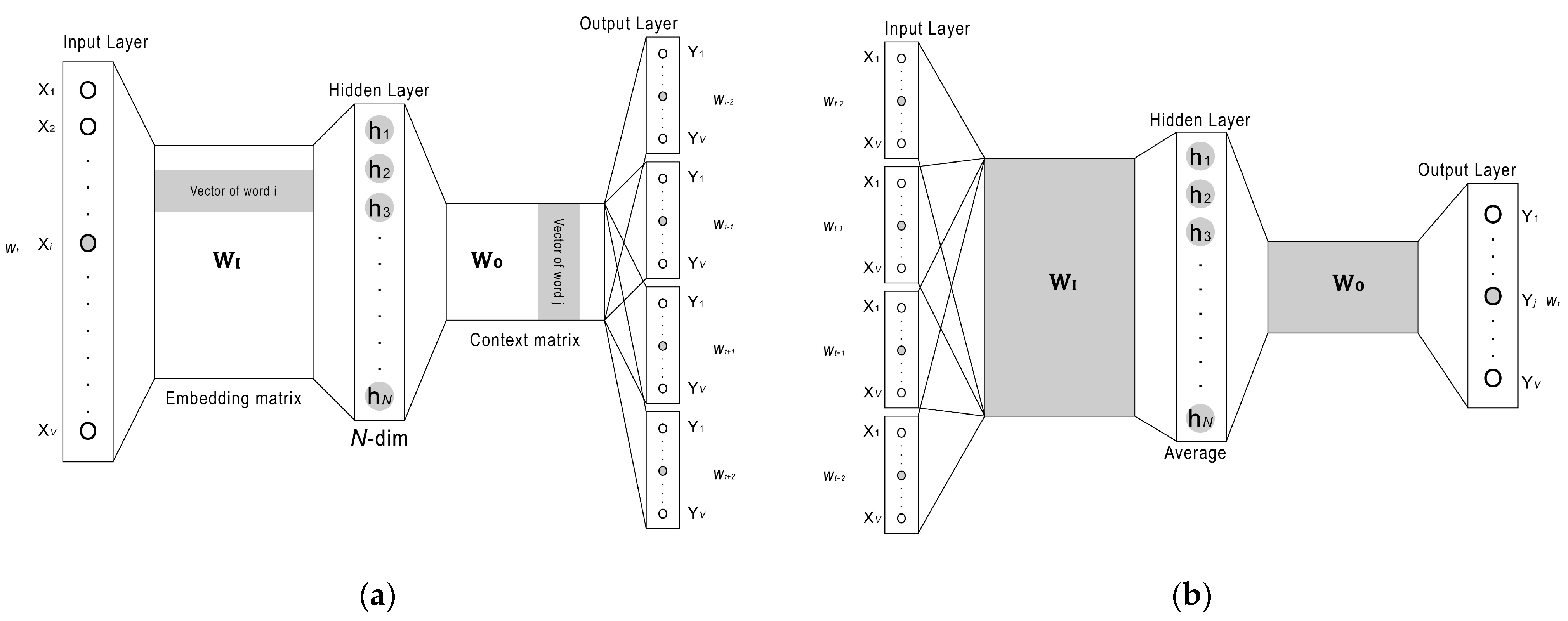
2.3. Word Vector Model Approach

The vector representations of words are commonly used in natural language processing tasks. In the traditional bag-of-words model, term frequency-inverse document frequency, called TF-IDF, is a commonly used weighting technique for information retrieval and text mining. The term frequency (TF) is defined as the number of times that term t occurs in document d, denoted as $t{f}_{t,d}$. For a specific document, it decides how important a word is by looking at how frequently it appears in the document [22]. On the other hand, inverse document frequency (IDF) is based on counting the frequency that a term occurs in a document set, and also provides a higher weight for rare words than common words [23]. A term that rarely occurs in other documents represents that the vocabulary is more representative. It obtains the total number of documents dividing by the number of documents containing the term, and then takes the logarithm of that quotient, as shown by Equation (3):

$$id{f}_{t,D}=\log \frac{\left|D\right|}{\left|\left\{d\in D:t\in d\right\}\right|}$$

(3)

where D denotes the set of the collected documents. The TF-IDF weight of a word token in each document is the product of its TF score and IDF score, as shown by Equation (4). The greater the value of TF-IDF denotes this word as more important, which can provide more information for document representation.

$$w_{t,d,D}=t{f}_{t,d}\times id{f}_{t,D}.$$

(4)

TF-IDF suffers from data sparsity and high dimensionality. To overcome the disadvantage of the bag-of-words model, the continuous vector space of word embedding algorithms, such as word2vec, using neural network techniques are proposed [24,25,26]. In contrast to the traditional bag-of-words model, word2vec considers the order of the words in the sentence and preserves the semantics of words. The aim of word2vec is to build a low dimensional vector of the word from a corpus of text and provides an expressive and efficient representation by considering the contextual of the word.

The structure of word2vec is summarized as follows: an input, a single hidden layer, and an output layer are constructed by a fully-connected neural network for training in Figure 2 [24]. The input layer is set as same as the numbers of the words in the vocabulary. The neurons in the hidden layer are all set with linear function and the size of the hidden layer is set to the dimension of the word embedding which always obtains a lower dimension than those in the input layer. The size of the output layer is the same as that of the input layer. Take as an example, the input document consists of $V$ words and the hidden layer h with $N$ dimensions, the connections between input layer and hidden layer can be represented by matrix $W_I$ of size $V\times N$. In the same way, connections between the hidden layer and the output layer can be represented by matrix $W_O$ of size $N\times V$. The input and output layer in the network is encoded by one-hot-encoding representation where only one variable is set to one and rest of the input lines are set to zero. According to the given input and output vectors, this maximizes the product of the embedding and context metrics for the true samples and minimizes the function for negative examples. The final step of this model is to correct the weights of the matrices $W_I$ and $W_O$ based on the back propagation of the error gradient being similar to the symmetric singular value decomposition (SVD) [24].

Word2vec offers two distinct neural models: continuous bag-of-words (CBOW) and the skip-gram model, which predict words based on their context. These two methods have drawn great attentions and they are the most efficient ways for learning vector representations of words. The aim of the skip-gram model is to predict the surrounding context words w_t−2, w_t−1, w_t+1, w_t+2 with a fixed window-size around given target words w_t, as shown in Figure 2a. The CBOW model predicts the target word by given context words, as shown in Figure 2b. Both of them discover semantic meanings of words by examining statistical co-occurrence patterns of the words within a corpus.

The training processes can learned by a large number of the context-target words set from the text corpus and make the similarity of the hidden word vectors between any two of the co-occurrence words closer to each other. The objective function of the skip-gram model is to estimate the log probability, as shown by Equation (5):

$$\frac{1}{T}{\displaystyle \sum }_{t=1}^T{\displaystyle \sum }_{-C\le j\le C,j\ne 0}\log p\left(w_{t+j}|w_t\right)$$

(5)

where T is the size of the training corpus, and C is the window size determining the span of the center target word $w_t$. $p\left(w_{t+j}|w_t\right)$ is the probability of a context word given the target word. Since the probabilities of the words in the output layer reflects their relationship with other words at the input and the sum of the neuron outputs in the output layer should be one. We apply the softmax function to compute the probability of predicting the output word W_o given the input word vector W_I, as shown by Equation (6):

$$p\left(w_O|w_I\right)=\frac{e^{\left({v_{w_O}^{\prime }}^T{v}_{w_I}\right)}}{{\sum }_{i=1}^N{e}^{\left({v_{w_i}^{\prime }}^T{v}_{w_I}\right)}}$$

(6)

where $v_w$ and $v_w^{\prime }$ are the corresponding vector if the embedding and context matrix w_I and w_O, and N is the number of words in the vocabulary.

In CBOW mode, the input layer corresponds to the context words and the hidden layer corresponds to the projection of the input layer. Assuming multiple context-target words set use the same projection matrix to connect the hidden layer Q times, and the projection matrix dividing by Q in the hidden layer, as shown by Equation (7). The hidden layer is the average of word vectors corresponding to the context-target words as word embedding matrix. The objective function of CBOW model is to estimate the log probability, as shown by Equation (8):

$$h=\frac{1}{Q}W·\left({\displaystyle \sum }_{i=1}^Q{x}_i\right).$$

(7)

$$\frac{1}{T}{\displaystyle \sum }_{t=1}^T\log p\left(w_t|w_{t-C},\dots ,w_{t-1},w_{t+1},\dots ,w_{t+C}\right).$$

(8)

We broaden the textual analysis of financial reports from word level to the document level. Supposing that we have w₁, w₂,…, w_n words in the document, we apply the following representation techniques in order to form document vector:

(1)

TF-IDF. A document vector consists of words with TF-IDF weights, and each unique word is a different dimension in the document-word matrix.

(2)

Avg-Word2vec with pre-trained model. Many studies prefer to use pre-trained models because of the high computation and training time required for large text corpus. Each word has its own vector, and we average the vectors of words by dividing the number of the words appearing in a document.

(3)

Avg-Word2vec trained by our corpus (domain-specific word2vec). Word vectors learned from pre-trained model may not always suitable estimate of semantic similarity among words in target domain. Therefore, we generate domain-specific word2vec model learned from a given collected text corpus, a document vector is also obtained by taking the average of the word vectors appearing in a document.

2.4. Text Regression Problem

Given a collection of the financial reports D = {d1, d2,…, dn} where each di is a p-dimensional vector space related to a company Ci, we try to predict the risk via its stock return volatility vi. We proceed to calculate two observed log-based volatilities: one is twelve months prior to the report ($\log {\left(v\right)}^{-\left(12\right)}$) and the other is twelve months after the report ($\log {\left(v\right)}^{+\left(12\right)}$). The goal is to learn the parameters $\theta$ of both p-dimensional vector and $\log {\left(v\right)}^{-\left(12\right)}$ to predict $\log {\left(v\right)}^{+\left(12\right)}$. The prediction formula can be defined by a text regression function f, as shown by Equation (9):

$$log{\left(v_i\right)}^{+\left(12\right)}= f\left(d_{i },log{\left(v_i\right)}^{-\left(12\right)};\theta \right)$$

(9)

We use linear and nonlinear methods for training this type of regression function. Linear regression is a method of modeling a target based on independent values of the predictors and mostly used for forecasting. We also apply ridge regression, which adds a small squared bias to alleviate collinearity in a model. Support vector regression (SVR) is a popular method for text regression problem in previous studies [15,17] and it is also the reason that we choose SVR as our nonlinear method for training.

2.5. Evaluation Metrics

We used two strategies to evaluate the performance in our experiments, which are the mean squared error (MSE) and two rank correlation metrics: Spearman’s rho [27] and Kendall’s tau [28]. For the regression task, we measure MSE between the predicted and true log-volatilities from a sample of $n$ data points to evaluate the performance. The within-sample MSE is computed, as shown by Equation (10):

$$MSE=\frac{1}{n}{\displaystyle \sum }_{i=1}^n{\left(\log \left({v_i}^{+\left(12\right)}\right)-\log \left({{\widehat{v}}_i}^{+\left(12\right)}\right)\right)}^2.$$

(10)

Given two ranked lists of the companies, one is the ranking list $S=\left\{s_1,s_2,\dots ,s_n\right\}$ based on the true stock return volatility and the other ranking list $P=\left\{p_1,p_2,\dots ,p_n\right\}$ is based on the predicted values generated from the model, respectively. The Spearman’s rho and Kendall’s tau are defined as shown by Equations (11) and (12):

$$Rho=1-\frac{6\sum {\left(s_i-p_i\right)}^2}{n\left(n^2-1\right)}$$

(11)

$$Tau=\frac{\#concordantpairs-\#discordantpairs}{0.5·n·\left(n-1\right)}.$$

(12)

For Kendall’s tau, any pair of observations $\left(s_i,p_i\right)$ and $\left(s_j,p_j\right)$ is concordant if both $s_i>s_j$ and $p_i>p_j$ or if both $s_j>s_i$ and $p_j>p_i$. In contrast, it is discordant pair if $s_i>s_j$ and $p_j>p_i$ or if $s_j>s_i$ and $p_i>p_j$. On the other hand, if $s_i=s_j$ or $p_i=p_j$ denotes neither concordant nor discordant pair.

3. Experiments and Results

A large collection of annually-published financial reports is used as the benchmark in our experiments. The Securities Exchange Commission (SEC) produces public annual financial reports known as “Form 10-K”. The section of the Form 10-K, “Management’s Discussion and Analysis of Financial Conditions and Results of Operations”, is considered in our study. We use the Center for Research in Security Prices (CRSP) US Stocks Database to obtain the stock price return. We collect 40,708 reports published during the period of 1996–2013 with 126,841 unique word tokens in

Table 1. The statistics of the corpus (# denotes the numbers).

Year	# of Documents	# of Unique Terms	Year	# of Documents	# of Unique Terms
1996	1203	18,291	2005	2698	44,303
1997	1705	22,506	2006	2564	44,303
1998	1940	25,487	2007	2495	41,433
1999	1971	26,422	2008	2509	41,924
2000	1884	26,027	2009	2567	42,919
2001	1825	26,602	2010	2439	42,948
2002	2023	32,280	2011	2416	43,404
2003	2866	43,041	2012	2406	42,995
2004	2861	44,642	2013	2336	43,513

. The “# of documents” column in Table 1 shows the number of financial reports each year and the other “# of unique terms” column denotes the numbers of unique terms after tokenization and normalization.

We convert a collection of the documents into a document-word matrix of TF-IDF features with the TfidfTransformer module in the sklearn python package. For the word2vec model, Gensim is a free python library that trains the domain-specific word2vec from raw and unstructured digital texts. We learned the domain-specific word2vec while setting word embeddings to 200, the number of epochs to 100, two surrounding words, and the window-size to eight. On the other hand, we use the pre-trained numberbatch embeddings, which is an ensemble that combines data from ConceptNet [29], word2vec [24], GloVe [30], and OpenSubtitles2016 [31], to produce new embeddings with the performance across many evaluations.

We apply five-fold cross validation to evaluate the performance among different word vector models and regression methods. We use the logarithm of the twelve-month pre-report volatility prior to the financial report (i.e., $\log {\left(v\right)}^{-\left(12\right)}$) to predict the twelve months after the report (i.e., $\log {\left(v\right)}^{+\left(12\right)}$) as a baseline. The lower MSE value get better performance for the regression task, but for the ranking task, higher value of Spearman’s rho or Kendall’s tau measurement are better. The overall performance is shown in

Table 2. Experimental results using different word vector models.

	Linear Regression			Ridge Regression			SVR
Word Vector Representation	MSE	Tau	Rho	MSE	Tau	Rho	MSE	Tau	Rho
Baseline	0.131	0.583	0.777	0.131	0.583	0.777	0.131	0.583	0.777
TF-IDF	>100	0.407	0.581	0.129	0.595	0.791	0.148	0.581	0.784
Pre-trained word2vec	0.131	0.586	0.780	0.125	0.598	0.792	0.131	0.586	0.780
domain-specific word2vec (CBOW)	0.119	0.611	0.802	0.121	0.608	0.799	0.130	0.598	0.782
domain-specific word2vec (Skip-gram)	0.126	0.598	0.790	0.122	0.603	0.795	0.126	0.598	0.790

where the bold number denotes the best result among baseline, and different word vector models each year. The results show that a linear regression based on the TF-IDF model with a sparse document-term matrix is more vulnerable to multicollinearity problems with dependent variables. The larger MSE occurs denoting that it may influence over-fitting in the model. The performance of the domain-specific word2vec is significantly improved with respect to the baseline, and has better performance compared with the pre-trained model and TF-IDF model. We obtain the lowest MSE value of 0.119 and the highest rank value of the Spearman’s rho and Kendall’s tau as 0.802 and 0.611, respectively. Using the pre-trained general word2vec model results in performance comparable to the baseline. The pre-trained word vectors may not be the best fit due to the specific proper nouns in the financial area [29]. We explore the opportunities of using domain-specific word2vec, which can not only present more semantically rich embeddings of the text but also provide better prediction performance.

4. Discussion

In this section, we first analyze the contents of the financial reports. Second, we compare the performance between our approach and state-of-the-art methods based on the text regression technique. Third, we investigate the effect of our approach while considering different historical periods in the training data. Finally, we draw attention to highly weighted words that are associated with volatility.

4.1. Content Analysis of Financial Reports

We calculate the centroid (element-wise mean) avg-word2vec of financial reports in each year and show the L2 distance heatmap for each pair of the years in Figure 3. We observe strong similarities among three ranges of the years: 1996–2000, 2002–2005, and 2007–2013. The Sarbanes-Oxley Act of 2002 enhanced the standards for financial reports to improve the reliability and quality of the reporting. In 2006–2007, the SEC also announced a series of actions and required documents to include management’s assessment of internal controls in the reports. There were substantial changes in reporting which may cause the differences among the centroid avg-word2vec of the financial reports across these three groups. This work is on the analysis of the informativeness of the reports and shows that the content of the reports changes significantly in a cycle of 4–6 years in Figure 3.

4.2. The Performance of Our Approach Comparing with State-of-the-Art Methods

While the above experiments are based on the cross-validation strategy in Section 3, it is reasonable to consider the future volatility prediction based on past data in real-world applications. Therefore, we apply the training data which follows a five-year period preceding the test data in 2001–2006, the same as the previous works [15,17]. Taking as an example, the first training data is from 1996–2000 and the test data is the following year. Then, we drop the oldest year to obtain the next training data from 1997–2001, 1998–2002, and so forth. Both of the previous works applied LOG1P, normalizing word frequencies for TF with a logarithm, for the regression task, and TF-IDF for the ranking task. In the ranking task, they split the stock return volatilities into different risk levels based on the standard deviation of the logarithm of volatilities of stocks and adopt a ranking SVM method for risk level classification. Since the classification-based model may cause more tied ranks, Kendall’s tau has better statistical properties of observing the concordant and discordant pairs.

Table 3. The performance of volatility prediction compared with state-of-the-art methods.

Year	2001		2002		2003		2004		2005		2006
	MSE	Tau	MSE	Tau	MSE	Tau	MSE	Tau	MSE	Tau	MSE	Tau
LOG1P (All words)	0.180	0.622	0.172	0.636	0.172	0.585	0.129	0.593	0.130	0.597	0.143	0.576
LOG1P (sentiment)	0.185	0.633	0.164	0.623	0.158	0.605	0.128	0.590	0.130	0.603	0.140	0.583
Our approach	0.113	0.674	0.102	0.657	0.148	0.679	0.067	0.697	0.066	0.654	0.064	0.651

summarizes the results and our approach yield better performance in both regression and ranking tasks compared with state-of-the-art methods. Our experimental results show that our approach significantly outperforms with smaller MSE and a 4%–10% improvement in the ranking task. Further, the improvements suggest that the financial reporting may provide measurable effects on volatility prediction and also shows the effectiveness of our approach in long-term volatility forecasting.

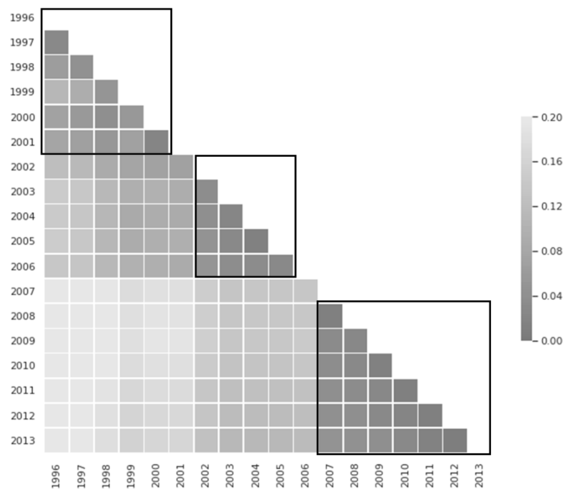
4.3. The Effects of the Training Data with Different Historical Periods

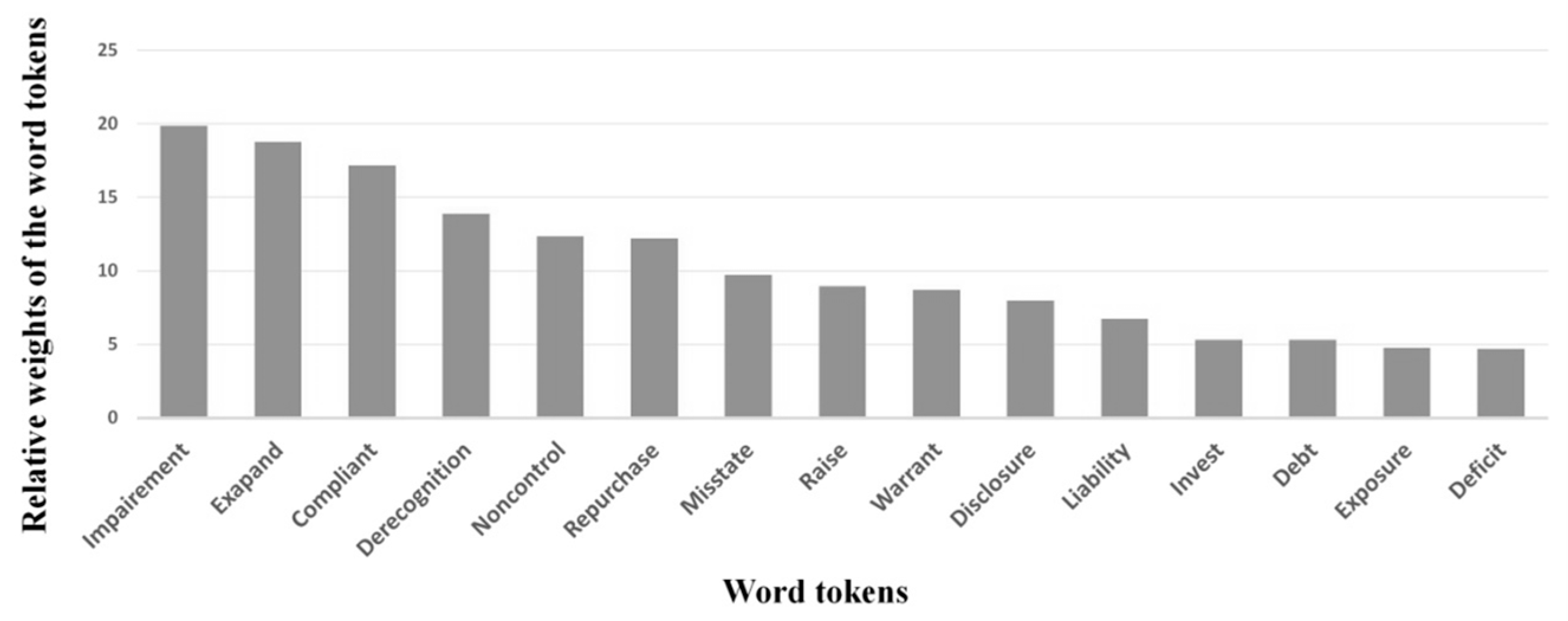
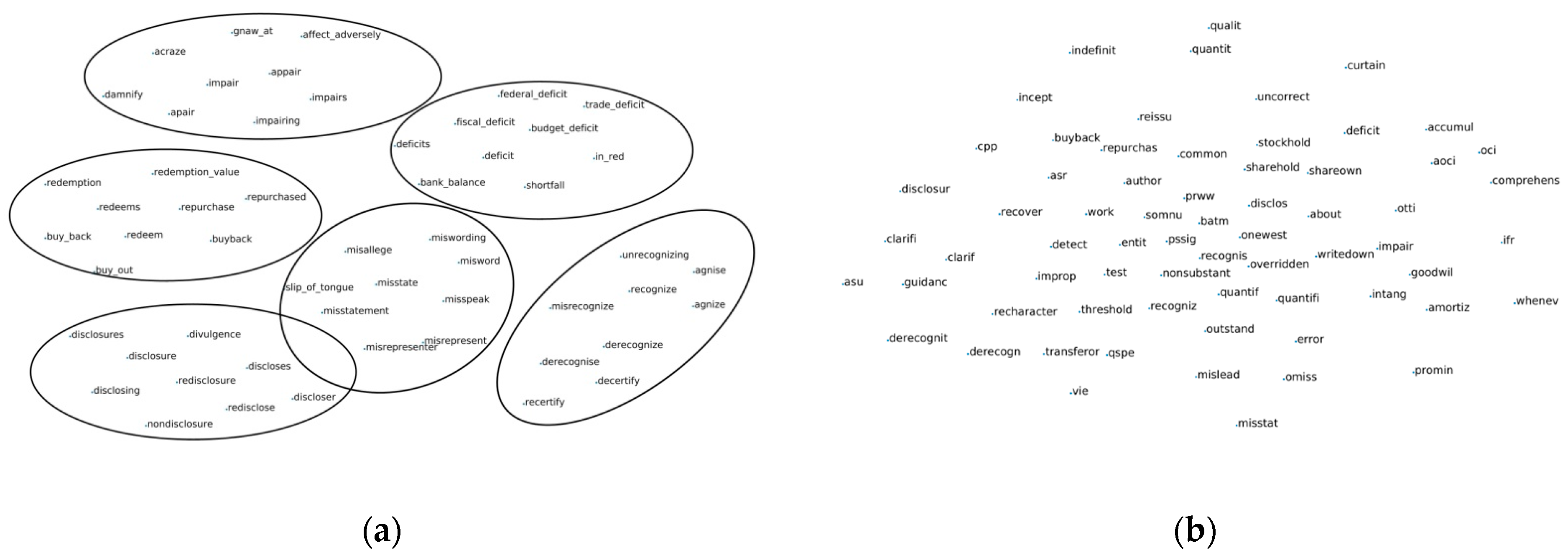
It is well known that the different training data may influence the performance of the method. We apply different training datasets in our model: one of the training datasets with various periods following a five-year period preceding the test data from 2001 to 2006, the same as the setting in Section 4.2, and the other one is trained by the reports published in the fixed period from 1996 to 2000. We observe the performance significantly improving while dropping the oldest reports one-by-one in

Table 4. The performance among the training data with fixed and varying periods.

Year	2001		2002		2003		2004		2005		2006
Training Data	MSE	Tau	MSE	Tau	MSE	Tau	MSE	Tau	MSE	Tau	MSE	Tau
Fixed period	0.113	0.674	0.106	0.657	0.180	0.678	0.118	0.696	0.100	0.652	0.092	0.650
Varying period	0.113	0.674	0.102	0.657	0.148	0.679	0.067	0.697	0.066	0.654	0.064	0.651

. The experimental results denote that the variations in the business cycle and regulatory changes in financial reports make older reports less relevant for future volatility prediction. It also denotes that more informative the report supported, the better prediction performance obtained after the Sarbanes-Oxley Act of 2002. This is consistent with the previous findings [15,17].

The standard assumption in learning process is that the distribution of the training data are similar than that of the test data. Therefore, we use the most coherent financial reports from 2007 to 2013 in Figure 3. We design the experiments by considering the financial reports published in 2011, 2012, and 2013 as the test set and the reports with different periods preceding the test data as the training set (2007–2010, 2007–2011, and 2007–2012, respectively). We show that the performance varies when considering the training data with four, five, or six years in

Table 5. The performance of volatility prediction with different historical periods in 2007–2013.

		Test Data
Year		2011		2012		2013
Training Data	Period	MSE	Tau	MSE	Tau	MSE	Tau
2007–2010	4	0.084	0.607	0.248	0.634	0.192	0.683
2007–2011	5	-	-	0.225	0.646	0.160	0.690
2007–2012	6	-	-	-	-	0.118	0.692

, and the training data with a longer historical period is helpful for volatility prediction in the test set.

4.4. Word Cloud

In addition to the performance comparison, we draw attention to some words that are associated with volatility. We present the highly-weighted words learned by the domain-specific word2vec methods in Figure 4. The word “impairment” occurs while a business suffers depreciation in market value and the market capitalization of the company decreases with a fall in share prices. The term “derecognize” is related to the company having neither transferred nor retained all risks of the asset. The term “repurchase” denotes a company buying back its own shares on the open market. The repurchase boosts the value of the stock and also protects the investor’s benefits for financial statements improvement. The word “misstate” is considered as a key point when the financial statements alters the economic decisions and “disclosure” is the explanation for activities that have significantly influenced the financial results. The misrepresentation of the financial condition through the misstatement of amounts or disclosures in the financial statements must have negatively affected the stock price. The term “deficit” denotes an excess of liabilities or of expenditure over asset and income in finance. This means that higher deficits may lead to higher risk. The textual information in a financial statement reduces information asymmetries in predicting stock return volatility.

We use the keywords “impairment”, “derecognize”, “repurchase”, “misstate”, “deficit”, and “disclosure” as seed words and find the other words that have the higher semantic similarity to the seed word. We display a word cloud of the keywords generated from the general and domain-specific word2vec model in Figure 5a,b, respectively. We place the words into the 2D feature space using the nonlinear dimension reduction technique TSNE [32]. In Figure 5a, there are clearly separated groups and it shows the different semantics of the highly weighted terms from the general domain. However, those words should represent some correlations in the financial domain in Figure 5b. Our findings denote that the pre-trained word embeddings learned from large general dataset, such as Google News, cannot fully capture lexical semantics of the words in specific domain. The distribution of the economic word clouds generated by domain-specific word vectors has intuitive results where words close to each other in semantic meaning are located close to each other.

We calculate the scores between words and highly-weighted terms based on the cosine similarity measurement in

Table 6. Top three similar words among different word vector models.

	Impairment		Derecognize		Repurchase		Misstate
	Word	Sim	Word	Sim	word	Sim	Word	Sim
Pre-trained word2vec	chemofog	0.69	decertify	0.89	repurchased	0.93	misstatement	0.69
	nonaging	0.68	misrecognize	0.60	buyback	0.88	misword	0.68
	impaired	0.67	agnise	0.53	buy_back	0.87	miswording	0.63
domain-specific word2vec	goodwill	0.67	derecognition	0.53	buyback	0.76	uncorrect	0.57
	write-down	0.56	transferor	0.52	reissue	0.45	quantifi	0.54
	intangible	0.53	non-substantial	0.46	onewest	0.45	error	0.45

. Table 6 shows the top three similar terms of the highly-weighted terms. The similar words of the term “repurchase” are synonyms in general domain, but the similar words learned from the domain-specific corpus focus on the effects of the decisions. Take as an example, while the stock price moves back up with repurchase decisions, the company can “reissue” the same number of shares at the new higher price. Companies need to perform a goodwill impairment to realize its impact on the balance sheet, and cash flow statements, and also to report the amount of the write-down on its income statement. Our results show that there are significant connections between word-related activities and volatilities, which can explain the behavior of stock returns. The domain-specific word2vec learned from the annual financial reports not only extracts the synonyms automatically but also obtains the associated terms in understanding the behavior and the impacts on stock price movements.

5. Conclusions

Measuring and managing financial risk and sustainability are critical issues to financial institutions. Linking text information of 10-K reports to the stock return volatility provides an interesting perspective to test market efficiency theory in information economics. We attempt to utilize textual information and market value for volatility prediction among companies through a text regression technique. We outline the domain-specific word vector provides the relevant information to investigate the relationship between textual contents and stock return volatility. The advantage of the domain-specific word vector captures the semantic meaning and the similar words of the economic terms in a systematic way and it avoids the human efforts involved in building dictionaries. Our approach considers a sentence as a sequence of words rather than a bag-of-words model in which the order does not matter and yields better performance compared to state-of-the-art methods in both regression and ranking evaluation methods. The improvements in our approach suggest that the textual information may provide measurable effects on volatility and also demonstrate the effectiveness in long-term volatility forecasting. In addition, we find that the variations and regulatory changes in reports make older reports less relevant for volatility prediction. It is also a challenge to decide which dataset is better to train for predicting volatility in our dataset. There are some limitations of our approach, as follows: we ignore the ordering of the sentences in the document, which limits the information that can be encoded in the sentence vectors. More sophisticated deep learning architectures, including convolutional neural networks and recurrent neural networks, can be used in the future. On the other hand, we simply take the average of the word vector representation of the sentence vector. We can use the weighted average of the word vectors instead of equally weighting the word vectors to pay more attention to significant words. Overall, our approach opens a new method of research into information economics and can be applied to a wide range of financial-related applications.

References

1. Bodyanskiy, Y.; Popov, S. Neural network approach to forecasting of quasiperiodic financial time series. Eur. J. Oper. Res. 2006, 175, 1357–1366. [Google Scholar] [CrossRef]
2. Lee, Y.S.; Tong, L.I. Forecasting time series using a methodology based on autoregressive integrated moving average and genetic programming. Knowl.-Based Syst. 2011, 24, 66–72. [Google Scholar] [CrossRef]
3. Wong, W.K.; Xia, M.; Chu, W. Adaptive neural network model for time-series forecasting. Eur. J. Oper. Res. 2010, 207, 807–816. [Google Scholar] [CrossRef]
4. Hung, J.C. A fuzzy asymmetric Garch model applied to stock markets. Inf. Sci. 2009, 179, 3930–3943. [Google Scholar] [CrossRef]
5. Kim, K.J. Financial time series forecasting using support vector machines. Neurocomputing 2003, 55, 307–319. [Google Scholar] [CrossRef]
6. Pejić Bach, M.; Krstić, Ž.; Seljan, S.; Turulja, L. Text mining for big data analysis in financial sector: A literature review. Sustainability 2019, 11, 1277. [Google Scholar] [CrossRef] [Green Version]
7. Balakrishnan, R.; Qiu, X.Y.; Srinivasan, P. On the predictive ability of narrative disclosures in annual reports. Eur. J. Oper. Res. 2010, 202, 789–801. [Google Scholar] [CrossRef]
8. Nopp, C.; Hanbury, A. Detecting Risks in the Banking System by Sentiment Analysis. In Proceedings of the Conference of Empirical Methods in Natural Language Processing (EMNLP), Lisbon, Portugal, 17–21 September 2015; pp. 591–600. [Google Scholar]
9. Huang, K.W.; Li, Z. A multilabel text classification algorithm for labeling risk factors in sec form 10-K. ACM Trans. Manag. Inf. Syst. 2011, 2, 18. [Google Scholar] [CrossRef]
10. Gidófalvi, G. Using News Articles to Predict Stock Price Movements. Ph.D. Thesis, Department of Computer Science and Engineering, University of California, San Diego, CA, USA, 2001. [Google Scholar]
11. Luss, R.; d’Aspremont, A. Predicting abnormal returns from news using text classification. Quant. Financ. 2009. [Google Scholar] [CrossRef]
12. Lin, M.-C.; Lee, A.J.T.; Kao, R.-T.; Chen, K.-T. Stockprice movement prediction using representative prototypes of financial reports. ACM Trans. Manag. Inf. Syst. 2008, 2. [Google Scholar] [CrossRef]
13. Li, F. The information content of forward looking statements in corporate filings—A naive bayesian machine learning approach. J. Account. Res. 2010, 48, 1049–1102. [Google Scholar] [CrossRef]
14. Loughran, T.; McDonald, B. When is a liability not a liability? Textual analysis, dictionaries, and 10-ks. J. Financ. 2011, 66, 35–65. [Google Scholar] [CrossRef]
15. Tsai, M.F.; Wang, C.J. On the risk prediction and analysis of soft information in finance reports. Eur. J. Oper. Res. 2017, 257, 243–250. [Google Scholar] [CrossRef]
16. Chen, M.P.; Chen, P.F.; Lee, C.C. Asymmetric effects of investor sentiment on industry stock returns: Panel data evidence. Emerg. Mark. Rev. 2013, 14, 35–54. [Google Scholar] [CrossRef]
17. Kogan, S.; Levin, D.; Routledge, B.R.; Sagi, J.S.; Smith, N.A. Predicting risk from financial reports with regression. In Proceedings of the Human Language Technologies: The 2009 Annual Conference of the North American Chapter of the Association for Computational Linguistics (NAACL ’09), Boulder, CO, USA, 1–3 June 2009; pp. 272–280. [Google Scholar]
18. Tsai, M.F.; Wang, C.J. Financial keyword expansion via continuous word vector representations. In Proceedings of the Conference of Empirical Methods in Natural Language Processing (EMNLP), Doha, Qatar, 25–29 October 2014; pp. 1453–1458. [Google Scholar]
19. Wang, C.J.; Tsai, M.F.; Liu, T.; Chang, C.T. Financial sentiment analysis for risk prediction. In Proceedings of the Joint Conference on Natural Language Processing (IJCNLP), Nagoya, Japan, 15 October 2013; pp. 802–808. [Google Scholar]
20. Rekabsaz, N.; Lupu, M.; Baklanov, A.; Hanbury, A.; Duer, A.; Anderson, L. Volatility Prediction using Financial Disclosures Sentiments with Word Embedding-based IR Models. In Proceedings of the Annual Meeting of the Association for Computational Linguistics (ACL 2017), Vancouver, BC, Canada, 30 July 2017; pp. 1712–1721. [Google Scholar]
21. Bird, S.; Klein, E.; Loper, E. Natural Language Processing with Python: Analyzing Text with the Natural Language Toolkit; O’Reilly Media, Inc.: Sebastopol, CA, USA, 2009. [Google Scholar]
22. Jones, S. A Statistical Interpretation of Term Specificity and Its Application in Retrieval. J. Doc. 1972, 28, 11–21. [Google Scholar] [CrossRef]
23. Robertson, S. Understanding Inverse Document Frequency: On theoretical arguments for IDF. J. Doc. 2004, 60, 503–520. [Google Scholar] [CrossRef] [Green Version]
24. Mikolov, T.; Chen, K.; Corrado, G.; Dean, J. Efficient estimation of word representations in vector space. In Proceedings of the International Conference on Learning Representations (ICLR 2013), Scottsdale, AZ, USA, 2–4 May 2013. [Google Scholar]
25. Yoshua, B.; R’ejean, D.; Pascal, V.; Christian, J. A neural probabilistic language model. J. Mach. Learn. Res. 2003, 3, 1137–1155. [Google Scholar]
26. Holger, S. Continuous space language models. Comput. Speech Lang. 2007, 21, 492–518. [Google Scholar]
27. Myers, J.L.; Well, A.; Lorch, R.F. Research Design and Statistical Analysis; Routledge: New York, NY, USA, 2010. [Google Scholar]
28. Kendall, M. A new measure of rank correlation. Biometrika 1938, 30, 81–93. [Google Scholar] [CrossRef]
29. Speer, R.; Chin, J.; Havasi, C. ConceptNet 5.5: An Open Multilingual Graph of General Knowledge. In Proceedings of the AAAI, San Francisco, CA, USA, 4–9 February 2017. [Google Scholar]
30. Pennington, J.; Socher, R.; Manning, C. GloVe: Global Vectors for Word Representation. In Proceedings of the EMNLP, Doha, Qatar, 25–29 October 2014. [Google Scholar]
31. Lison, P.; Tiedemann, J. OpenSubtitles2016: Extracting Large Parallel Corpora from Movie and TV Subtitles. In Proceedings of the LREC, Potolo, Slovenia, 23–28 May 2016. [Google Scholar]
32. Van der Maaten, J.P.; Hinton, G.E. Visualizing High-Dimensional Data Using t-SNE. J. Mach. Learn. Res. 2008, 9, 2579–2605. [Google Scholar]
Figure 1. The workflow of our approach.
Symmetry 12 00089 g001
Figure 2. (a) description of the skip-gram model; and (b) description of the CBOW model.
Symmetry 12 00089 g002
Figure 3. Distance calculation among the centroid word vectors of the years.
Symmetry 12 00089 g003
Figure 4. Highly-weighted terms learned from our model.
Symmetry 12 00089 g004
Figure 5. (a) TSNE 2D position plot of the pre-trained word2vec model; and (b) TSNE 2D position plot of the domain-specific word2vec model.
Symmetry 12 00089 g005