Global Asymptotic Stability and Nonlinear Analysis of the Model of the Square Immunopixels Array Based on Delay Lattice Differential Equations

Abstract

Biosensors and immunosensors show an increasing attractiveness when developing current cheap and fast monitoring and detecting devices. In this work, a model of immunosensor in a class of delayed lattice differential equations is offered and studied. The spatial operator describes symmetric diffusion processes of antigenes between pixels. The main results are devoted to the qualitative research of the model. The conditions of global asymptotic stability, which are constructed with the help of Lyapunov functionals, determine a lower estimate of the time of immune response. Nonlinear analysis of the model is performed with help of a series of numerical characteristics including autocorrelation function, mutual information, embedding, and correlation dimensions, sample entropy, the largest Lyapunov exponents. We consider the influence of both symmetric and unsymmetric diffusion of antigens between pixels on the qualitative behavior of the system. The outcomes are verified with the help of numerical simulation in cases of $4\times 4$- and $16\times 16$- arrays of immunopixels.

1. Introduction

Along with the growing pace of life and the development of civilization, environmental pollution increases, which directly translates into the growing threats to human health and life caused by chemical compounds with genotoxic and cytotoxic properties. Therefore, in addition to detailed analyses performed in specialized laboratories by qualified personnel, the endeavors of technologically advanced societies are increasingly reliant on the development of easy-to-use, cheap and fast devices for monitoring harmful substances in the air, drinking water, soil, or food. Biosensors, which are commonly used in environmental protection [1], medicine [2], the food industry [3] or the defense industry [4] seem to be an excellent solution. In the whole family of biosensors, one can distinguish immunological biosensors (or immunosensors), which are based on the phenomenon of immune response, meaning the binding of antigenes by the corresponding antibodies [5,6]. Given their increasing attractiveness, based on the latest scientific reports, attempts have been made to explore this particular type of sensors in the presented work by showing their specific properties as a dynamical system.

The literature review includes numerous works related to immunosensors, but nothing was found that would bring together selected information on microbiological biosensors based on the phenomenon of luminescence. The following work aims to familiarize the reader with luminescent microbiological biosensors. By learning about them (providing characteristics, mechanisms of action), showing their attractiveness and description of their possible applications, they tried to arouse the interest of the recipient and present the uniqueness of this type of sensors.

In practice, they often develop sensor-like devices that use arrays of pixels [7] and where some diffusion processes are observed. These are the immunosensors that are being studied here.

One of the most important problems arising in immunosensor design is the selection of the parameters of the device giving some properties of its stability. It is characterized by the stable activity of the biosensor matrix components included in the sensible element.

They distinguish two types of stability for biosensors. Namely, self stability is related with activity retention of a sensible device when stored under specific conditions, whereas operational stability means the stable functioning when in use [8].

Using mathematical models described with help of differential equations, we can investigate both types of stability when changing initial conditions for biopixels.

In the works [9,10], the model of immunosensors is offered in the class of differential equations for both square and hexagonal lattices. In [9], the conditions of the local asymptotic stability were proposed, and qualitative behavior was analyzed. However, the questions related to global asymptotic stability for immunosensor’s model on a two-dimensional array of pixels and nonlinear statistics characterizing chaotic behavior remain open.

The objective of this paper is the qualitative investigation of the immunosensor model in the class of differential equations with a delay on a two-dimensional lattice, including global asymptotic stability and a nonlinear analysis of chaotic behavior.

This article is organized as the following. In Section 2, we model the two-dimensional immunopixel array in a class of lattice differential equations with delay. In Section 3, we discuss conditions of the persistence of the model solutions. In Section 4, global asymptotic stability of the equilibrium points for the system is investigated. In Section 5 and Section 6, we show the dynamic features of this system with numerical simulations, including phase portrait, bifurcation diagram, and a series of characteristics of nonlinear dynamics.

2. Modeling Antibody–Antigen Interaction with the Help of Differential Equations on a Two-Dimensional Lattice

Mathematical modeling of arrays of immunopixels is based on lattice differential equations and delayed differential equations [11,12,13,14]. The lattice differential equations are related to the models with the discrete spatial structure [15]. Lattice differential equations arise in many biological problems, such as those described in [16,17,18,19,20,21], where the biological environment is discrete rather than continuous.

A general case can be described as [17]

$$\dot{X_z}=f_z\left({\left\{X_z\right\}}_{z\in \Lambda }\right),z\in \Lambda ,$$

(1)

where $\Lambda \subset {\mathbb{R}}^n$ is a lattice, $X_z$ is the vector in the state space for each $z\in \Lambda$, and $f_z$ is the function of the phase coordinates.

As a rule, they consider $\Lambda ={\mathbb{Z}}^n$, the lattice for integer indices. However, the hexagonal lattice in the plane, and the crystallographic lattices in ${\mathbb{R}}^3$ are also used in some applications.

The problems of population dynamics often use the notion of delay in time. In the case of lattices, they are naturally modeled with help of delayed lattice differential equations [20,22]. The main topics are dealing with the investigation of the stability of traveling wave fronts [17] for the delayed and discretely diffusive models.

The model is constructed with help of the following rate parameters of the populations. We consider an arbitrary biopixel $(i,j)$ located at two-dimensional array (or square lattice) $\Lambda =\{(i,j):i,j=\overline{1,N}\}$. We let $V_{i,j}\left(t\right)$ be the concentration of antigens, and $F_{i,j}\left(t\right)$ be concentration of the antibodies in biopixel $(i,j)$, $i,j=\overline{1,N}$. The biological assumptions resulting in the model are described in [9]. Namely, we use the values of $\beta >0$, constant birthrate for an antigen population, $\gamma >0$, and a probability rate of neutralization of antigens by antibodies, ${\delta }_v>0$, the rate of tending the antigen population to some carrying capacity, $D>0$, the diffusion rate of antibodies from four neighboring pixels $(i-1,j)$, $(i+1,j)$, $(i,j-1)$, $(i,j+1)$, $\Delta >0$, the distance between pixels, ${\mu }_f>0$, a constant birthrate of antibodies, $\eta \gamma$, a probability rate of increase of the density of antibodies as a result of immune response, ${\delta }_f>0$, the rate of tending to some carrying capacity of the antibody population, $\tau >0$, and a constant time delay of an immune response.

The model is based on antibody–antigen competition model with time delay [23,24,25,26] for biopixels’ two-dimensional array, where a spatial operator $\widehat{S}$ was offered in [7] (Supplementary Information, p. 10). The model has the form

$$\begin{array}{cc}\hfill \frac{d{V}_{i,j}\left(t\right)}{dt}& =(\beta -\gamma F_{i,j}(t-\tau )-{\delta }_v{V}_{i,j}(t-\tau ))V_{i,j}\left(t\right)+\widehat{S}\left\{V_{i,j}\right\},\hfill \\ \hfill \frac{d{F}_{i,j}\left(t\right)}{dt}& =(-{\mu }_f+\eta \gamma V_{i,j}(t-\tau )-{\delta }_f{F}_{ij}\left(t\right))F_{i,j}\left(t\right)\hfill \end{array}$$

(2)

with given initial functions

$$\begin{array}{c}{V}_{i,j}\left(t\right)=V_{i,j}^0\left(t\right)\ge 0,F_{i,j}\left(t\right)=F_{i,j}^0\left(t\right)\ge 0,t\in [-\tau ,0),\hfill \\ V_{i,j}\left(0\right),F_{i,j}\left(0\right)>0.\hfill \end{array}$$

(3)

Models (2) and (3) have already been investigated earlier. In [9], the conditions of the local asymptotic stability were obtained. It was shown that they depend on the value of delay $\tau$. In [10], the corresponding model was constructed in the case of a three-dimensional array (or hexagonal lattice) of immunopixels, for which the global asymptotic stability was investigated. In both cases, we evidenced the dependence of phase portraits on $\tau$. We observed complex nonlinear behavior of the model, starting from the stable focus, then switching through Hopf bifurcation to a limit cycle, and through period doublings to chaotic solutions. The chaotic trajectories were evidenced numerically with the help of small deviations of initial conditions and then observing the divergence of trajectories.

The complete analysis of chaotic behavior of trajectories of model (2) have to be executed further with the help of a series of numerical characteristics, which should prove our primary results. Moreover, this research uses the conditions of global asymptotic stability.

Further in Section 5, we present the results of modeling (2). We state that qualitative behavior of the system is affected mostly by the time of immune response $\tau$, diffusion rate $D{\Delta }^{-2}$, and constant n.

The constant $n\le 1$, which is used in the spatial operator $\widehat{S}$, describes the symmetric character of the diffusion between neighboring pixels. Namely, at $n=1$, we have entirely symmetric diffusion (The notion “symmetric diffusion” is introduced similarly to the random symmetric diffusion processes.) and, at $n<1$, we observe unsymmetric diffusion meaning that we do not have the complete exchange by biomass between neighboring pixels.

3. Persistence of the Solutions

Here, we introduce the definition of persistence in accordance with [27], which is adopted for differential equations on a square lattice.

Definition 1.

The lattice system (2) is said to be uniformly persistent if, for all $i,j=\overline{1,N}$, there exist compact regions ${\mathcal{D}}_{i,j}\subset \mathrm{int}{\mathbb{R}}^2$ such that every solution $(V_{i,j}\left(t\right),F_{i,j}\left(t\right))$, $i,j=\overline{1,N}$ of model (2) with the initial conditions (3) finally enters and remains in ${\mathcal{D}}_{i,j}$.

Lemma 1.

Let $(V_{i,j}\left(t\right),F_{i,j}\left(t\right))$, $i,j=\overline{1,N}$ be the solutions of model (2) with initial conditions (3). If

$$\beta \eta \gamma -{\mu }_f{\delta }_v>0,$$

(4)

then

$$\begin{array}{c}\hfill 0<V_{i,j}\left(t\right)\le M_v,\\ \hfill 0<F_{i,j}\left(t\right)\le M_f\end{array}$$

(5)

for some large values of t, where

$$\begin{array}{cc}\hfill M_v& =\frac{\beta }{{\delta }_v}{e}^{\beta \tau },\hfill \\ \hfill M_f& =\frac{1}{{\delta }_f}\left(\eta \gamma M_v-{\mu }_f\right).\hfill \end{array}$$

(6)

Proof. 

In the first step, we prove that there is some large instant of time $T_1$ for which $\widehat{S}\left\{V_{i,j}\left(t\right)\right\}\le 0$, $i,j=\overline{1,N}$, $t>T_1$.

Let us assume the contrary, that is, there is $i^{🞰},j^{🞰}\in \overline{1,N}$, that $\widehat{S}\left\{V_{i,j}\left(t\right)\right\}>0$ at $t>T_1$, which is a contradiction with a balance principle.

Since the solutions of systems (2) and (3) are positive, then

$$\frac{d{V}_{i,j}\left(t\right)}{dt}\le \left(\beta -{\delta }_v{V}_{i,j}(t-\tau )\right)V_{i,j}\left(t\right).$$

(7)

In the second step, we can apply the basic steps of proof of Lemma 3.1 [28] for the nonlattice case.  □

Remark 1.

Conditions of a uniform persistence of system (2) in nonlattice case were obtained in [29]. They resulted in inequality (4) provided that

$$\beta {\delta }_f+{\mu }_f\gamma >0$$

(8)

holds.

4. Stability Problem in Immunosensors

4.1. Steady States

In order to determine the steady states of the model (2), we need to find the solutions of

$$d{V}_{i,j}\left(t\right)/dt=0,d{F}_{i,j}\left(t\right)/dt=0,i,j=\overline{1,N}.$$

(9)

Hence, as it was evidenced in [9], we differ the following cases, when we have the nonnegative solutions of Equation (9). Namely, they are antigen-free steady state ${\mathcal{E}}_{i,j}^0\equiv \left(0,0\right)$, $i,j=\overline{1,N}$, the endemic steady state ${\mathcal{E}}_{i,j}^{*}\equiv \left(V_{i,j}^{*},F_{i,j}^{*}\right)$, $i,j=\overline{1,N}$ as a solution of the algebraic system:

$$\begin{array}{c}\left(\beta -\gamma F_{i,j}^{*}-{\delta }_v{V}_{i,j}^{*}\right)V_{i,j}^{*}+\widehat{S}\left\{V_{i,j}^{*}\right\}=0,\hfill \\ \left(-{\mu }_f+\eta \gamma V_{i,j}^{*}-{\delta }_f{F}_{i,j}^{*}\right)F_{i,j}^{*}=0,i,j=\overline{1,N}.\hfill \end{array}$$

(10)

When considering the solutions $\left(V_{i,j}^{*},F_{i,j}^{*}\right)$ of Equation (10), we can obtain an identical endemic state for all pixels

$$V_{i,j}^{*}=\frac{\beta {\delta }_f+\gamma {\mu }_f}{{\delta }_v{\delta }_f+\eta {\gamma }^2},F_{i,j}^{*}=\frac{\eta \gamma \beta -{\delta }_v{\mu }_f}{{\delta }_v{\delta }_f+\eta {\gamma }^2},$$

(11)

provided that $\eta \gamma \beta >{\delta }_v{\mu }_f$ and nonidentical endemic state for pixels in a general case (if diffusion $D>0$).

4.2. Global Asymptotic Stability

Here, we derive the sufficient conditions of the global asymptotic stability of the endemic steady state ${\mathcal{E}}_{i,j}^{*}=\left(V_{i,j}^{*},F_{i,j}^{*}\right)$, $i,j=\overline{1,N}$.

Theorem 1.

Assume that:

$${\alpha }_1:=\underset{i,j=\overline{1,N}}{max}\left[-{\delta }_v{V}_{i,j}^{🞰}(1-{\delta }_v{M}_v\tau )+\eta \gamma V_{i,j}^{🞰}+\frac{|\widehat{S}\left\{V_{i,j}^{🞰}\right\}|}{V_{i,j}^{🞰}}({\delta }_v{M}_v\tau +1)\right]<0$$

and

$${\alpha }_2:=\underset{i,j=\overline{1,N}}{max}\left[\gamma F_{i,j}^{🞰}(1+{\delta }_v{M}_v\tau )-{\delta }_f{F}_{i,j}^{🞰}\right]<0.$$

Then, the positive equilibrium ${\mathcal{E}}_{i,j}^{🞰}=\left(V_{i,j}^{🞰},F_{i,j}^{🞰}\right)$, $i,j=\overline{1,N}$ of system (2) is globally asymptotically stable.

Proof. 

Let us change the variables

$$x_{i,j}\left(t\right)=log\left(\frac{V_{i,j}\left(t\right)}{V_{i,j}^{*}}\right),y_{i,j}\left(t\right)=log\left(\frac{F_{i,j}\left(t\right)}{F_{i,j}^{*}}\right),i,j=\overline{1,N}.$$

(12)

Herefrom,

$$V_{i,j}\left(t\right)=V_{i,j}^{*}{e}^{x_{i,j}\left(t\right)},F_{i,j}\left(t\right)=F_{i,j}^{*}{e}^{y_{i,j}\left(t\right)}.$$

(13)

Substituting Equation (13) into model (2), we get

$$\begin{array}{cc}\hfill V_{i,j}^{*}{e}^{x_{i,j}\left(t\right)}\frac{d{x}_{i,j}\left(t\right)}{dt}& =\left(\beta -\gamma F_{i,j}^{*}{e}^{y_{i,j}(t-\tau )}-{\delta }_v{V}_{i,j}^{*}{e}^{x_{i,j}(t-\tau )}\right)V_{i,j}^{*}{e}^{x_{i,j}\left(t\right)}+\widehat{S}\left\{V_{i,j}\left(t\right)\right\},\hfill \\ \hfill F_{i,j}^{*}{e}^{y_{i,j}\left(t\right)}\frac{d{y}_{i,j}\left(t\right)}{dt}& =\left(-{\mu }_f+\eta \gamma V_{i,j}^{*}{e}^{x_{i,j}(t-\tau )}-{\delta }_f{F}_{i,j}^{*}{e}^{y_{i,j}\left(t\right)}\right)F_{i,j}^{*}{e}^{y_{i,j}\left(t\right)}.\hfill \end{array}$$

(14)

It yields

$$\begin{array}{cc}\hfill \frac{d{x}_{i,j}\left(t\right)}{dt}& =\beta -\gamma F_{i,j}^{*}{e}^{y_{i,j}(t-\tau )}-{\delta }_v{V}_{i,j}^{*}{e}^{x_{i,j}(t-\tau )}+V_{i,j}^{-1}\left(t\right)\widehat{S}\left\{V_{i,j}\left(t\right)\right\},\hfill \\ \hfill \frac{d{y}_{i,j}\left(t\right)}{dt}& =-{\mu }_f+\eta \gamma V_{i,j}^{*}{e}^{x_{i,j}(t-\tau )}-{\delta }_f{F}_{i,j}^{*}{e}^{y_{i,j}\left(t\right)}.\hfill \end{array}$$

(15)

Since

$$\beta =\gamma F_{i,j}^{*}+{\delta }_v{V}_{i,j}^{*}-\frac{\widehat{S}\left\{V_{i,j}^{*}\right\}}{V_{i,j}^{*}},{\mu }_f=\eta \gamma V_{i,j}^{*}-{\delta }_f{F}_{i,j}^{*},$$

(16)

then

$$\begin{array}{cc}\hfill \frac{d{x}_{i,j}\left(t\right)}{dt}& =-\gamma F_{i,j}^{*}\left[e^{y_{i,j}(t-\tau )}-1\right]-{\delta }_v{V}_{i,j}^{*}\left[e^{x_{i,j}(t-\tau )}-1\right]\hfill \\ & +V_{i,j}^{-1}\left(t\right)\widehat{S}\left\{V_{i,j}^{*}{e}^{x_{i,j}\left(t\right)}\right\}-\frac{\widehat{S}\left\{V_{i,j}^{*}\right\}}{V_{i,j}^{*}},\hfill \\ \hfill \frac{d{y}_{i,j}\left(t\right)}{dt}& =-{\mu }_f+\eta \gamma V_{i,j}^{*}{e}^{x_{i,j}(t-\tau )}-{\delta }_f{F}_{i,j}^{*}{e}^{y_{i,j}\left(t\right)}.\hfill \end{array}$$

(17)

Let $\tilde{S}\left\{x_{i,j}\left(t\right)\right\}=V_{i,j}^{-1}\left(t\right)\widehat{S}\left\{V_{i,j}^{*}{e}^{x_{i,j}\left(t\right)}\right\}-\frac{\widehat{S}\left\{V_{i,j}^{*}\right\}}{V_{i,j}^{*}}.$

Rewrite the first equation as

$$\begin{array}{cc}\hfill \frac{d{x}_{i,j}\left(t\right)}{dt}& =-{\delta }_v{V}_{i,j}^{*}\left[e^{x_{i,j}\left(t\right)}-1\right]-\gamma F_{i,j}^{*}\left[e^{y_{i,j}(t-\tau )}-1\right]\hfill \\ & +{\delta }_v{V}_{i,j}^{*}\left[e^{x_{i,j}\left(t\right)}-e^{x_{i,j}(t-\tau )}\right]+\tilde{S}\left\{x_{i,j}\left(t\right)\right\}=-{\delta }_v{V}_{i,j}^{*}\left[e^{x_{i,j}\left(t\right)}-1\right]\hfill \\ & -\gamma F_{i,j}^{*}\left[e^{y_{i,j}(t-\tau )}-1\right]+{\delta }_v{V}_{i,j}^{*}{\int }_{t-\tau }^t{e}^{x_{i,j}\left(s\right)}\frac{d{x}_{i,j}\left(s\right)}{ds}ds+\tilde{S}\left\{x_{i,j}\left(t\right)\right\}\hfill \\ & =-{\delta }_v{V}_{i,j}^{*}\left[e^{x_{i,j}\left(t\right)}-1\right]-\gamma F_{i,j}^{*}\left[e^{y_{i,j}(t-\tau )}-1\right]\hfill \\ & +{\delta }_v{V}_{i,j}^{*}{\int }_{t-\tau }^t{e}^{x_{i,j}\left(s\right)}\left\{-\gamma F_{i,j}^{*}\left[e^{y_{i,j}(s-\tau )}-1\right]-{\delta }_v{V}_{i,j}^{*}\left[e^{x_{i,j}(s-\tau )}-1\right]+\tilde{S}\left\{x_{i,j}\left(s\right)\right\}\right\}ds\hfill \\ & +\tilde{S}\left\{x_{i,j}\left(t\right)\right\}.\hfill \end{array}$$

(18)

For arbitrary pixel $(i,j)$, $i,j=\overline{1,N}$, consider Lyapunov functionals

$$G_{i,j,1,1}\left(t\right)=\left|x_{i,j}\left(t\right)\right|.$$

Then, we can estimate the right-upper derivative along Equation (18) in the following way:

$$\begin{array}{cc}\hfill \frac{d{G}_{i,j,1,1}\left(t\right)}{dt}& \le -{\delta }_v{V}_{i,j}^{*}|e^{x_{i,j}\left(t\right)}-1|+\gamma F_{i,j}^{*}\left|e^{y_{i,j}(t-\tau )}-1\right|\hfill \\ & +\delta V_{i,j}^{*}{\int }_{t-\tau }^t\left[\gamma F_{i,j}^{*}|e^{y_{i,j}(s-\tau )}-1|+{\delta }_v{V}_{i,j}^{*}|e^{x_{i,j}(s-\tau )}-1|+|\tilde{S}\left\{x_{i,j}\left(s\right)\right\}|\right]ds\hfill \\ & +|\tilde{S}\left\{x_{i,j}\left(t\right)\right\}|.\hfill \end{array}$$

(19)

Since Lemma 1 holds, then there exists a $T_0\ge 0$ such that $V\left(t\right)\le M_v$ for $t\ge T_0$ and, hence, for $t\ge T=T_0+\tau$,

$$\begin{array}{cc}\hfill \frac{d{G}_{i,j,1,1}\left(t\right)}{dt}& \le -{\delta }_v{V}_{i,j}^{*}|e^{x_{i,j}\left(t\right)}-1|+\gamma F_{i,j}^{*}\left|e^{y_{i,j}(t-\tau )}-1\right|\hfill \\ & +{\delta }_v{M}_v[\gamma F_{i,j}^{*}{\int }_{t-\tau }^t|e^{y_{i,j}(s-\tau )}-1|ds+{\delta }_v{V}_{i,j}^{*}{\int }_{t-\tau }^t|e^{x_{i,j}(s-\tau )}-1|ds\hfill \\ & +{\int }_{t-\tau }^t|\tilde{S}\left\{x_{i,j}\left(s\right)\right\}|ds]+\left|\tilde{S}\left\{x_{i,j}\left(t\right)\right\}\right|.\hfill \end{array}$$

Next, let

$$\begin{array}{cc}\hfill G_{i,j,1,2}\left(t\right)& ={\delta }_v{M}_v\left[\gamma F_{i,j}^{*}{\int }_{t-\tau }^t{\int }_{\xi }^t|e^{y_{i,j}(s-\tau )}-1|dsd\xi +{\delta }_v{V}_{i,j}^{*}{\int }_{t-\tau }^t{\int }_{\xi }^t|e^{x_{i,j}(s-\tau )}-1|dsd\xi \right]\hfill \\ & +{\delta }_v{M}_v\tau \left[\gamma F_{i,j}^{*}{\int }_{t-\tau }^t|e^{y_{i,j}\left(s\right)}-1|ds+{\delta }_v{V}_{i,j}^{*}{\int }_{t-\tau }^t|e^{x_{i,j}\left(s\right)}-1|ds\right],\hfill \end{array}$$

$$G_{i,j,1,3}\left(t\right)=\gamma F_{i,j}^{*}{\int }_{t-\tau }^t|e^{y_{i,j}\left(s\right)}-1|ds.$$

Then, we have at $t\ge T$

$$\begin{array}{cc}\hfill \frac{d{G}_{i,j,1}\left(t\right)}{dt}& =\frac{d\left(G_{i,j,1,1}\left(t\right)+G_{i,j,1,2}\left(t\right)+G_{i,j,1,3}\left(t\right)\right)}{dt}\hfill \\ & \le -{\delta }_v{V}_{i,j}^{*}|e^{x_{i,j}\left(t\right)}-1|+\gamma F_{i,j}^{*}\left|e^{y_{i,j}(t-\tau )}-1\right|\hfill \\ & +{\delta }_v{M}_v[\gamma F_{i,j}^{*}{\int }_{t-\tau }^t|e^{y_{i,j}(s-\tau )}-1|ds+{\delta }_v{V}_{i,j}^{*}{\int }_{t-\tau }^t|e^{x_{i,j}(s-\tau )}-1|ds\hfill \\ & +{\int }_{t-\tau }^t|\tilde{S}\left\{x_{i,j}\left(s\right)\right\}|ds]+\left|\tilde{S}\left\{x_{i,j}\left(t\right)\right\}\right|\hfill \\ & +{\delta }_v{M}_v[-\gamma F_{i,j}^{*}{\int }_{t-\tau }^t|e^{y_{i,j}(s-\tau )}-1|ds+\gamma F_{i,j}^{*}\tau \left|e^{y_{i,j}(t-\tau )}-1\right|\hfill \\ & -{\delta }_v{V}_{i,j}^{*}{\int }_{t-\tau }^t|e^{x_{i,j}(s-\tau )}-1|ds+{\delta }_v{V}_{i,j}^{*}\tau \left|e^{x_{i,j}(t-\tau )}-1\right|]\hfill \\ & +{\delta }_v{M}_v\tau [\gamma F_{i,j}^{*}\left(|e^{y_{i,j}\left(t\right)}-1|-|e^{y_{i,j}(t-\tau )}-1|\right)\hfill \\ & +{\delta }_v{V}_{i,j}^{*}\left(|e^{x_{i,j}\left(t\right)}-1|-|e^{x_{i,j}(t-\tau )}-1|\right)]\hfill \\ & +\gamma F_{i,j}^{*}\left[|e^{y_{i,j}\left(t\right)}-1|-|e^{y_{i,j}(t-\tau )}-1|\right]\hfill \\ & =-{\delta }_v{V}_{i,j}^{*}(1-{\delta }_v{M}_v\tau )|e^{x_{i,j}\left(t\right)}-1|+\gamma F_{i,j}^{*}(1+{\delta }_v{M}_v\tau )\left|e^{y_{i,j}\left(t\right)}-1\right|\hfill \\ & +{\delta }_v{M}_v{\int }_{t-\tau }^t|\tilde{S}\left\{x_{i,j}\left(s\right)\right\}|ds+\left|\tilde{S}\left\{x_{i,j}\left(t\right)\right\}\right|.\hfill \end{array}$$

Rewrite the second Equation (17) as

$$\begin{array}{c}\hfill \frac{d{y}_{i,j}\left(t\right)}{dt}=\eta \gamma V_{i,j}^{🞰}\left[e^{x_{i,j}(t-\tau )}-1\right]-{\delta }_f{F}_{i,j}^{🞰}\left[e^{y_{i,j}\left(t\right)}-1\right].\end{array}$$

(20)

We introduce Lyapunov functional for any pixel $(i,j)$, $i,j=\overline{1,N}$

$$G_{i,j,2}\left(t\right)=\left|y_{i,j}\left(t\right)\right|+\eta \gamma V_{i,j}^{🞰}{\int }_{t-\tau }^t|e^{x_{i,j}\left(s\right)}-1|ds.$$

Hence, we estimate the right-upper derivative along Equation (20) in the following way:

$$\begin{array}{cc}\hfill \frac{d{G}_{i,j,2}\left(t\right)}{dt}& \le \eta \gamma V_{i,j}^{🞰}|e^{x_{i,j}(t-\tau )}-1|-{\delta }_f{F}_{i,j}^{🞰}\left|e^{y_{i,j}\left(t\right)}-1\right|\hfill \\ & +\eta \gamma V_{i,j}^{🞰}\left[|e^{x_{i,j}\left(t\right)}-1|-|e^{x_{i,j}(t-\tau )}-1|\right]\hfill \\ & =\eta \gamma V_{i,j}^{🞰}|e^{x_{i,j}\left(t\right)}-1|-{\delta }_f{F}_{i,j}^{🞰}\left|e^{y_{i,j}\left(t\right)}-1\right|.\hfill \end{array}$$

(21)

Let us introduce Lyapunov functional $G_{i,j}\left(t\right)=G_{i,j,1}\left(t\right)+G_{i,j,2}\left(t\right)$. Then,

$$\begin{array}{cc}\hfill \frac{d{G}_{i,j}\left(t\right)}{dt}& \le \left[-{\delta }_v{V}_{i,j}^{🞰}(1-{\delta }_v{M}_v\tau )+\eta \gamma V_{i,j}^{🞰}\right]\left|e^{x_{i,j}\left(t\right)}-1\right|\hfill \\ & +\left[\gamma F_{i,j}^{🞰}(1+{\delta }_v{M}_v\tau )-{\delta }_f{F}_{i,j}^{🞰}\right]\left|e^{y_{i,j}\left(t\right)}-1\right|\hfill \\ & +{\delta }_v{M}_v{\int }_{t-\tau }^t|\tilde{S}\left\{x_{i,j}\left(s\right)\right\}|ds+\left|\tilde{S}\left\{x_{i,j}\left(t\right)\right\}\right|.\hfill \end{array}$$

(22)

We rewrite

$$\begin{array}{cc}\hfill \tilde{S}\left\{x_{i,j}\left(t\right)\right\}& =\frac{\widehat{S}\left\{V_{i,j}\left(t\right)\right\}}{V_{i,j}\left(t\right)}-\frac{\widehat{S}\left\{V_{i,j}^{🞰}\right\}}{V_{i,j}^{🞰}}\hfill \\ & =\left[\frac{\widehat{S}\left\{V_{i,j}\left(t\right)\right\}}{V_{i,j}\left(t\right)}-\frac{\widehat{S}\left\{V_{i,j}\left(t\right)\right\}}{V_{i,j}^{🞰}}\right]+\left[\frac{\widehat{S}\left\{V_{i,j}\left(t\right)\right\}}{V_{i,j}^{🞰}}-\frac{\widehat{S}\left\{V_{i,j}🞰\right\}}{V_{i,j}^{🞰}}\right]\hfill \\ & =\frac{\widehat{S}\left\{V_{i,j}\left(t\right)\right\}}{V_{i,j}\left(t\right)}\left(1-e^{x_{i,j}\left(t\right)}\right)+\left[\frac{\widehat{S}\left\{V_{i,j}\left(t\right)\right\}}{V_{i,j}^{🞰}}-\frac{\widehat{S}\left\{V_{i,j}🞰\right\}}{V_{i,j}^{🞰}}\right].\hfill \end{array}$$

Taking into account that $V_{i,j}^{🞰}$ is steady state, we have that, for any small $ϵ>0$, some instant of time $T_1\left(ϵ\right)$ exists that

$$\tilde{S}\left\{x_{i,j}\left(t\right)\right\}\le \frac{\widehat{S}\left\{V_{i,j}^{🞰}\right\}}{V_{i,j}^{🞰}}\left(1-e^{x_{i,j}\left(t\right)}\right)+ϵ.$$

(23)

Furthermore, we consider $t\ge max\left\{T_0,T_1\left(ϵ\right)\right\}$ and omit $ϵ$ in Equation (23).

It holds that

$$\begin{array}{cc}\hfill \frac{d{G}_{i,j}\left(t\right)}{dt}& \le \left[-{\delta }_v{V}_{i,j}^{🞰}(1-{\delta }_v{M}_v\tau )+\eta \gamma V_{i,j}^{🞰}+\frac{|\widehat{S}\left\{V_{i,j}^{🞰}\right\}|}{V_{i,j}^{🞰}}({\delta }_v{M}_v\tau +1)\right]\left|e^{x_{i,j}\left(t\right)}-1\right|\hfill \\ & +\left[\gamma F_{i,j}^{🞰}(1+{\delta }_v{M}_v\tau )-{\delta }_f{F}_{i,j}^{🞰}\right]\left|e^{y_{i,j}\left(t\right)}-1\right|.\hfill \end{array}$$

Let $G\left(t\right)={\sum }_{i,j=1}^N{G}_{i,j}\left(t\right)$. Estimating the derivative of $G\left(t\right)$ along Equation (20), we get

$$\frac{dG\left(t\right)}{dt}\le {\alpha }_1\sum _{i,j=1}^N|e^{x_{i,j}\left(t\right)}-1|+{\alpha }_2\sum _{i,j=1}^N|e^{y_{i,j}\left(t\right)}-1|\le 0.$$

 □

Corollary 1.

Let the conditions of Theorem 1 hold. Then, we can state that the endemic steady state ${\mathcal{E}}_{i,j}^{🞰}=\left(V_{i,j}^{🞰},F_{i,j}^{🞰}\right)$, $i,j=\overline{1,N}$ of system (2) is globally asymptotically stable at $\tau <min\left\{{\tau }_1,{\tau }_2\right\}$. Here,

$$\begin{array}{cc}\hfill {\tau }_1& :=\underset{i,j=\overline{1,N}}{min}\left\{\frac{{\delta }_v{V}_{i,j}^{🞰}-\eta \gamma V_{i,j}^{🞰}-\frac{|\widehat{S}\left\{V_{i,j}^{🞰}\right\}|}{V_{i,j}^{🞰}}}{{\delta }_v^2{V}_{i,j}^{🞰}{M}_v+\frac{|\widehat{S}\left\{V_{i,j}^{🞰}\right\}|}{V_{i,j}^{🞰}}{\delta }_v{M}_v}\right\},\hfill \\ \hfill {\tau }_2& :=\frac{{\delta }_f-\gamma }{\gamma {\delta }_v{M}_v}.\hfill \end{array}$$

Remark 2.

Conditions of global asymptotic stability of the endemic steady state ${\mathcal{E}}_{i,j}^{🞰}=\left(V_{i,j}^{🞰},F_{i,j}^{🞰}\right)$, $i,j=\overline{1,N}$ of system (2) are determined by the diffusion rate D, distance between pixels Δ and constant of diffusion unsymmetricity n.

Remark 3.

Assumptions of Theorem 1 can be simply interpreted in the context of parameters of population colonies within immunopixels. Namely, analyzing the assumptions reformulated in Corollary 1, due to the second inequality, we see that the bigger the upper bound for antigens’ colonies, the smaller the time of immune response is what enables global asymptotic stability. Due to the first inequality, it follows that the bigger the coefficient η which expresses the number of antibodies for antigen unit neutralization, the smaller the “stable” immune response. In a similar way, the rest of the parameters in Theorem 1 assumptions can be used in the immunosensor design.

5. Numerical Simulation of the Immunosensor Model

In the work [9], model (2) was numerically investigated at the following set of parameters: $N=4$, $\beta =2{\min }^{-1}$, $\gamma =2\frac{\mathrm{mL}}{\min ·\mathsf{\mu }\mathrm{g}}$, ${\mu }_f=1{\min }^{-1}$, $\eta =0.8/\gamma$, ${\delta }_v=0.5\frac{\mathrm{mL}}{\min ·\mathsf{\mu }\mathrm{g}}$, ${\delta }_f=0.5\frac{\mathrm{mL}}{\min ·\mathsf{\mu }\mathrm{g}}$, $D=0.2\frac{{\mathrm{nm}}^2}{\min }$, $\Delta =0.3\mathrm{nm}$. In addition, the influence of different values of diffusion unsymmetricity $n\in (0,1]$ was presented.

We have investigated changes in qualitative behavior of pixels at $n=0.9$ and different values of $\tau >0$ (min). For example, at $\tau \in$ [0, 0.228], we get trajectories demonstrating the stable node for all pixels. It agrees with negative values of the largest Lyapunov exponent (LLE), which will be analyzed further. At values $\tau$ near $0.229$ min, we get Hopf bifurcation. The corresponding trajectories are tending to stable limit cycles of ellipsoidal form until $\tau =0.285$ min. It corresponds to zero values of LLE. Pay attention to the fact that at $\tau$ near $\tau =0.285$, we have period doubling (it can be approximately observed from a local bifurcation plot on Figure 1) (also zero values of LLE). For values of $\tau$ after $0.2871$, we get positive values of LLE and corresponding chaotic behavior.

Here, we note that, when increasing an amount of pixels in an immunosensor, we observe preferably similar qualitative dynamic behavior to $4\times 4$ pixels array. We simulated the model (2) at $N=16$, and all of the remaining parameters being as in Section 5. As a result, we have obtained an “acceleration” of the appearance of chaotic behavior.

For example, at $N=4$, we have a limit cycle for $\tau =0.23$. On the other hand, at $N=16$, we get a series of cycle duplications or even chaos for this value of $\tau$. It can also be proven with the LLEs.

6. Nonlinear Analysis of Time Series for Immunopixels

Complete research of qualitative behavior of the model can be executed with the help of investigation of the corresponding time series based on characteristics of nonlinear dynamics.

For the purpose of research of nonlinear dynamics, we used nonlinearTseries package within an RStudio environment (version 1.2.5001, RStudio, Inc., Boston, MA, USA) installed on the machine with Intel(R) Core(TM) i3-7020U [email protected] GHz, 8 GB RAM, Windows 10 Pro x64, version 1903. The package is a universal software for analyzing signals and time series of any nature. Possible applications of this software include investigation of biological and physiological systems, mechanical oscillations, electrical signals, population dynamics, time series in financial branches, economics, and many others. Here, we also have the kit of standard signal processing functions [30]. The nonlinear statistics and algorithms, including deterministic chaos characteristics, are among them.

Primarily, we can apply Taken’s embedding theorem [31] for a dynamical system which states that the estimation of the dimension of the attractor of the initial chaotic dynamical system is based on the use for this purpose of the attractor of this system, obtained by means of a pseudophase reconstruction, i.e., a mapping that associates a point in the time series with a point (Here, we denote by square brackets $[i]$ ith element of time series; instant of time t is denoted by round brackets $\left(t\right)$)$\left\{X\left[i\right],X[i+h],\cdots ,X[i+mh]\right\}$, $i,m,h\in \mathbb{N}$, where i is the discrete time, h is the time delay (don’t confuse with time delay $\tau$ which describes delay in immune response for the model (2)) (in time discrete units), and m is the dimension of the embedding space. Studies by Tackens [31] prove that using only one coordinate of a dynamical system, namely, $\left\{V_{1,1}\left[i\right],V_{1,1}[i+h],\cdots ,V_{1,1}[i+mh]\right\}$, $i,m,h\in \mathbb{N}$, we can reconstruct the original attractor in the space of points with delays so that it will retain the most important topological properties and dynamics of the original attractor.

The dimension of the embedding space m is determined by the formula

$$m\ge 2⎣d⎦+1,$$

where d is the fractal dimension of the attractor, and $⎣•⎦$ is the floor function.

Thus, first of all, to perform a full-fledged analysis of chaotic processes, it is necessary to determine the embedding parameters of the dynamic system necessary for the maximum predictability of the chaotic process, namely, the appropriate time delay of the time series and the dimension of the embedding. In order to find the time delay of signal and the dimension of the attachment of the investigated time series, a nonlinearTseries package was used.

Various methods are used to select the time delay of the time series, some of which are the autocorrelation function method and the mutual information method, based on the assumption that the most suitable time delay is the minimum at which the coordinates of the reconstructed attractor are as independent as possible. In this work, each of these methods is considered in detail and tested for the selected time series.

The method of autocorrelation function means that, for each time delay value, the autocorrelation function calculates the coefficient of correlations between the initial time series and its modification, determined using the time delay in steps. The most suitable time delay is selected in accordance with the first zero or close to zero value of the autocorrelation function

$$R\left(h\right)=\frac{1}{L-h}\sum _{i=1}^{L-h}{\overline{V}}_{1,1}\left[i\right]{\overline{V}}_{1,1}[i+h],$$

where ${\overline{V}}_{1,1}\left[i\right]=V_{1,1}\left[i\right]-\mathbb{E}{V}_{1,1}$ is a centered version of the time series. For the studied time series, the first approximation of the graph of the autocorrelation function to zero at point $h_{acf}=7$ (see Figure 2); therefore, the most suitable time delay in accordance with this method is 7 (Furthermore, if we can’t determine clearly, we consider the values $\tau =0.2865$, $n=0.9$).

The simplicity of the calculation of this method, which does not require large computations, makes it more accessible and is used by many researchers. However, it relies on the uncorrelated property, which is not equivalent to the independence property, which can lead to inappropriate time delay values h for the analysis of chaotic dynamical systems.

The method of mutual information means that the mutual information function involves dividing the minimum interval containing all the values of the investigated time series into equal K parts and designating $A_j$ as the occurrence of an event in which the value $V_{1,1}\left[i\right]$ belongs to the jth interval, and $B_k$ as the occurrence of an event $B_k$ in which the value $V_{1,1}[i+h]$ belongs to the kth interval

$$I\left(h\right)=-\sum _{j=1}^K\sum _{k=1}^{K}P\left(A_j{B}_k\right){log}_2\frac{P\left(A_j{B}_k\right)}{P\left(A_j\right)P\left(B_k\right)},$$

where $P(•)$ is the probability of the occurrence of the corresponding event. The most suitable time delay by this method is selected in accordance with the first minimum of the function $I\left(h\right)$. The first minimum of the mutual information function is reached at $h_{ami}=48$, which determines the optimal time delay at another level (see Figure 3) as the method of autocorrelation function presented above. The mutual information method gives more accurate results than the autocorrelation function method, since it relies on the independence property but is much more difficult to calculate; however, automation of this method eliminates the noted drawback.

Since autocorrelation function is linear statistic, for the remainder of the work, we will use the value obtained with the mutual information technique.

Furthermore, using the time-lag, we calculate the embedding dimension with the help of Cao’s algorithm [32]. In case of the immunosensor’s system, Cao’s algorithm estimates the embedding dimension as equal to 6 (see Figure 4).

The buildTakens function allows us to implement phase space reconstruction. The reconstructed phase space stores the same topology as the original one (compare Figure 5 and Figure 6).

6.1. The Process of Computation of Nonlinear Statistics for Immunosensor Time Series

In practice, LLEs are the most often used. Namely, if LLE is positive, then the system is chaotic. On the other hand, if it is zero, then we have a periodic or quasi-periodic solution. Finally, for negative LLE, we have a fixed point as a stable attractor.

The calculation of a series of nonlinear characteristics (Lyapunov exponents, correlation dimension, sample entropy) is based on the similar procedure, which can be described in the following manner [33,34]. We compute approximations (e.g., correlation sums) for nonlinear statistics (describing scaling in phase space or dynamics in time) for a sequence of embedding dimensions $m=1,2,3$ and so on. The estimation of nonlinear statistics uses the regions of the linear dependences of approximations on embedding dimensions. Then, applying linear regression, estimates of nonlinear statistics can be found.

Furthermore, we demonstrate this procedure for a few nonlinear statistics of the immunosensor’s system (2).

6.2. Correlation Dimension

Calculation of correlation dimension is based on the following technique. For a given value m and the series $V_{1,1}$, the method calculates the correlation sum (corrDim function). The procedure described above is performed several times, considering sequentially $m=1,2,3$, and so on. As the value of m increases, saturation of the corresponding value of $C\left(r\right)$ is observed, i.e., the calculated value of the correlation dimension does not exceed the maximum value with an increase in the embedding dimension during two iterations (use.embeddings parameter). If saturation of $C\left(r\right)$ does not occur, then the considered signal is most likely generated not by a dynamic system but is noise. If saturation of $C\left(r\right)$ is observed at a level d, then the value d is taken as an estimate of the correlation dimension, and the value m with which saturation of $C\left(r\right)$ begins is taken as an estimate of the embedding dimension (see Figure 7). The value of correlation dimension found in our case is $1.19093$.

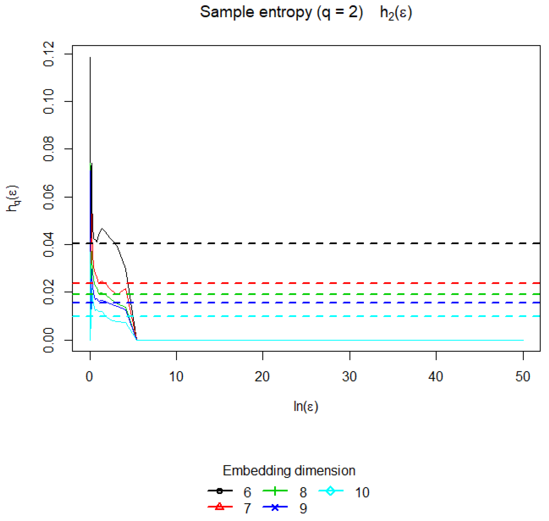
6.3. Sample Entropy

Nonlinear systems characterized by a nonzero sample entropy (also known as Kolgomorov–Sinai Entropy) [30] can possess a mixing property. However, any real system is under the influence of noises of various nature, which, of course, contribute to the mixing in the phase space of such a system. Moreover, from the point of view of strict definition, the Kolmogorov–Sinai entropy when added to the noise system becomes infinite, even if, in the absence of noise, the system exhibits regular motions with zero metric entropy, and the noise intensity is negligible. In such cases, to assess the degree of mixing in the system, they resort to assessing the value of the LLE. Nevertheless, such an estimate cannot always accurately present information on the degree of mixing in the system, since, with an increase in the intensity of noise exposure, the LLE exponent may decrease. In addition, in some cases, the calculation of the Lyapunov characteristics of noisy systems is difficult. The calculation of the sample entropy is also based on the correlation sums (see Figure 8). The value of the sample entropy found in our example is $0.02170441$, which shows a small degree of mixing in the time series.

6.4. Lyapunov Exponents

The LLE characterizing the degree of exponential divergence of close trajectories, a positive value of which means that any two close trajectories quickly diverge over time; therefore, the system is sensitive to the values of the initial conditions, which allows us to identify a dynamic system in terms of the presence of chaotic behavior in it.

Here, we have used the function maxLyapunov for estimating the divergence rates. LLE is found when applying linear regression to them. The value of the LLE which was found in the given example is $0.01382961$, which means that the system (2) is chaotic at $\tau =0.2865$.

Lyapunov exponents were calculated on the whole interval $\tau \in [0.16,0.2865]$ (see Figure 9). Numerical values of LLEs are presented in

Table 1. Nonlinear analysis of time series $V_{1,1}$ of system (2) at $n=0.9$.

	τ	Le_V_11	tau.acf	tau.ami	Emb.dimension	Corr.dimension	Sample Entropy
1	0.220	−0.2116720387	7	4	3	0.3080088	0.001106842
2	0.230	−0.0359923501	7	5	3	1.159866	0.01302575
3	0.240	−0.0035478684	7	5	4	1.048621	0.006855109
4	0.250	−0.0237212132	7	5	4	1.047072	0.008607991
5	0.260	−0.0331964125	7	5	4	1.042478	0.01219783
6	0.270	0.0294146650	7	5	4	1.046891	0.02101408
7	0.280	0.0120013165	7	5	7	1.490351	0.03018144

.

6.5. Bifurcation Plots

The local bifurcation plot (see Figure 1) helps to visualize all types of dynamics generated by the immunosensor model. This graph is plotted as follows: for each value of parameter $\tau$ which is incremented with $0.01$ min steps, immunosensor dynamics were simulated for 1500 generations (150 min). First, 1450 generations were discarded because the immunosensor populations may not have reached the asymptotic behavior. Immunosensor population numbers in the rest of the 50 generations are plotted versus the value of parameter $\tau$.

We see the following qualitative behavior: $\tau <0.22$ corresponds to stable equilibrium; at $\tau =0.22$ bifurcation into a 2-point limit cycle; at $\tau =0.23$ bifurcation into a 4-point limit cycle; then, there is a series of cycle duplication—8 points, 16 points, etc.; at $\tau =0.2865$ chaos (“smear” of points). For $\tau >0.29$, there are some regions where dynamics returns to a limit cycle, e.g., $\tau =0.315$.

With the help of a local bifurcation plot, the system (2) was investigated for different values of $n\in (0,1]$. We can conclude that oscillatory and then chaotic behavior requires the smaller values of $\tau$ at smaller values of n (compare Figure 1 and Figure 10). Moreover, when increasing the values of n, we see asymptotically stable steady states for a wider range of $\tau$ (compare Figure 1 and Figure 11). We can interpret these results from the viewpoint of symmetricity of the diffusion between pixels. We see that symmetric diffusion of antigens between pixels ($n=1$) allows for obtaining stable behavior for the greater values of $\tau$ as compared with unsymmetric diffusion ($n<1$).

7. Discussion

In this work, we consider the model based on lattice differential equations. We note that there are alternatives that are sometimes used for modeling biosensors. For example, in [35], they apply partial differential equations for modeling enzyme biosensor dynamics, which is not applicable for the spatially discrete system of colonies related to pixels. On the other hand, we can consider the model with discrete time (difference equations), which is not suitable with population dynamics of the immune response being continuous within time. As a justification of the lattice model of differential equations for a two-dimensional array of immunopixels, we mention the work [7], where it was used for a wider class of biopixels.

As compared with the previous results, one should bear in mind that here we managed to extend a Lyapunov functional technique for a predator–prey model, which is discretely distributed in space, and it is one of the most important advantages. Such a model is described with the help of lattice differential equations.

Moreover, the stability conditions obtained in the lattice case are similar to a “non-lattice” one. Namely, they are presented with the help of inequalities with respect to time delay. As a result of solving such inequalities, we are able to get lower bound of time delay, enabling us to have global asymptotic stability.

Unfortunately, stability investigation allows us to predict qualitative behavior of the system for some bounded intervals of parameters only (as a rule, for some small values of time delay). More comprehensive research of the system, including chaotic behavior, can be executed with the help of series numerical characteristics, which are traditionally applied for investigation of nonlinear dynamics. As it has already been seen, qualitative behavior of an entire pixels array is determined by particular pixels themselves.

Nonequilibrium properties of the model (2) are determined by the stability of the trajectories of a dynamical system. On the other hand, the main criterion for the chaoticity of the trajectories of model (2) is the positivity of LLE, which provides not only instability, but also many other signs of chaos (non-periodicity, mixing, decaying correlation, positive entropy, etc.). A positive value of LLE (see Table 1), which was obtained for some values of the time $\tau$, is a quantitative measure of the immunosensor model chaoticity.

The study of chaotic processes of model (2) relies on the calculation of correlation characteristics (entropy, dimension, etc.), which make it possible to quantitatively (but still formally) evaluate the interdependence of various sections of a chaotic process and the degree of its self-similarity (fractality, ergodicity).

The embedding dimension is the smallest dimension of the phase space into which the attractor of a dynamic system is embedded (corresponds to the smallest number of independent variables that uniquely determines the steady-state dynamics of the system). When analyzing an embedding dimension calculated for the model (2), we see the growth of a dimension as a result of chaotic behavior (see Table 1).

The separate open problem of the design of a two-dimensional array of immunopixels is related to choosing the value N that determines the number of pixels. One of the solutions of such a problem can use the property of non-extinction of antigens’ colonies. Such an estimate of N can also be obtained as a result of stability conditions.

8. Conclusions

Here, we have considered the model of immunosensors, which is mathematically described by the system of lattice delayed differential equations. The cornerstone of the system is the so-called spatial operator presenting symmetric or unsymmetric diffusion of antigens between pixels.

Using parameter n, the model can be applied in order to simulate both symmetric and unsymmetric diffusion. Comparing Figure 10 and Figure 11, we see that unsymmetric diffusion causes speedup of appearance of chaotic behavior at less values of the delay $\tau$.

When considering the application value of these results in real simulations, we refer the reader to the work [7], where the model based on lattice differential equations of population dynamics was applied for a real sensor of a two-dimensional array of biopixels.

The main results present qualitative research of the model. The global asymptotic stability was investigated. The corresponding conditions are based on the construction of the Lyapunov functionals. They can be presented in the form of inequality including the system parameters and delay. Hence, we get the lower estimation of the delay enabling us global asymptotic stability.

Nonlinear analysis of the model is performed with help of a series of numerical characteristics including autocorrelation function, mutual information, embedding, and correlation dimensions, sample entropy, LLEs. It shows a general tendency of the system from stable equilibrium through Hopf bifurcation to a limit cycle, and then through period doubling to chaos.

We have checked numerical characteristics that were calculated in Section 6 and also with the help of numerical simulation.

The model can be used for any amount of pixels (the number $N\ge 4$). We have seen numerically that its qualitative behavior is characterized by a $4\times 4$ pixels array.