1. Introduction
The missile is the leader in the family of precision-guided weapons. It shows extraordinary combat capability in local wars and has become the protagonist of weapons in modern high-tech warfare [
1,
2,
3]. Due to the high cost, destructiveness and non-repeatability of missile field tests, it is difficult to repeat actual flight tests in large quantities. Therefore, simulation technology plays a key role in simulating the dynamic working condition of the missile in a real tactical environment. Establishing an accurate missile motion model is the premise and foundation of the ballistic simulation experiment. Only the accuracy of the established model is guaranteed, and the simulation results can be of practical significance.
At present, there is much research about missile modeling in the published literature. Among this research, the missile mathematical model established by the mechanism modeling method is commonly used by researchers in simulation experiments. The mathematical model can describe the dynamic and kinematic characteristic of the missile, and clearly show the inherent structure and relationship of the system, reflecting the essence of the process. In [
4,
5], Blakelock et al. systematically expounded the establishment process of the missile mathematical model, and [
6,
7,
8,
9,
10,
11,
12] established the dynamics and kinematics model of missile. There are several problems in this type of research at home and abroad. First of all, it can be found that researchers have to spend a lot of time analyzing the force of the system when using mechanism modeling methods, which makes the research work costly and time-consuming, and it is still difficult to obtain a precise model for describing the characteristics of the whole flight process accurately [
13,
14]. In addition, some assumptions and simplifications are used in the establishment of missile mathematical model. This simplified model has limited description capabilities and low fidelity, which directly affects the credibility of ballistic simulation results. Besides, the inherent mechanism of missile is complex, with non-linearity, strong coupling and time-varying. In the actual flight process, various unintended disturbances are easily suffered by missile. Especially in high maneuvering, large-range and large-profile motion, some mathematical approximations are no longer valid due to some nonlinearities exhibited by the aerodynamic coefficients. Moreover, aerodynamic modeling of missile flight simulation is often based on wind tunnel test data, but a large number of facts show that the flight simulation results based on wind tunnel test data still have large deviations from actual flight data [
15]. It has been clearly indicated that mathematical model including aerodynamic models must be verified using flight test data. in some relevant documents including GJB1395A-2009 [
16] and CCAR-60 [
17]. Furthermore, in the process of digital simulation, only a few feature points are selected to represent the aerodynamic parameters of the whole trajectory. It is one-sided to characterize the whole trajectory dynamic process with these parameters. All of the factors above make it difficult to establish a precise mathematical model close to the realistic plant, so the reliability of the simulation results is poor.
With the advent of big data era, new data analysis methods and innovations have been promoted. The development of intelligent technology provides new ideas for the nonlinear systems modeling. Researchers can obtain massive data from missile flight test. These data can directly or indirectly reflect the state of missile flight process and control effect, and provide a data foundation for data-driven modeling. Therefore, in the big data era, it is of great practical significance to study how to effectively use the flight test data for missile modeling.
The research of nonlinear complex system prediction is mainly focused on various prediction models based on Takens’ theorem [
18]. Various prediction theories and methods of low dimensional chaotic time series are established, such as local prediction method, global prediction method, and nonlinear prediction method based on support vector machine technology, among which global prediction method includes global polynomial predictor, neural network modeling method, etc. Compared with mechanism modeling, data-driven modeling which describes the characteristics of sample data as the criterion, is a ’black box’ modeling technology, directly using the system input and output data to analyze the relationship between system variables. Data-driven modeling is more suitable for nonlinear dynamic system identification and control. In recent years, Neural network and data-driven method are widely used in guidance law and controller design, and it has achieved abundant research results [
19,
20,
21,
22,
23,
24,
25]. There are also some attempts to solve the dynamic system modeling problem by using a hybrid model of mechanism-neural network [
19,
26,
27,
28]. In [
26], Yan et al. proposed a hybrid model structure for aircraft modeling, consisting of basic and additional systems. In [
27,
28], San Martin et al. proposed the use of hybrid models of supervised neural networks for the modeling of dynamic systems.
It can be found that these studies have a common point that they all use the past input and output data of the actual system as input to the identification model. Once the actual system output value is missing, the established identification model will not work. This kind of data-driven modeling method which does not consider the internal mechanism of the system and completely relies on a large amount of experimental data to determine the quantitative relationship between the input and output of the system, is generally applied to the online usage scenarios [
29]. In this scenario, the identification model is treated as an approximator, which is used to control the realistic plant [
30]. In [
31], Hunt et al. provided a survey of nonlinear system neural network modeling applied in the control field. In [
32], Hou et al. made a detailed analysis of the data-driven control (DDC) method, indicating that the input of the neural network approximator includes the input and output of the controlled plant at current moment. In [
28,
33,
34], a data-driven identification model for nonlinear systems is established for optimization of control system and control algorithms design.
Unfortunately, for some special research plants, such as missiles, it is unrealistic to require researchers to measure the realistic output of the missile in real time when simulation experiments are performed on the ground. It must be pointed out that the purpose of establishing a missile model is to replace the actual missile for simulation, not for controlling the actual missile. This offline usage scenarios means that the output of the actual system needed in traditional data-driven modeling will not be available. If the output of the actual system is replaced by the output of the neural network itself and used as an input of neural network, the identification model which is established by the single-step iteration will result in a serious accumulation of errors and the iterative process of identification diverges or converge to wrong values.
At present, few scholars have conducted in-depth research on the modeling of complex nonlinear systems in offline usage scenarios, but its significance in the field of missile modeling is significant. To solve this problem, this paper establishes a missile hybrid model based on flight test data, which can simulate the missile flight characteristics and can be used for simulation and model verification. The unique contributions of this paper are as follows: (i) Aiming at the problems existing in traditional neural network modeling method, a novel hybrid data-driven modeling method is proposed for nonlinear dynamic system modeling in offline usage scenarios. (ii) Based on flight test data, a six-degree-of-freedom(6-dof) missile hybrid model is established, considering the uncertainties and nonlinear factors in missile.
The remaining parts of this paper are arranged as follows.
Section 2 studies the mathematical model of the missile to explain the intrinsic mechanism and dynamic characteristics of the system, and analyzes the specific problems in the mathematical model.
Section 3 analyzes the problems existing in traditional data-driven modeling applied to offline usage scenarios, and proposes a new hybrid data-driven modeling method for offline usage scenarios. A missile hybrid model based on data-driven is designed in
Section 4. Two simulations and some discussions are carried in
Section 5 to verity the feasibility of the proposed method and the credibility of the established model. At last,
Section 6 concludes this paper.
2. Analysis of Problems in Missile Mathematical Model
Modeling is the basis of simulation experiments. At present, the missile mathematical model which is established by researching the relationship between key variables and other measurable variables, is commonly used by researchers in simulation experiments. It includes kinematics and dynamics models. This section studies the internal mechanism and dynamic characteristics of the system through the establishment of missile mathematical model, and analyzes the existing problems.
Mechanism Modeling and Analysis
Before establishing the missile mathematical model, we use several assumptions and simplified conditions as follows [
5,
6]:
The earth is a homogeneous sphere, and the rotation of the earth is neglected;
Missile has an axisymmetric layout form with constant mass and rotational inertia;
This paper studies the case of missile without engine thrust.
Based on the above premise assumptions, a dynamic model describing the missile’s motion in space is established, which mainly includes dynamic equation, kinematic equation, geometric relation equation, height equation and so on [
1,
5,
6,
7,
35,
36].
(1) Dynamic equation of the missile’s centroid motion
is the aerodynamic force of missile received during the flight, expressed in the velocity coordinate system as
m denotes the mass of missile;
denotes the velocity vector of the missile in the ground coordinate system;
is the transformation matrix from body coordinate system to the earth coordinate system;
are the axial force coefficient, the derivative of the normal force coefficient, and derivative of lateral force coefficient, respectively. For aerodynamic axisymmetric missiles,
;
denotes the dynamic pressure;
S is the maximum cross-sectional area of missile;
denotes the angle of attack and
denotes the angle of sideslip.
In summary, the centroid dynamics equation of the missile in the ground coordinate system is expressed as
where
r is the geocentric distance and
is the earth radius. In [
37], Bingwei gave the formula expression of standard atmospheric parameters.
(2) Dynamic equation of missile rotation around centroid
The dynamic equation of missile rotation around the centroid decomposed in body coordinate system can be described as
The component form written on each axis of the missile body coordinate system can be expressed as
where
denotes the rotational inertia,
denotes the component of the rotational angular velocity in the body coordinate system;
are the stabilization moment, damping torque and control moment, respectively;
denotes the stabilization moment coefficient, and
;
are the dimensionless rotation derivatives, and
due to the axisymmetric layout form;
denotes the control moment coefficient;
l denotes the length of the missile.
(3) Kinematics equation of missile centroid motion
To determine the trajectory of the missile’s centroid relative to the ground coordinate system, the kinematics equation of the missile’s centroid motion is established, which is expressed as:
where
denotes the velocity of missile.
(4) Kinematics equation of missile rotation around centroid
To determine the attitude of the missile in space, a kinematic equation describing the attitude change relative to the ground coordinate system is established, which is expressed as
where
denote the pitch angle, yaw angle and roll angle respectively.
(5) Geometric relation equation
The equation is shown in Equation (
8).
where
and
denote the trajectory inclination angle and trajectory deflection angle.
(6) Height equation
The height
h of any point on the ballistic trajectory from the ground is approximated by the following formula:
where
denotes the geocentric distance.
The above equations constitute the motion equations describing the relationship between missile forces, torque and missile motion parameters. It can be seen that the missile mathematical model established by the mechanism modeling method mainly has the following problems. Above all, mechanism modeling is always based on many simplifications and assumptions in the analysis process. The simplified model has limited description capabilities and low fidelity, which directly affects the credibility of ballistic simulation results. Then, the process of establishing a mathematical model through mechanism analysis is cockamamie. It takes a lot of time to analyze the model structure and force, and carry out complex theoretical derivation. Besides, the geometrical parameters of the missile’s shape are not deterministic. There are still slight differences in the aerodynamic configuration and shape even for the same type of missile. Meanwhile, a lot of unknown parameters exist in the mathematical model. For example, in dynamic equation of the missile’s centroid motion (3) and in dynamic equation of missile rotation around centroid (5) cannot be directly measured and are difficult to determine by complex theoretical calculations or expensive wind tunnel experiments. All the factors mentioned above make it difficult to establish a precise mathematical model that approximates the realistic missile, which leads to poor reliability of the simulation results.
3. Hybrid Data-Driven Modeling Method
Traditional neural network modeling typically train offline and used online. This means that the established model and the realistic plant are online at the same time, and the data-driven model is used as a reference model, which is suitable for the optimization of the control system and the design of the control algorithm, so as to realize the control effect of the control system on the realistic plant. Unfortunately, For such a special plant such as missile, it is impractical to repeat a large number of realistic flight tests. The purpose of building a missile model is to replace the realistic plant for simulation experiments. These simulation experiments are carried out without the actual missile, which is called offline usage scenarios. The biggest difference between offline usage scenarios and online usage scenarios is that the output of actual system cannot be measured in offline usage scenarios. Therefore, in view of the problems existing in traditional neural network modeling methods, this paper proposes a novel hybrid data-driven modeling method for complex nonlinear dynamic systems in offline usage scenarios.
3.1. Introduction to Usage Scenario
For most controlled plant, they are nonlinear, strong coupling, time-varying. In addition, there are many uncertain factors such as interference in the actual environment. In the more complex control environment, the traditional control methods cannot adapt to the higher control requirements. To solve this problem, a large number of model-based control methods emerge, such as model reference adaptive control, neural network model predictive control and so on. In these control structures, it is necessary to establish the model of controlled plant, and their usage scenarios are called online usage scenarios.
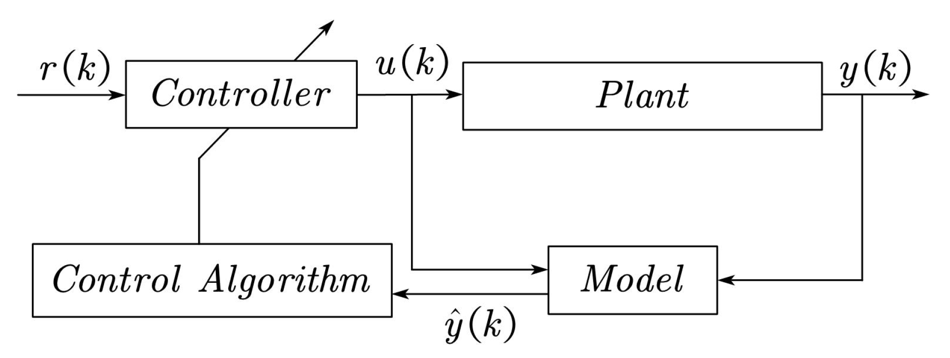
As shown in
Figure 1, the offline trained model and the actual controlled plant are online at the same time, and the neural network model estimates the output of the plant online for the optimization of the control system and the design of the control algorithm.
However, It takes a lot of manpower, material and financial resources to conduct physical experiments. For the control system, the purpose of designing the controller is to control the realistic controlled plant. Therefore, researchers build a model that is similar to the realistic controlled plant by studying and analyzing the process and characteristics of the system, and then use this model to carry out a series of simulation tests. We regard this model usage scenario as an offline usage scenario.
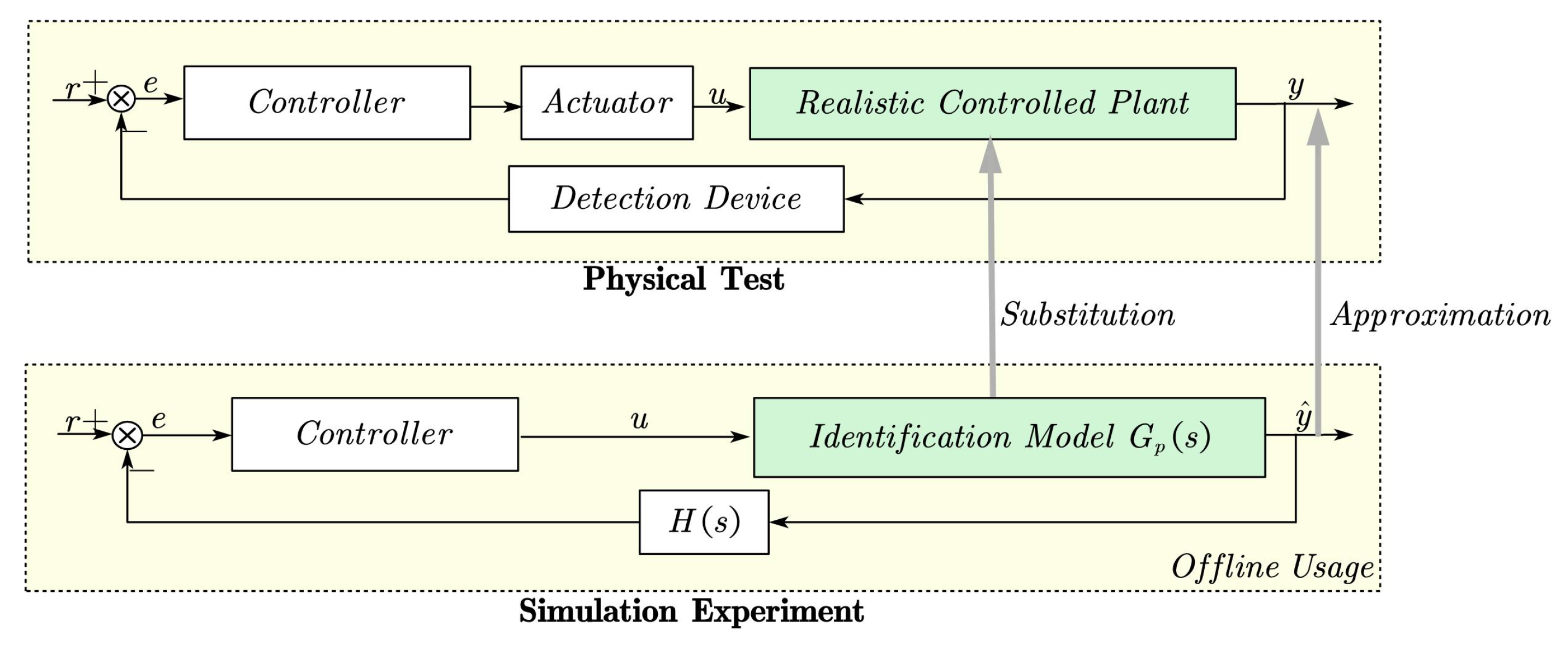
As shown in
Figure 2, there are only controllers and identification models in the offline use scenario, and there is no realistic controlled plant. In this scenario, the purpose of establishing the identification model is to replace the actual research plant for simulation experiment, so as to simulate the control effect of the controller on the actual controlled plant, rather than controlling the actual research plant.
Due to the high cost of some research plants, and many limitations of the experimental site, it is difficult to carry out a large number of physical experiments repeatedly. For such research plants, the established identification model is usually used for offline use scenarios to carry out simulation experiments. Therefore, in this paper, the data-driven modeling method is used to collect test data and establish the ’black box’ or ’gray box’ model of the controlled plant, in order to approximate the output of the realistic controlled plant for simulation experiments.
In addition to the different purposes of modeling, there is a significant difference between the offline usage scenario and online usage scenario, i.e., in the online usage scenario, the actual output of the research plant can be measured in real time, while in the offline usage scenario, there is no actual research plant at all, so this output cannot be obtained. This brings great difficulties to the data-driven modeling of complex nonlinear systems with multiple inputs and multiple outputs.
At present, in the field of single input single output (SISO) nonlinear system modeling in offline usage scenario, researchers regard the model as an approximator and use it to simulate the output of SISO system by transferring new input signals to the offline trained model. However, few researchers have studied the modeling of complex nonlinear systems with multiple inputs and multiple outputs in offline scenarios. Therefore, how to build a data-driven model with high fidelity and put forward a new modeling method to apply to offline usage scenario is worth studying, and is also the focus of this paper.
3.2. Traditional Neural Network Modeling
Common data-driven modeling methods include statistical modeling, artificial neural network modeling, support vector regression and so on. This subsection mainly introduces the traditional neural network modeling method. It is an important nonlinear modeling method and a ’black box’ modeling technique. It uses the past input and output data of the realistic system to construct the expressions of the input variable and the output variable by analyzing the relationship between variables of the system, so that the output
of the model keeps approaching the output
of realistic system. According to the Taken’s theory [
16], most of the nonlinear systems can be expressed as Equation (
11).
where
is the input vector,
is the output vector,
n and
m are the time lag factors of the input and output respectively, and
is a nonlinear function.
According to (11), a neural network approximate model
can be used to replace the unknown nonlinear function
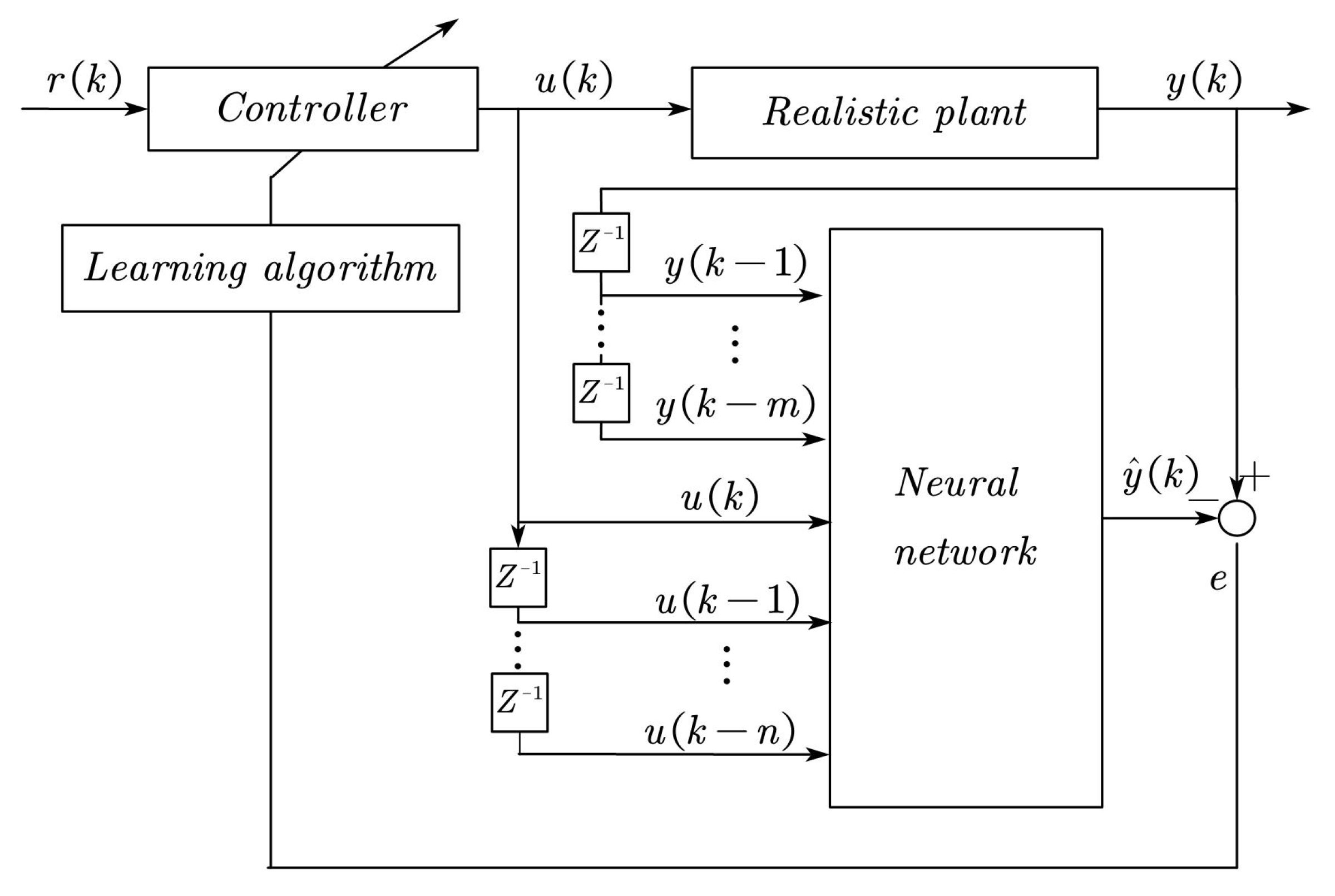
to establish a neural network identification model as shown in
Figure 3, which can be described by (12) for online usage scenarios.
In the online usage scenario, the neural network identification model is used as a reference model, which is online at the same time with the realistic plant, used to control the realistic plant. The input
of the past
n steps of the actual system and the output
of the past
m steps constitute the input vector
(13) of the neural network, and the output
is obtained by the fitting of neural network. Then, the output
of the realistic plant, the output
of neural network model and the error
e between them are sent to the controller. Through the corresponding control algorithm, the control signal
u at the next step is obtained.
It is easy to find that the input
of the neural network in the model established by the traditional neural network modeling method includes the output information of the realistic plant
. For some special plants, such as missiles, the identification model is often used for offline usage scenarios, as shown in
Figure 2. The identification model exists to replace the realistic plant and cannot be online at the same time as the real model, which results a problem that the output information of realistic plant cannot be measured. Once this part of the information is absent, the output
of the actual system in the past
m steps can only be replaced by
, which is obtained by the time delay of the neural network identification model’s output
. It will be used as an input to the neural network along with the input signal
, and the output
will be obtained by neural network fitting, as shown in (14).
It is found through experiments that this single-step iteration makes the output of neural network directly used as its input, which will lead to serious error accumulation, and finally the iterative process diverges or converges to the wrong value, and the output of neural network continually deviates from the output of actual system, so that the identification model cannot be established correctly. Therefore, traditional neural network modeling methods are not suitable for offline usage scenarios.
3.3. A Novel Hybrid Data-Driven Modeling Method
For a nonlinear dynamic system, its input and output are not a static one-to-one mapping relationship. The output of the system at a certain moment is the comprehensive dynamic response of the past input and output. In general, a discrete state space expression for a dynamic system can be expressed as
where
is used to describe the system’s state variables at time
k, which determine the motion of the system.
is the inputs, and its time domain is
. The outputs is
.
and
are the static nonlinear mappings, defined as
,
.
Because there is no realistic plant in the offline usage scenario, the output of the realistic plant cannot be measured, which makes the traditional neural network modeling method difficult to be applied to the complex nonlinear system modeling in offline usage scenario. Moreover, fitting the system’s outputs with neural network directly (14) will lead to serious error accumulation and divergence in the iterative process. Therefore, this paper proposes a hybrid data-driven modeling method to solve the problems.
As shown in
Figure 4, The input of hybrid model consists of two parts, one is the input signal
from the outside at current step, the another part
comes from the interior of the hybrid model at current step.The interior of the hybrid model contains two parts, one is the neural network model built for a key intermediate variables
. If there are multiple key intermediate variables, then multiple neural network models are established in turn. The other part is the mechanism model, which can transform the state variable
into
. One part of the output is transmitted to the external control system, and the other part is transmitted to the internal of hybrid model as the state variables, used as one part of the input of neural network at the same time.
This method avoids using the output of neural network as an input directly. Instead, by analyzing some intermediate variables
that causes nonlinear characteristics in a complex nonlinear dynamic system, which have an input space
and an output space
, fit the intermediate variables based on data-driven approaches. Then, the system’s state variable
is converted into
by the mechanism modeling method so that
, and a hybrid model including neural networks and mechanism is established, which can be expressed as (16).
where
is approximate model of neural network,
is linear mapping function,
is one or more intermediate variables related to the nonlinear characteristic factors of the system, and the next state variable
can be obtained by integrating
.
is one or more system state variables that can cause a change in
.
4. Hybrid Data-Driven Modeling for Missle
In this section, a six-degree-of-freedom (6-dof) missile hybrid model will be established to illustrate in detail how to use the hybrid data-driven modeling method proposed in
Section 3.3.
Missile is a nonlinear multi-input multi-output (MIMO) system with three inputs and twelve outputs according to the mathematical model. To avoid the influence of aerodynamic parameters on the accuracy of the missile model, the acceleration model (3) and the angular acceleration model (5) about the missile’s centroid motion are replaced with neural networks. Then, a hybrid model of the missile containing neural network and mechanism is established based on flight test data. The main steps are as follows:
- Step 1:
Flight test data Preprocessing.
- Step 2:
Establish acceleration model.
- Step 3:
Establish angular acceleration model.
- Step 4:
Establish a missile hybrid model.
4.1. Acceleration and Angular Acceleration Modeling
There are inevitable problems such as outliers, measurement noises, time-domain inconsistency, etc. existing in the measured data. Unprocessed flight test data used directly for hybrid data-driven modeling will reduce the accuracy of the model and even cause the iterative process of identification to diverge or converge to erroneous values. Therefore, the missile flight test data must be pre-processed before using it, mainly including the following parts:
- (i)
Identify, eliminate, and correct the outliers to eliminate signal anomalies, which are caused by external disturbances during flight test;
- (ii)
Data smoothing filtering are used to filter out measurement noise;
- (iii)
Correct the time delay between each measurement data.
It can be known from Equation (
3) that the acceleration of missile’s motion in space is mainly affected by the dynamic pressure
q, the angle of attack
, and the angle of sideslip
. The size of dynamic pressure is determined by the missile velocity
, and
is affected by the position
. The angle of attack and the angle of sideslip cannot be measured directly during the actual flight test, and they are mainly affected by the pitch angle
, the yaw angle
, the trajectory inclination angle
and the trajectory deflection angle
. Therefore, the accelerations
of the three channels are selected as 3 key intermediate variables
in formula (16).
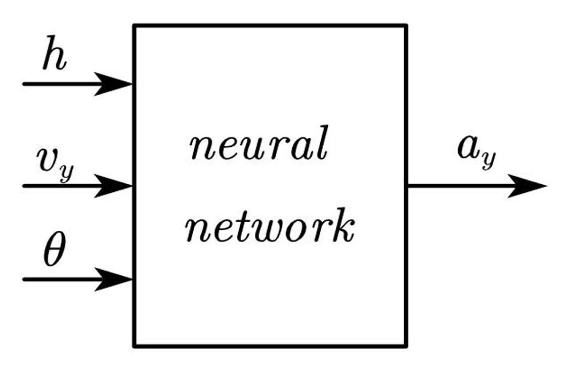
Based on the above analysis, the centroid motion of missile is decomposed into three channels. Taking the pitching channel as an example, the acceleration
of missile longitudinal motion is determined by the current altitude
h, longitudinal velocity
, pitch angle
and trajectory inclination angle
. To avoid the error of pitch angle caused by missile rotation around centroid affecting the accuracy of the acceleration model, the pitch angle is not considered as an input of the acceleration model. Finally, the acceleration model of missile pitching channel is established, as shown in
Figure 5.
The acceleration neural network modeling of rolling and yaw channels is similar to that of pitching channels. The acceleration model of three channels can be expressed as formula (17).
It can be known from Equation (
5) that the angular acceleration of missile in space is mainly related to the current rudder signal
, angular velocity
, dynamic pressure
q, angle of attack
and angle of sideslip
.
q is determined by
and
,
and
are mainly affected by
,
,
, and
. Therefore, the accelerations
of the three channels are selected as 3 key intermediate variables
in formula (16).
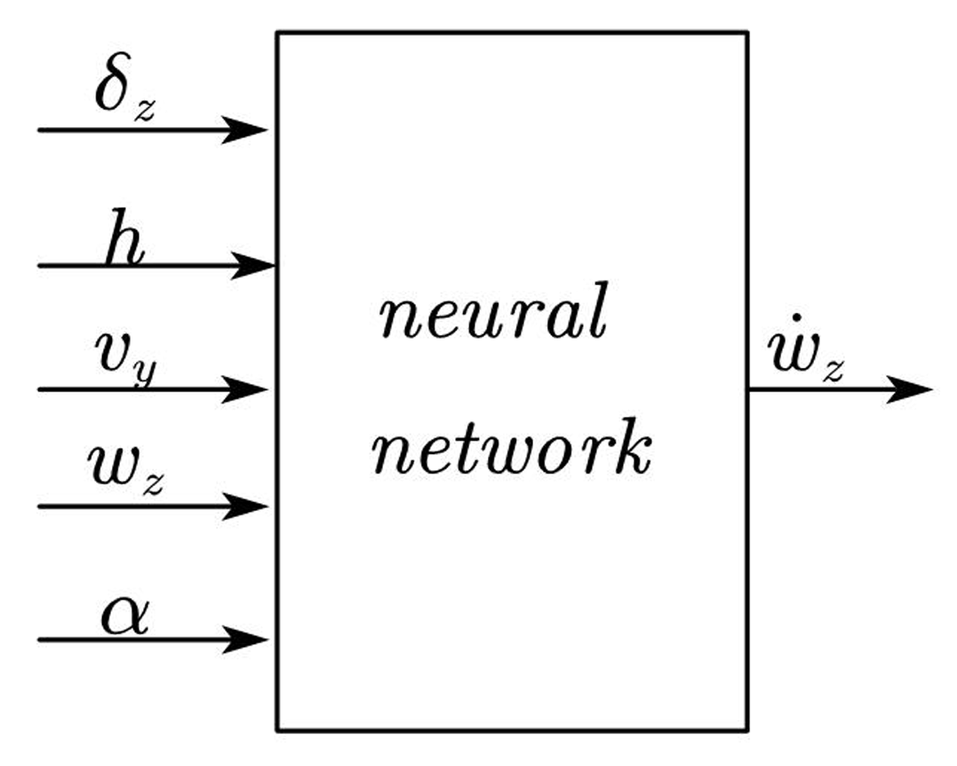
The three-channel decomposition of the missile rotation around centroid is carried out. Taking the pitching channel as an example, the angular acceleration
of the longitudinal motion of the missile is determined by the current rudder signal
, the current altitude
h, longitudinal velocity
, pitching angular velocity
, pitch angle
and trajectory inclination angle
. To simplify the structure of the neural network and improve the fitting accuracy, the measured pitch angle and the trajectory inclination angle are processed by the formula (18) to obtain an angle of attack signal.
Finally, the angular acceleration model of missile pitching channel is established, as shown in
Figure 6.
The angular acceleration neural network modeling of rolling and yaw channels is similar to that of pitching channels. The angular acceleration model of three channels can be expressed as formula (19).
4.2. Establishment of Missile Hybrid Model
Acceleration model and angular acceleration model of pitching, yaw and rolling channels are established in turn. After a series of integral operations and angle calculations, a hybrid model containing the neural network and mechanism model is finally established. The structure is shown in
Figure 7.
The input of missile hybrid model consists of two parts, one is the input signal from the outside, including the current rudder signal , the another part comes from the interior of the model, including the position , velocity , angular velocity , pitch Angle , yaw angle , trajectory inclination angle and trajectory deflection angle at the current moment.
The interior of the hybrid model consists of the acceleration model, the angular acceleration model, three integrators, and angular calculation part. The acceleration model is composed of three neural networks. NN2 represents the acceleration model of pitching channel, and its structure is shown in
Figure 5, where
is obtained from
through NN2. Since the missile has an axisymmetric layout form, the acceleration model of the yaw channel is in one-to-one correspondence with the acceleration model of the pitch channel. NN1 and NN3 respectively represent the acceleration model of rolling and yaw channels, and their structure is similar to NN2 as is shown in formula (17). The acceleration
obtained by the acceleration model is integrated to obtain the velocity signal
, and after another integration, the position signal
is obtained.
The angular acceleration model consists of three neural networks. NN6 is the angular acceleration model of the pitching channel in
Figure 6, which obtains the
according to
,
,
,
and
. Since the missile has an axisymmetric layout form, the angular acceleration model of the yaw channel is in one-to-one correspondence with the angular acceleration model of the pitch channel. As is shown in formula (19), the angular acceleration models NN4 and NN5 of rolling and yaw channels are similar to NN6 of pitching channels, and the output
,
is obtained by fitting the neural networks, respectively.
obtained from the angular acceleration model is integrated to obtain the angular velocity
at next step.
In the angle calculation part, three attitude angles
is calculate from the angular velocity
according to the Kinematics equation of missile rotation around centroid (7). According to the definition of the trajectory inclination angle and the trajectory deflection angle, as is shown in Equation (
9),
and
are calculated.
The output of the hybrid model contains the position, velocity, angular velocity, and attitude angle at the current time. One part of the output is transmitted to the external guidance and control system, and the other part is transmitted to the interior of hybrid model, used as an input to the neural network.
The types and related settings of NN1-NN6 in the missile hybrid model can be the same or different. Several fully connected neural networks can be chosen for the design of hybrid model according to actual needs. For example, BP neural network which is a multi-layer feedforward neural network trained by the error back propagation algorithm is the most widely used neural network, which was proposed by Rumelhart [
38] in 1986. The Radial Basis Function (RBF) neural network has good approximation and global optimal performance, and has high learning and training efficiency [
39]. It has been widely used in modeling, system identification and parameter estimation of complex models. Which type of neural network is chosen to build the acceleration neural network model (NN1-NN3) and the angular acceleration model (NN4-NN6) in the hybrid model is selected by researchers according to the actual training data, training effect and test effect. At present, there is a lack of general theoretical guidance on the determination of neural network structure, which is generally different according to different applications. In practical application, the general adopted method is to constantly try, that is to compare a variety of neural network structures, refer to some constructive opinions, and finally determine a better neural network structure to meet the fitting accuracy.
Through the above steps, a 6-dof missile hybrid model can be obtained. It can approximate the realistic missile, can be used to simulate the flight characteristics of missile, and can be used for simulation and model verification.
5. Simulation Result and Analysis
In this paper, based on flight test data, a missile hybrid model is established by combining mechanism analysis with neural networks.
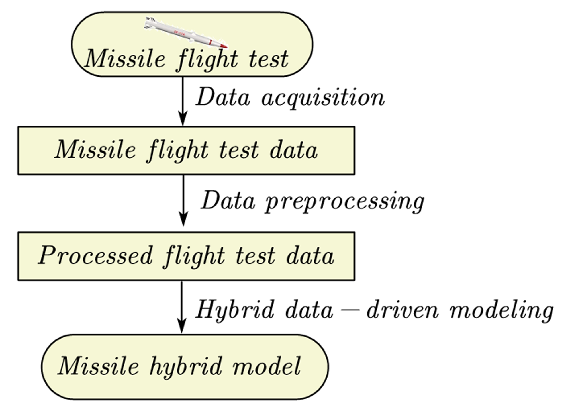
Figure 8 shows the whole process of establishing a missile hybrid model.
In this section, the feasibility of the proposed modeling method and the credibility of the missile hybrid model are evaluated through two simulation experiments and statistical analysis. Firstly, the data collected by the mathematical model is taken as the actual flight test data, used as the training sample set of neural networks. According to the steps in
Section 4, the missile hybrid model is established to verify the feasibility of the method. However, the simulation results obtained by using only one ballistic trajectory data to modeling are contingent, which is not enough to explain the credibility of the established model. A large number of simulation experiments and statistical analysis must be carried out to give corresponding conclusions. Therefore, the Monte Carlo method is used to analog target in
Section 5.2. Data of multiple ballistics under various disturbance factors are collected, and the missile hybrid model is established respectively. Then, the credibility of the hybrid model are verified by statistical analysis of the model accuracy.
5.1. Feasibility Analysis
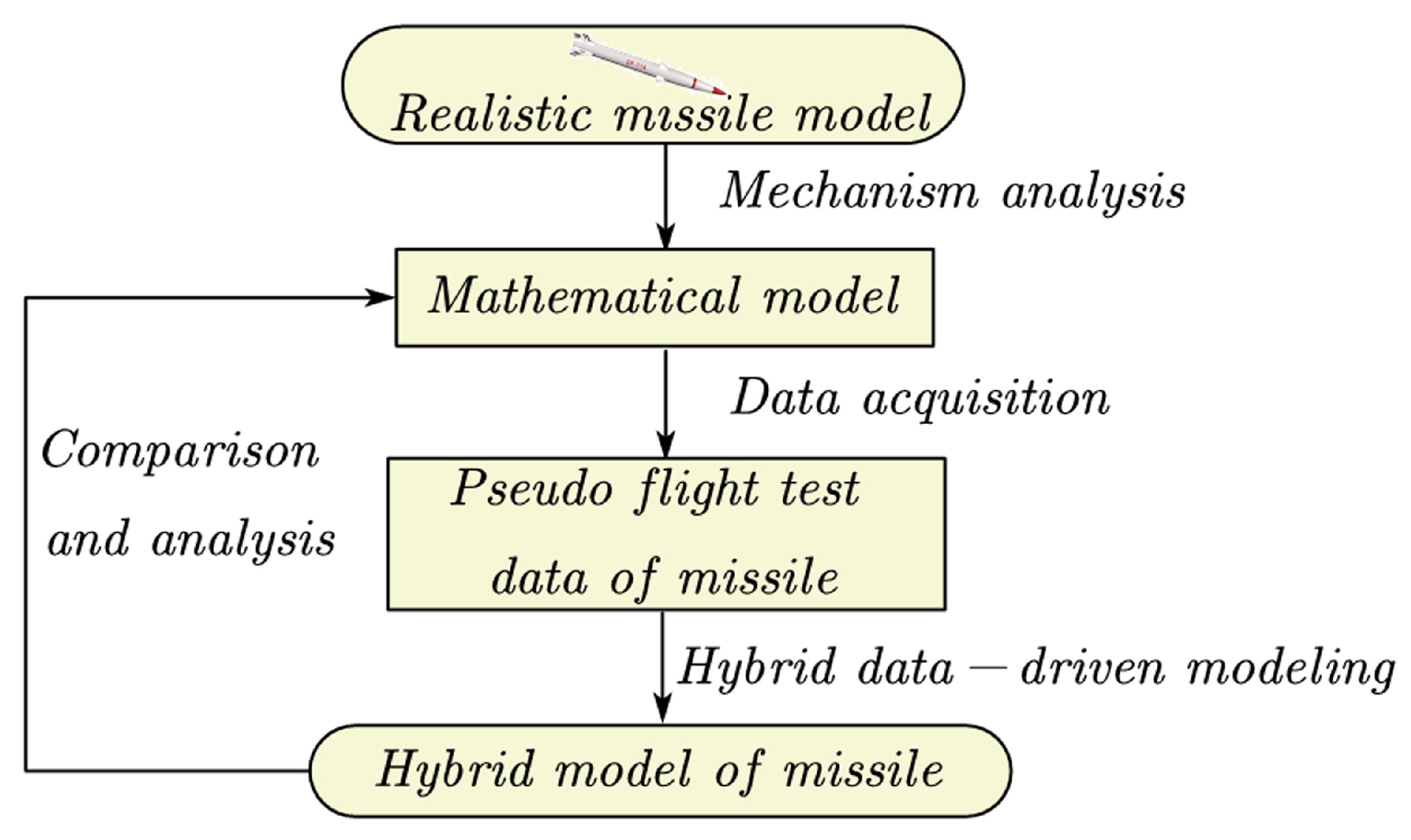
To verify the feasibility of the proposed modeling method, the data collected by missile mathematical model established by the mechanism analysis is used as flight test data, and the missile hybrid model is established by hybrid data-driven modeling method. Finally, the output of the hybrid model is compared and analyzed with the mathematical model. The simulation scheme flow is shown in
Figure 9.
Set the initial launch height of missile to 8000 m, the initial launch velocity is
m/s, the position of target is
m, and the simulation step is 0.005 s. We carry out simulation experiments based on MATLAB/SIMULINK. The solver type we choose is fixed step and the fixed step size (fundamental sample time) is set to 0.005 s. Runge Kutta is a high precision single step algorithm widely used in engineering, so the solver chosen is ode4 (Runge Kutta) [
40,
41]. Neural network toolbox of MATLAB is used to train neural networks. Three acceleration neural network models (NN1–NN3) for rolling, pitching and yaw channels are fitted by 3 BP neural networks. A BP neural network NN1 with 3 layers (input layer, hidden layer and output layer) is used to fit the acceleration of rolling channel. According to Equation (
17), the acceleration of the rolling channel
is affected by
, so NN1 has 2 input nodes and 1 output node. The hidden layer has 6 nodes, and the transfer function is hyperbolic tangent S-type tansig function. The offline Levenberg–Marquardt algorithm is chosen for training. Another BP neural network with four layers is used to fit the acceleration of pitching channel. The acceleration of pitching channel
is affected by three factors
, so NN2 has 3 input nodes and 1 output node. The first hidden layer has 8 nodes, and the transfer function is logsig function; the second hidden layer has 3 nodes, and the transfer function is tansig; the output layer transfer function is linear purelin function, and the training algorithm is the same as NN1. The acceleration of the yaw channel
is affected by
, so NN3 has 3 input nodes and 1 output node. A BP neural network with 3 layers is used to build NN3, hidden layer has 8 nodes, and the transfer function and training algorithm are the same as NN1. After establishing the acceleration neural network models of three channels, 3 RBF neural networks (NN4-NN6) are used to establish the 3 angular acceleration neural network models. The relevant parameters are as follows: Set mean squared error goal to 0.0001, spread of radial basis functions to 1, number of neurons to add between displays to 10. It has been found through the experiment that the ability of neural network to perceive the data with small value and little change is poor, and it is easy to produce iterative error in the modeling process. Therefore, whether to use six neural networks to replace the acceleration model and the angular acceleration model at the same time needs to be determined by the researchers according to the actual flight test data. For example, if the flight test data is collected from a missile with STT(Skid-to-Turn) control mode (
), the angular acceleration model of the rolling channel(
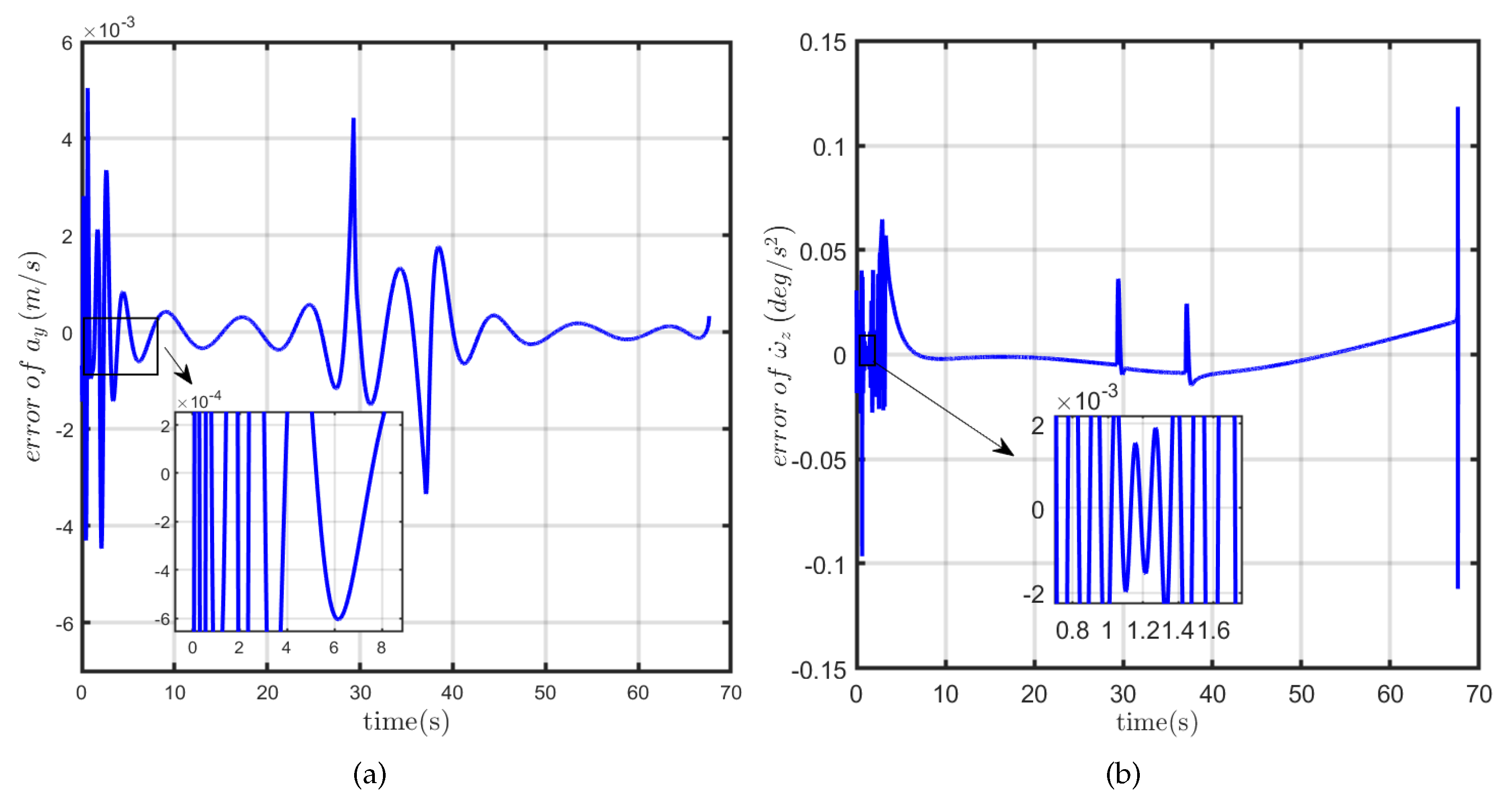
) cannot be replaced by neural network, but mechanism modeling method should still be used to establish the angular acceleration model of the rolling channel. Fitting results and errors of acceleration and angular acceleration model of pitching channel are shown in
Figure 10 and
Figure 11.
From the fitting results of neural network training, it can be seen that the fitting accuracy of acceleration model and angular acceleration model established by BP and RBF neural network both have high fitting precision. The acceleration model and the angular acceleration model of pitching, yaw, and rolling channels are established in turn. Solved by integrating and angle calculation, a missile hybrid model shown in
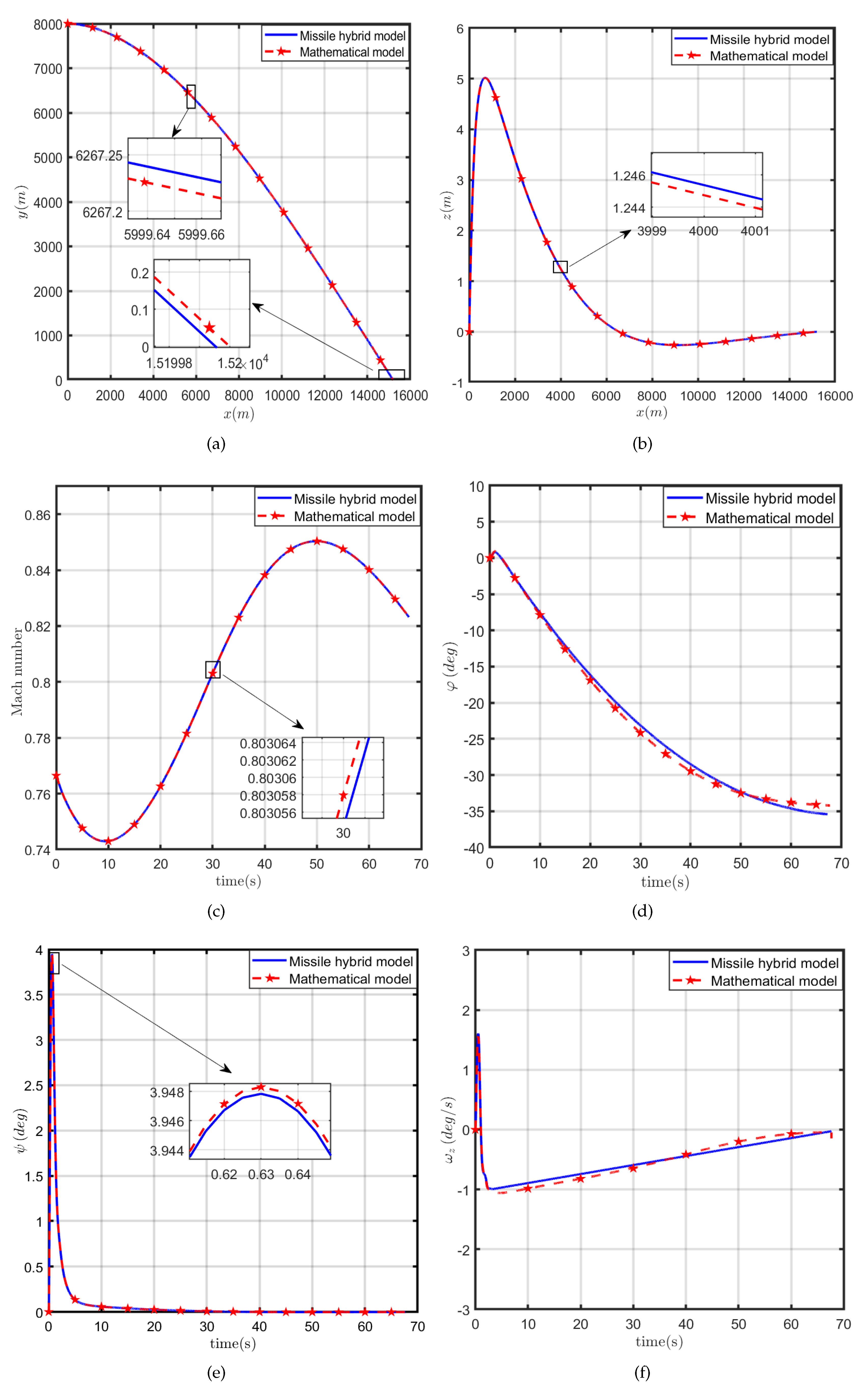
Figure 7 is constructed. The simulation results are shown in
Figure 12.
In this paper, mean square error (MSE) and the mean absolute percent error (MAPE) are used as the evaluation indexes of neural network output.
Table 1 summarizes MSE and MAPE between the 12 outputs of missile hybrid model and the mathematical model, respectively.
From
Figure 12 and
Table 1 it can be seen that the system output response curves of missile hybrid model and mathematical model are substantially coincident, and the errors of each output parameters is small. Instead of directly determine the quantitative relationship between system input and output in traditional neural network modeling method, the hybrid data-driven modeling method proposed in this paper uses the neural network to fit the necessary intermediate variables and combines the mechanism modeling to establish a missile hybrid model. The simulation results show that this method can effectively avoid the serious impact of error accumulation on the model, and the established model achieves high precision, which verifies the feasibility of the proposed method.
5.2. Credibility Analysis
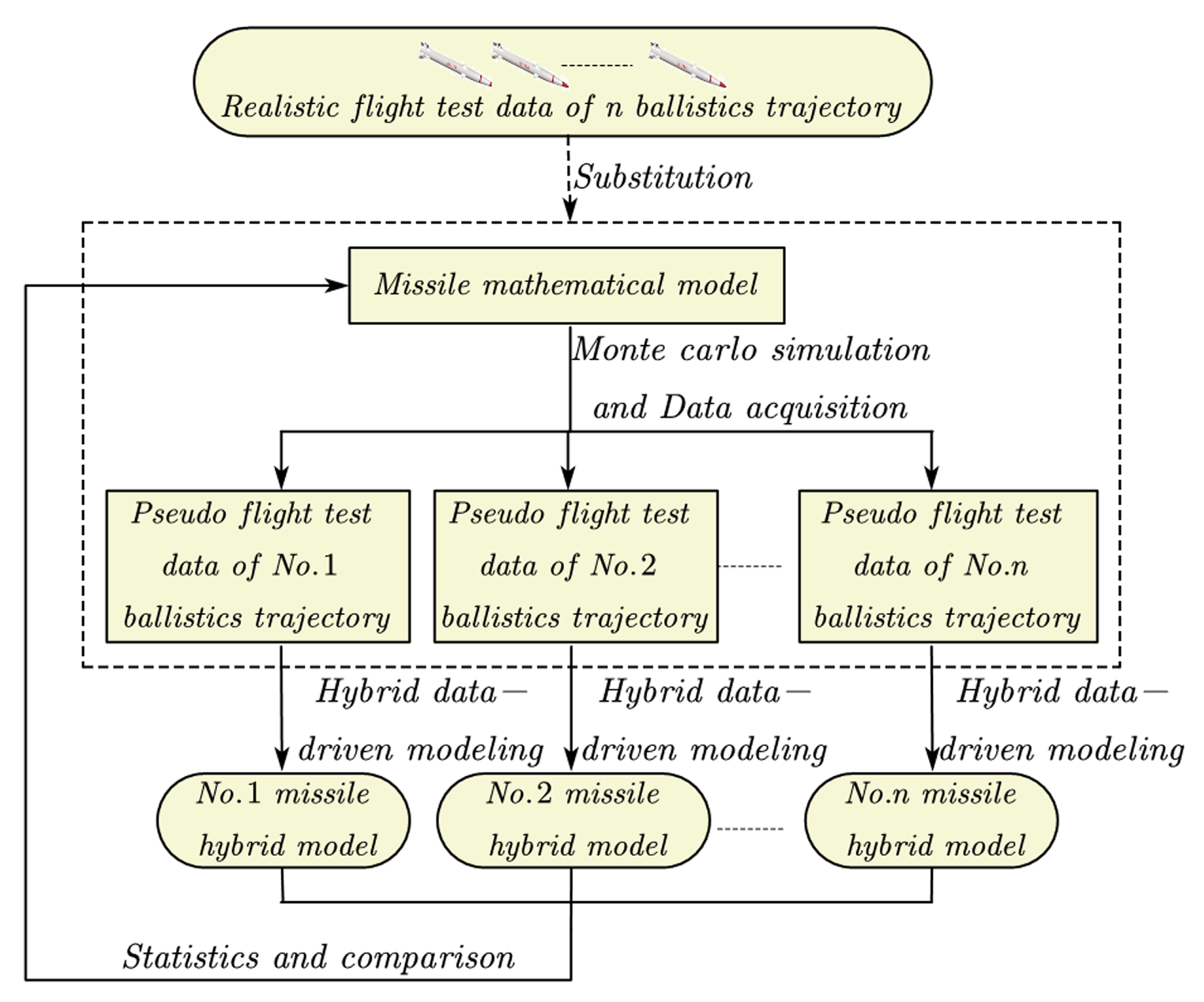
To verify the credibility of the missile hybrid model established by the hybrid data-driven modeling method proposed in this paper, the accuracy of the established model is statistically analyzed based on Monte Carlo method. The simulation scheme flow is shown in
Figure 13.
The basic steps are as follows:
- Step 1:
Establish the mathematical model of the missile by the mechanism modeling method, and the data collected by the mathematical model (pseudo-missile model) is taken as the flight test data of realistic missile.
- Step 2:
Determine the main random disturbance factors encountered during the missile flight and determine its distribution law;
- Step 3:
Simulation target practice of missile is done with Monte Carlo method, and the data of the n collected random trajectories is taken as the flight test data of n ballistic trajectory;
- Step 4:
According to the hybrid data-driven modeling method proposed in this paper, the data of each random ballistic trajectory collected in step 3 is used to establish a missile hybrid model.
- Step 5:
Compare the output results of n missile hybrid models with the pseudo-missile model, and statistical analysis to verify the accuracy and credibility of missile hybrid model.
Remark 1: The Monte Carlo method is a kind of numerical method for solving approximate solutions of mathematical, physical and engineering problems through statistical experiments or stochastic simulations of random variables, also known as statistical experiment or stochastic simulation [
5].
The missile is susceptible to a variety of interference factors during the flight, which makes the missile’s ballistic parameters deviate from the ideal trajectory. Monte Carlo simulation of target shooting (step 3) can quickly use computer simulation instead of flight test. According to the distribution law of various random disturbance factors, the corresponding mathematical probability model is constructed. Then, the random disturbance sampling value is loaded into the 6-dof mathematical model of the missile to simulate the target, and the ballistic state and output parameters of the disturbance trajectory are obtained, which provides the data basis for the experiment in step 4. In this paper, the random interference factors that cause the impact point dispersion are mainly include the following two categories.
- (i)
Internal factors: missile structural parameter errors, mainly including mass deviation, moment of inertia deviation, and aerodynamic coefficient deviation.
- (ii)
External factors: the influence of ballistic wind.
Random errors are added to the parameters, as shown in the equestrian (22):
Where R is a random number, and is the parameter value containing interference.
Table 2 shows the parameter sampling settings for simulation target practice based on Monte Carlo method in step 2.
Table 3 summarizes the statistical values of the drop error and position, Mach number and pitch angle between 10 missile hybrid models and pseudo-missile model, respectively.
According to the statistics, 10 missile hybrid models based on the data of 10 ballistics collected by target practice using Monte Carlo method can successfully destroy the target under the action of control system. The distance when missile and target are encountered is less than 3 meters, achieving a high hit precision. In addition, the hit accuracy of missile is not only related to the accuracy of the established model, but also to the guidance and control law. The mean absolute percent error(MAPE) of is within , the MAPE r of mach number is within , and MAPE of is within . It shows that the missile hybrid model established by the proposed method can fit the position, velocity and attitude well. Taken together, the average relative error of each quantity between the missile hybrid model and the pseudo-missile model is within 7%. It indicates that the hybrid model established by using the data collected from the flight test still has the ability to approach realistic plant and achieve high precision even if the missile is subjected to certain external interference during the flight test in the field.
Compared with the traditional method, the data-driven modeling method proposed in this paper is based on the actual flight test data, using neural network to replace acceleration model and angular acceleration model, considering the interference and uncertainties in the flight process, which can effectively avoid the influence of aerodynamic parameters obtained from wind tunnel test on the accuracy of mechanism model. The hybrid modeling method also avoids using the output of the neural network as its input directly, which makes the identification iteration converges, and effectively establishes the 6-dof missile hybrid model. In addition, the simulation results verify the accuracy of the missile hybrid model under the interference factors, meet the modeling requirements and have high credibility.
