1. Introduction
In the time of Industry 4.0, where the high complexity of manufacturing systems is reflected in multi-criteria optimization problems that must be solved while improving the productivity and sustainability of the production system. Personalized products in Industry 4.0 manufacturing systems are represented by the high-mix low-volume production type [
1]. Adequate evaluation of the cost-time diagram for the high-mix low-volume production type is not capable of describing fully the effects of multi-criteria optimization on a specified production type [
2]. The impact of manufacturing flexibility on this production type is a key optimization parameter, that needs to be well known and described in order to ensure sustainable manufacturing processes [
3]. The research problem concerns the impact of manufacturing flexibility, and the suitability of the multi-criteria optimization methods used on the ability to provide sustainable production [
4]. The impact of the flexibility on the manufacturing systems and their environmental and financial justification is not well described. An appropriately optimized flexible manufacturing system with short flow time and uniformly high machine utilization is a multi-critical optimization problem that can be solved with advanced evolutionary computation methods. When introducing the evolutionary computation method, the complexity factors in the transfer of mathematical methods should be evaluated in the real-world environment. The real-world environment of flexible manufacturing systems that they represent are presented as small and mid-sized enterprises, with specific production characteristics, which advocates a high ability to adapt to the market demand. The high customization level of the customers needs in the manufacturing system, however, results in unevenly occupied, financially unjustified and less sustainable manufacturing systems. Therefore, ensuring highly efficient and sustainable flexible manufacturing systems is very important.
Researchers have recently been paying a lot of attention to ensuring sustainably justified manufacturing systems, defined as [
5]: sustainable manufacturing is the creation of manufactured products through economically-time efficient processes that minimize negative environment impacts while conserving energy and natural resources [
6]. In short: conserve energy (machine and workers’ utilization, short idle times, optimized transport systems etc.), and natural resources (material handling, just in time systems, optimized manufacturing processes and techniques, low material and products scrap). Ensuring sustainable manufacturing systems increase growth and global competitiveness, with sustainable manufacturing optimized processes that minimize negative environmental impacts [
7]. Optimized production methods and operations ensure continuously improving production system performance, cost and time efficiency, product quality, a safer working environment and high flexible manufacturing systems [
8].
Ensuring sustainable production can be ensured through appropriate optimization approaches that optimize multi-criteria optimization problems comprehensively [
9]. However, the evaluation of optimization methods is determined using a cost-time profile diagram [
10]. In the cost-time profile diagram, we are talking about defining the impact of accumulated costs over the time period of orders. Activities, waiting times and resources define the accumulated costs that describe the economically time-efficient production systems, and, thus, minimize negative environmental impacts [
11]. Evaluating the sustainability of manufacturing systems using a cost-time profile diagram identifies single-criteria optimization problems well [
2], but is unable to identify and describe the manufacturing flexibility influence on the manufacturing systems [
12]. The importance of the manufacturing flexibility impact is defined as a four level architecture model within the manufacturing system [
13]. An individual resource level defines the flexibility of the manufacturing system’s resources: labor, machinery and material handling. A shop floor level relates to the flexibility of the production shop floor: routing and operation flexibilities. It is the operation and routing flexibility that defines a flexible job shop scheduling problem as a multi-criteria optimization problem [
14]. In the third and fourth levels of flexibility, we want to define plant and functional level flexibilities, which describe volume, mix, products, modifications, and new product flexibilities. These two levels, thus, represent a typical manufacturing system in Industry 4.0, which defines a high-mix, low-volume production process [
15]. The flexibility defined in this way is a research problem that consists of two parts: multi-criteria optimization of flexible manufacturing systems, and evaluation of the cost-time profile diagram, depending on the manufacturing flexibility [
16]. An appropriately valued and optimized cost-time and manufacturing flexibility ratio ensures a sustainably justified production system that minimizes negative environmental impacts, enhances quality and ensures the company′s global competitive advantage [
13].
The main contributions of the manuscript are: a new method of manufacturing flexibility modelling with a four-level architectural model that describes the high-mix low-volume production type with correlation to an Flexible Job Shop Scheduling Problem (FJSSP). Depending on the production type, we have defined the three machine groups mathematically, according to the parameters of costs, processing times, setup times, energy costs, tool cost, etc. Based on mathematical modelling, a new factor is presented between operational and idle costs. Using a cost-time profile that describes the production characteristics of activity, resources, times and costs, a simulation model is developed using an evolutionary computation method to determine the impact of manufacturing flexibility on the economic and sustainable manufacturing efficiency. The numerical results obtained using the simulation scenario method and two test datasets (Kacem and Brandimarte) that define manufacturing flexibility, represent a new method of a cost-time-flexibility profile diagram, which represents the cost-time investment value as a function of manufacturing flexibility. The encouraging multi-criteria optimization results of the test datasets are supported by an example implementation of the proposed optimization method on a real-world production system. The proposed optimization approach is evaluated by comparing the performance of the self-designed improved heuristic Kalman algorithm (IHKA) evolutionary computation method and the comparative algorithms bare bones multi-objective particle swarm optimization (BBMOPSO) and multi-objective particle swarm optimization (MOPSO), with C-metric measures. The optimization results demonstrate the high ability to use the IHKA optimization algorithm to schedule order optimally in FJSSP production. The proposed algorithm is considered to be the most successful, as confirmed by the numerical and graphical results. Numerical multi-criteria optimization results were transmitted using an interactive method to a simulation environment, where the dependence of the cost-time diagram as a function of manufacturing flexibility is shown. The presented optimization results of a real-world manufacturing system prove the successful transfer of the theoretical mathematical methods through simulation environments to a real-world manufacturing system. The presented research work has shown a high degree of interdependence between the cost-time and the adaptive component of flexibility in the manufacturing systems.
The research work is organized as follows: The second section of the manuscript defines and presents the manufacturing flexibility using a four-level architectural model. The individual levels and their characteristics are defined, together with the impact on the production process. The third section presents a mathematical description of a multi-criteria optimization approach that allows solving complex optimization problems of flexible manufacturing systems with the aim of ensuring sustainable production. The fourth section presents a new approach to defining manufacturing flexibility with respect to the optimization parameters of machine groups, costs, positions and times. The influence is presented of the cost-time profile diagram on the manufacturing flexibility. The results of the manufacturing flexibility modelling are presented in the fifth section, where a new method is described for cost-time investment as a function of manufacturing flexibility evaluation. In the sixth section, the newly proposed theoretical methods are transferred to the applied real-world example, where the input data of a real-world manufacturing system shows the multi-criteria optimization approach with the improved heuristic Kalman algorithm (IHKA) evolutionary computation method. The numerical and graphical results of the proposed method are presented, and the advantages and limitations of the proposed approach are evaluated. Section Seven concludes the paper, with an answer to the initial research question of manufacturing flexibility impact on the provision of sustainable manufacturing systems, identifies the advantages and limitations of the proposed method and approach, and outlines directions and options for further research.
2. Manufacturing Flexibility
Manufacturing flexibility is a multi-dimensional manufacturing objective with no general acquiescence on its definition. This is because every manufacturing enterprise looks on the manufacturing flexibility in its own way. Manufacturing enterprises can define manufacturing flexibility either in an adaptive or proactive manner. The adaptive approach represents the defensive/reactive use of flexibility to accommodate unknown uncertainty in a manufacturing system, and it addresses both the internal, as well as external, uncertainty faced by manufacturing enterprises. An adaptive approach can define manufacturing flexibility as a manufacturer’s ability to adapt or change. On the other hand, a proactive approach to the use of flexibility aids the company in gaining global competitiveness by raising customer anticipation and increasing the insecurity of enterprise rivals. With a proactive approach, we can define manufacturing flexibility as a system’s ability to cope with a wide range of possible dynamical environmental changes. From a sustainable enterprise viewpoint, manufacturing flexibility should be customer-driven, and refers to the availability of personalized products that meet customer needs when there is a demand. From the literature, we can say that it is the ability of a manufacturing system to respond cost effectively and rapidly to changing product needs and requirements [
3].
In this case, the definition reveals clearly that manufacturing flexibility is the ability of a manufacturing system to respond effectively and efficiently to the environmental uncertainties (manufacturing system and global demand). Manufacturing effectiveness related to manufacturing flexibility represents the ability of the system to meet product variety requirements, quantity and at the right time, whereas efficiency represents that all system resources must be planned and scheduled optimally. A general classification of manufacturing flexibility level is presented in
Table 1, where manufacturing flexibility is divided into four levels. In our research work, we are focused on optimizing all four levels of manufacturing flexibility with a new, effective cost-time evaluation method.
The complexity of manufacturing flexibility can be described as environmental uncertainty referring to the occurrence of an unexpected change, both within the manufacturing system and external dynamic changes. Dynamic variability of products within the manufacturing process refers to the flexibility of an advanced personalized variety of products and carrying out different adaptive manufacturing techniques. The dynamic variability of manufactured products can be divided in two different ways. The first way refers to the range of parts produced in the current time high-mix production type. The second way refers to the variation of product output over time, described as the low-volume production type. From the defined high-mix low-volume production type, we can distinguish between two types of changes: planned and unplanned changes. In sustainable manufacturing systems, we want to have as many planned changes as possible, which happen because of some well-planned managing actions. On the other hand, we must eliminate unplanned changes, which occur independently within the manufacturing systems, with unplanned response times. Planned and unplanned changes in manufacturing system flexibility lead to six dimensions: machine, operation, routing, volume, expansion, product and process flexibility. In our research work, we will refer mostly to manufacturing process flexibility, described as: the ability to produce a given set of part types, each possibly using different material, in several different sets of part types that the system can produce without major set-ups [
17], number and variety of products which can be produced without incurring high transition penalties or large changes in performance outcomes [
18].
3. Multi-Criteria Optimization
Multi-objective optimization is an area that deals with multi-objective decision-making of mathematical and combinatorial optimization problems [
19]. Multi-criteria optimization problems involve more than one optimization function, where several variables of the optimization problem need to be optimized. A main characteristic of multi-objective optimization is that there is not only one optimal solution optimizing the optimization function, but, for these functions, there are infinitely many Pareto optimal solutions [
20]. Pareto optimal solutions are non-dominant, Pareto optimal, or Pareto effective. All Pareto optimal solutions in the Pareto space are considered equally appropriate. The field of multi-objective optimization is increasingly present in everyday life, due to the optimization problems′ complexity. Multi-objective optimization can be found in all fields of sciences, economics, logistics, etc., and where it is necessary to make optimal decisions in the presence of trade-offs between two or more conflicting goals [
21].
In a mathematical sense, a multi-objective problem is formulated as presented with Equation (1):
where the integer
k ≥ 2 represents the number of optimization parameters, and
X represents the feasible set of decision vectors. A set of decision vectors is usually represented by constraint functions. A vector-valued objective function is defined as shown in Equation (2):
Minimizing function negative dependence can be made by maximizing the function. The element presents a workable solution or a workable decision. The vector is called the function vector for the feasible solution x*. Limitation of the multi-objective optimization relates to no viable solution that optimizes all of the target functions at the same time. For improving Pareto optimal solutions, at least one compromise of the remaining functions goals must be made.
Using the mathematical notations of Equations (3) and (4), we can conclude that the feasible solution
x1 ∊
X Pareto is dominated by another solution
x2 ∊
X in the case where:
is a feasible solution,
x* ∈
X and the associated output value
f (
x *) is Pareto optimal if there is no other solution that dominates it. The Pareto group of optimal solutions is called the Pareto front. The Pareto front of multi-objective optimization problems is constrained by two vectors:
The nadir vector is defined mathematically by Equation (5):
The ideal vector is defined mathematically by Equation (6):
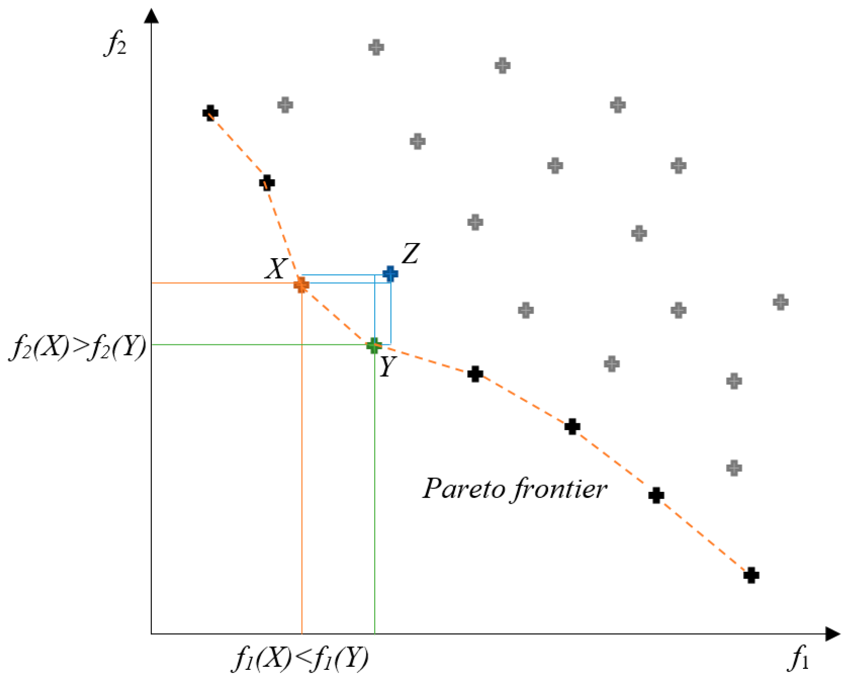
The upper and lower bounds for the optimization functions of Pareto optimal solutions are defined by the ideal and nadir vector components. An example of Pareto optimal solutions is shown in
Figure 1, where there are two optimization functions,
f1 and
f2. The points in the coordinate system represent possible Pareto solutions where the point Z is not defined as the Pareto optimal solution, because it is dominated by the
X and
Y points. The points
X and
Y are not dominated by each other, so we can define both as Pareto optimal solutions.
4. Manufacturing Flexibility Modelling
Modelling of manufacturing flexibility was performed on the flexible job shop scheduling type of manufacturing system. The multi-criteria nature of the flexible job shop scheduling manufacturing type is described as: we have n jobs which can be performed on m machines from a set of machines (j = 1, …, m) suitable for carrying out the jobs. The choice of using which machine is made according to the machine occupancy and the suitability of the individual machines to perform the operation. The number of jobs n and number of machines m are given. Each job i has a specific sequence and number of operations Oi. The processing time of the operation pjk may vary, depending on the machine on which it is performed. For the multi-objective flexible job shop scheduling problem, some limitations must be made:
One machine can process only one job at a time.
One job can be processed only on one machine at a time.
When the operation starts it cannot be interrupted until the end of the operation; after completion, the next operation can start.
All the jobs and operations have equal priorities at the time zero.
Each machine m is ready at time zero.
Given an operation Oij and the selected machine m, the processing time pij is fixed.
The multi-criteria flexible job shop scheduling optimization problem involves optimizing three criteria, described by Equations (7)–(9).
Makespan (time required to complete all jobs):
Maximum workload (workload of the most loaded machine):
Total workload of all machines:
where
Cj is the completion time of job
Ji, and
xijk is a decision variable on which individual machine the operation will be processed.
Considering the definition of manufacturing flexibility in
Table 1, we can see that a flexible job shop scheduling problem is defined as manufacturing flexibility according to the shop floor level (routing and operation flexibility associated with a shop floor). For more detailed modelling of manufacturing flexibility, we must still define manufacturing flexibility with respect to the other three levels: individual resource level (labor machine and material handling flexibility associated with a resource), plant level (volume, mix, expansion and product flexibility associated with a plant) and functional level (manufacturing flexibility). For addressing manufacturing flexibility comprehensively, we present below multi-criteria optimization modelling and the impact of manufacturing flexibility on sustainable production systems in relation to the cost-time-flexibility dependency. The benchmark data sets were expanded with additional data of the production system related to costs, manufacturing flexibility, dimensions and setup times. Additional data were generated mathematically, except for the location of the machines, which was a constant. In order to ensure adequate data interdependence and the veracity of the results, we decided to divide the machines into the three groups, as shown in
Table 2. With the help of additional data from the real-world production system, we upgraded the simulation model. Such a model offers a comprehensive analysis, comparison, upgrade and evaluation of real-world manufacturing systems.
Table 2 shows three machines groups, divided by the operating costs of the machine EUR/h. The three groups of machines are divided into small (
G1), medium (
G2) and large machines (
G3). The price range of operating hours is between 30 to 40 EUR/h for small machines, 40 to 50 EUR/h for medium and 50 to 60 EUR/h for large machines. We assumed real values of fixed costs and recalculated the idle cost of the machines using the literature [
22]. A detailed recalculation of machine prices is shown below. The recommendations given in the literature [
22] have defined fixed costs as 40% in the case of a small machine, 50% in the case of a medium-sized machine, and 60% of a fixed cost in the case of a large machine. The right column of
Table 2 shows the factor between fixed and recalculated idle cost values used by the computer program as a constant value in a mathematical calculation assignment.
The specified limits for the individual variables interval were generated by the numerically generated data, independently for each machine, and the data are shown in
Table 3. The data are correlated with their correlation factors. The correlation of the generated data ensures the credibility of the simulation and numerical results. The data of the production system can be varied according to changes, and the mathematical and simulation model will adapt it automatically. The presented approach allows modularity and high flexibility of the entire proposed solution for simulating multi-objective optimization problems. The key advantage is the modular composition and easy adaptation to different types of manufacturing or service enterprises.
Table 3 shows additional numerically generated data from the production system, which, in addition to operational and idle costs, shows the locations of the machines with respect to the base coordinate system with (two)
x and
y axes. The last row of the Table lists the setup time, which plays a key role in evaluating production flexibility against a cost-time diagram.
Table 4 shows the determination of the variable costs of the machines according to the three machine groups. The calculation of variable costs was carried out using the calculation given in the literature [
22]. The basic initial properties were assigned to the calculation:
The production system operates in two shifts,
Financing the purchase of machinery, 50% own funds, 50% loan with 8% interest,
Electricity value constant 0.2 EUR/kWh,
4% maintenance cost,
Facility costs EUR 100/m2 and
4% additional operating costs.
The Impact of Cost-Time Profile on Manufacturing Flexibility
The main advantage of a flexible production system is its adaptability to customers demands. Simulation modelling of a flexible job shop scheduling problem is an almost unexplored area, so we wanted to prove the link between cost, time and production flexibility on all four levels of manufacturing flexibility by introducing functional dependency. The use of advanced optimization algorithms and simulation models improves and balances the interdependence between these three parameters significantly. As a basis for investigating the impact of production adaptability, we have chosen the well-known cost-time profile (CTP) method [
10]. The CTP diagram is based on value stream architecture (VSA) [
23], and for the purpose of visualizing the production process, shows the connection between the three main components (resources, activities and waiting times). Traditional cost accumulation deals only with the aspect of production, while VSA emphasizes operating procedures and the use of different resources, notably time, but does not take costs into account. In response to this shortcoming, which takes into account both cost and time considerations, researchers have proposed the introduction of the CTP method [
2]. CTP is a graphical representation of the production orders costs sum in a given time unit. This model represents the source information from the moment the production process begins to the moment the order with the completed activities leaves the production process. The basic components of CTP are defined as:
Activities: There are two assumptions about activities. The first is that the cost of the activity is incurred continuously from start to finish of the activity. The second is that the resources must be ready for use before the activity begins. In CTP, activities are represented by a linear function dependence with a positive directional coefficient.
Resources: In CTP, sources are staged with vertical lines, as they are always available at the time we need them. In addition, their costs are added to the total cost of the contract immediately. When the cost of resources is added to the cost of the product, it is treated as part of the cost that has been spent, and will not be reimbursed until the completion of the order (product sale).
Waiting: It is defined as the sum of moments during which no activity occurs. It is assumed that, while waiting for the implementation of the activity, its costs do not increase. The fact that waiting costs do not increase in this activity is presented in the CTP as a horizontal line. Activity waiting periods are very important, because it is widely known that there is a considerable amount of time during which there is no added value to production processes. This time does not affect the cost of the order directly, but extends the time before the order is shipped.
Total cost: Total cost represents the addition of all direct costs incurred in the production of the contract, without already being taken into account in the CTP diagram. The total cost is reflected in the amount at the time the order is completed.
Cost-value investment: It is represented by a surface area below the CTP line, which represents how and how long the costs have accumulated during the production process. The surface area under the CTP represents the cost-time dimension.
Direct costs: Represent the total amount of total costs and investment costs.
Figure 2 shows an example of a time-value diagram with the components defined above. The orange colored components represent the resources, the green colored arrows represent the activity, and the blue colored arrows represent waiting.
We have expanded the two-dimensional cost-time function dependency with an additional feature that describes the manufacturing flexibility. We have identified the missing required data shown in the Tables below.
Table 5 shows the mathematically assigned material cost values for individual orders. We labelled the values of the material costs that were allocated mathematically in the interval between 20 and 30 EUR per order
Pm. Material costs’ values had to be assigned in order to provide a credible CTP. The material needed to execute the order is identified as the source of the CTP diagram.
Table 6 and
Table 7 define the number of products per order. The number of order products ranges from the value of one product in the reference scenario
Rs, to 20 pieces of the product per single order in the scenario
S2. The introduction of the simulation scenario method represents the possibility of testing and responding the simulation model to different changes in the production system. In our case, the three simulation scenarios define manufacturing flexibility as, fully customizable production in the R
S scenario, where each order represents one piece of product. By increasing the number of products within the order in scenario
S1 (1 to 10 pieces) and
S2 (10 to 20 pieces), here, the production is defined as less flexible. The number of product pieces in
Table 5,
Table 6 and
Table 7 is represented by label
Pq. The
Pq values are assigned numerically according to the distribution function and the interdependence of the production parameters. The simulation scenarios designed in this way allow us to analyze the impact of manufacturing flexibility on the cost-time profile diagram.
5. Manufacturing Flexibility Modelling Results
Table 8 shows the simulation results of modelling the impact of the manufacturing flexibility on the CTP diagram. Simulation and mathematical modelling are performed using simulation scenarios with the aim of changing the manufacturing flexibility parameters. Simulation experiments were performed on five benchmark datasets (Kacem 5 × 10, Kacem 10 × 10, Kacem 15 × 10, Mk08, Mk10) [
24,
25]. Performing simulation experimentation on two different datasets allows the verifiability and credibility of the obtained optimization results.
The results presented in
Table 8 are crucial in evaluating the CTP diagram and the impact of manufacturing flexibility on it. The average machine utilization decreases as production flexibility increases. The above mentioned flow time in
Table 8 certainly affected the machines’ utilization and, consequently, the average throughput of the product [pcs/h], which increases with increasing manufacturing flexibility. The biggest impact is flexibility when it comes to costs that go down when we produce several identical pieces in the manufacturing process.
As a result of the proposed simulation modelling approach, with the introduction of all additional characteristics of the production system,
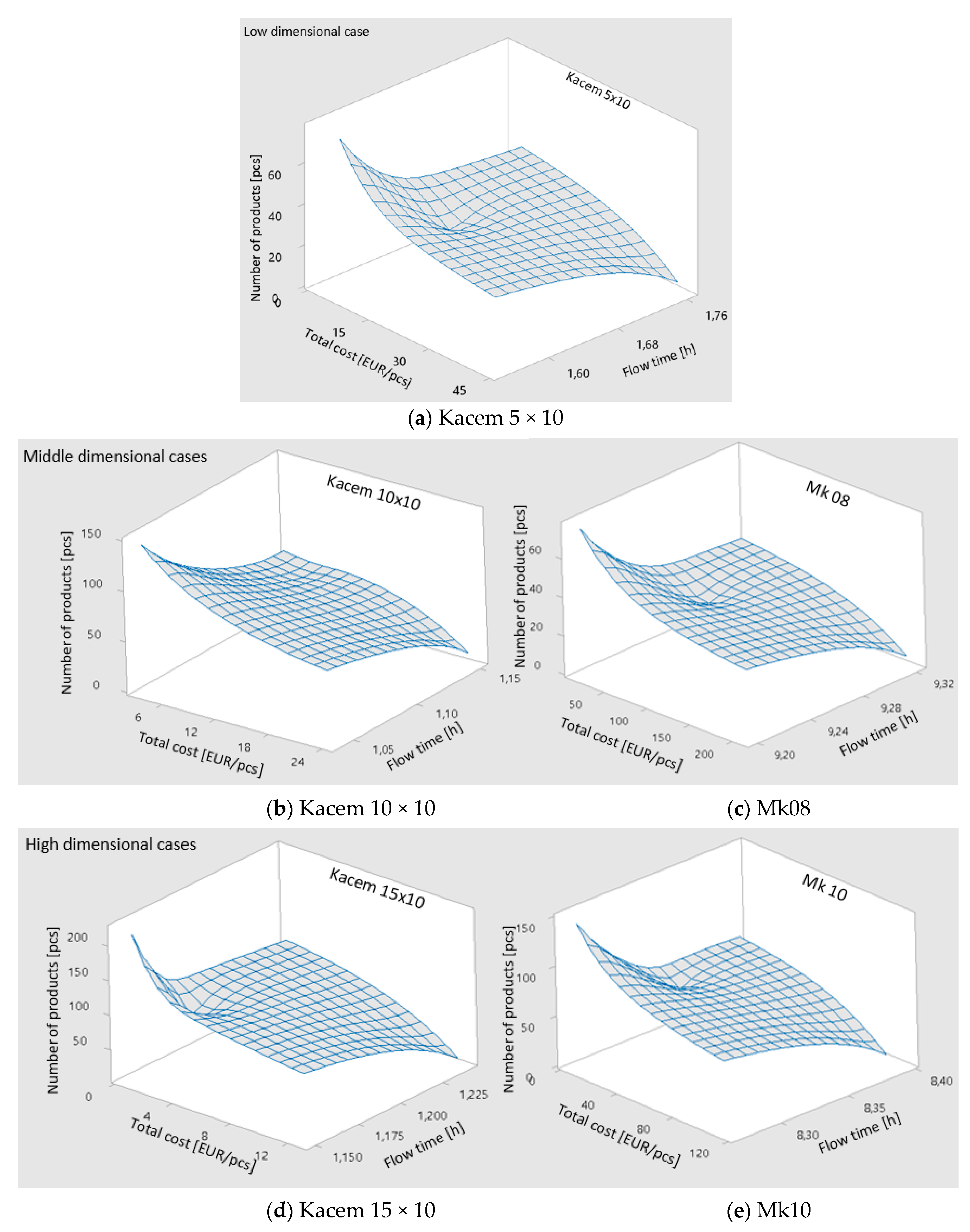
Figure 3 shows the final results after simulation and numerical studies of the manufacturing flexibility impact on the CTP diagram.
Cost-Time-Flexibility Profile Diagram
The cost-time profile diagram, depending on manufacturing flexibility, is modelled graphically using the numerical and simulated results shown in
Table 8. We named the three-dimensional diagram a cost-time-flexibility profile (CTFP). As with the analysis of the IHKA optimization algorithm, its suitability was tested on low, medium and high dimensions. It was noted that the shape of the three-dimensional diagram is influenced by resources, activities and waiting times, depending on the flexibility of the manufacturing process, as shown in
Table 8. The basic cost-time diagram uses linear dependencies and constant values. With the CTFP graphical results in
Figure 3, we can see nonlinear dependencies of the three variables (cost, time and manufacturing flexibility). Unlike the surface that describes the cost-time investment in a two-dimensional graph, the three-dimensional graph is a volume that describes the cost-time investment depending on the manufacturing flexibility.
For all five datasets, divided into three groups regarding dimensional difficulties, we see the adequacy of solving the optimization problem and the corresponding dependence between the variables in the CTFP diagram. We define the differences between the results of individual CTFP diagrams as:
The Kacem 5 × 10 low dimensional case shows a rapid increase in costs as production flexibility decreases. An additional feature of the graph is the average cost and flow times in the first third of the diagram, which is attributed to the small number of orders.
The Kacem 10 × 10 medium dimensional case shows a continuous dependence of three variables, with no additional features detected within the three dimensional diagram. The interdependence in this case shows a linear dependence, the volume of the area below CTFP represents a steady dependence between time-cost and manufacturing flexibility.
The Mk08 dataset shows a high dependence on cost, processing time and flexibility, which is represented by the slope of the diagram in the upper third of the diagram when flexibility is at its highest. An additional feature is the strong correlation between higher costs and flow time in the mean values. In this case, the production flexibility variable is also located in the middle value range.
High-dimensional optimization problems (Kacem 15 × 10 and Mk10) show a significant dependence on the three parameters mentioned above to ensure production viability. Cost reduction and shorter processing times are influenced significantly by the flexibility of production, especially when increasing the number of orders.
In general, we find that the CTFP diagram is influenced significantly by the flexibility of production, and its dependence on increasing orders is demonstrated by the CTFP diagram. The CTFP thus proposed illustrates graphically and numerically the situation within the production system. From the presented optimization, the approach of multi-criteria optimization and manufacturing flexibility modelling, it can be summarized that: Higher and even machines’ utilization allows energy consumption reduction at the time when the machines are waiting for the operation to be performed (shorter idle time). Shorter flow times without intermediate waiting times allow quick adaptation to demand, and a high level of customer satisfaction on short delivery times (shorter due dates). Properly scheduled orders, depending on the execution of individual operations, allow shorter and more efficient transport routes and effective just in time method use. Proper allocation of operations to highly efficient machines with shorter processing time and high efficiency ensures low waste and efficient use of materials and energy resources. Effective work assignments with regard to the cost of operation and waiting defined by the flexibility of production and the division of machines into three groups make the production system highly economically viable.
6. Manufacturing Flexibility Case Study
With the proposed comprehensive approach and associated methods in the previous sections, we proved the high ability to solve multi-criteria optimization problems of flexible manufacturing systems, so we decided to test the whole approach in the case of multi-criteria optimization of a real-world manufacturing system.
The ability to solve a multi-criteria optimization problem of a real-world manufacturing system (data set labelled as RW_PS) is presented in
Section 6. The first part of the section presents the real-world input data of the manufacturing system, which enables multi-criteria optimization of flexible job shop production. In the real-world case, only relevant and credible input provides the ability to achieve reliable optimization results. The following is an example of solving the scheduling of fifteen orders and comparing the results of the IHKA algorithm with the optimization solutions of the bare bones multi-objective particle swarm optimization (BBMOPSO) and multi-objective particle swarm optimization (MOPSO) algorithms. The transfer of optimization results to the simulation environment is presented following the previously proposed method of evaluating the sequence of machine operations determined by the IHKA algorithm. A modular and flexible simulation model has been built to provide an automated and easy interface to handle the simulation model [
26]. The following is the analysis and evaluation of the simulation model using the CTFP diagram, which is proposed as part of a comprehensive multi-criteria optimization approach of the manufacturing system.
6.1. Manufacturing System Input Data
The selected data were obtained from a European medium-sized company that manufactures custom products (high-mix, low-volume production type). Orders received in the company, ordered by the subscribers, must be scheduled optimally on the available machines within the production system. The orders input data are presented in
Table 9. The orders consist of three different product types with different processing times, machine usage cost, machine idle rates, setup times and number of operations. The information provided by the company and the updated recalculated usage and idle cost values of the machines is formulated mathematically, as presented in the previous section. According to the literature [
22], real-world production type is defined as flexible job shop production type. Compared to the Kacem and Brandimarte [
24,
25] test datasets, we have found that different product types add additional complexity of the RW_PS optimization problem. A parallel can be drawn between the Brandimarte datasets and the inputs of the real-world production system (RW_PS), both of which data sets allow operations to be performed on only a few specific machines within the production system.
For real production system data, machines marked M1 to M12 represent the following operations:
M1 and M2 cutting of raw material,
M3 to M6 manual welding,
M7 and M8 robotic welding,
M9 is a color coating operation,
The assembly operation is performed on two available machines M10 and M11,
The M12 is a final control operation.
The main task of the optimization algorithm is to determine the order of operations on the available machine optimally. In doing so, the algorithm must determine which of the machines will execute which order, while optimizing three key parameters: makespan, maximum machine utilization and eliminating any bottlenecks in the manufacturing system.
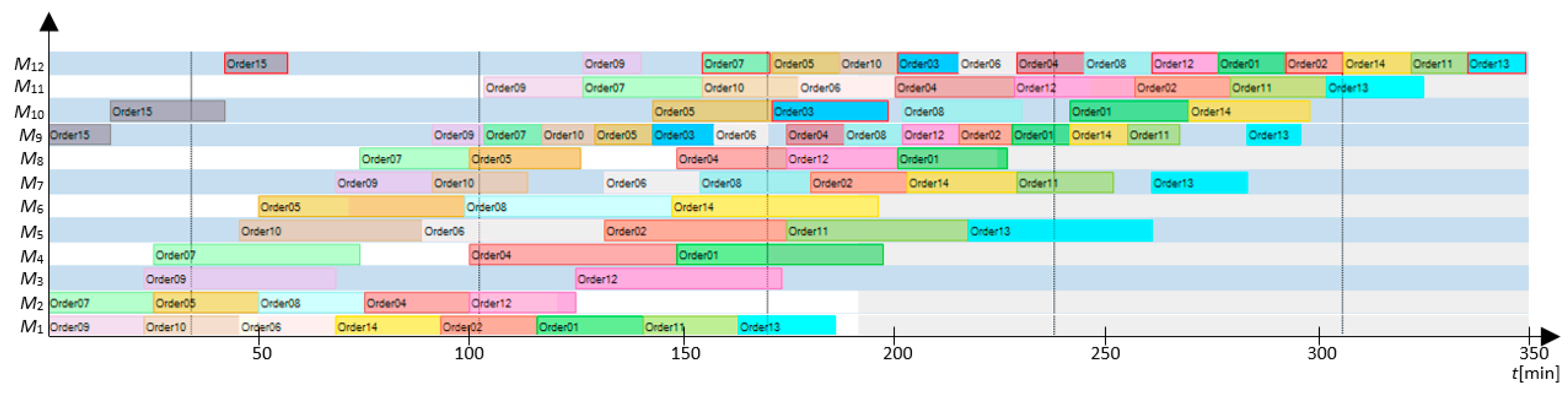
6.2. IHKA Multi-Criteria Optimisation
The production system input data shown in
Table 9 and the order input data, performs multi-criteria optimization of custom production scheduling using the IHKA algorithm [
26]. In
Figure 4, the Gantt chart provides a solution for scheduling orders and individual operations according to the machines available. The IHKA optimization algorithm performed the optimization with three key parameters: makespan, total machine utilization and utilization of the most busy (bottleneck elimination). The Gantt chart in
Figure 4 shows that all orders are executed within 348 min. In order to determine the performance of the IHKA algorithm in solving real-world optimization problems, an analysis and comparison of optimization results was performed, with the currently most up-to-date algorithms for solving the flexible manufacturing scheduling of MOPSO and BBMOPSO.
A performance measures analysis was performed of the proposed IHKA optimization algorithm and the comparative algorithms BBMOPSO and MOSPO. Due to the complexity of the optimization problem, the comparison of the algorithms’ performance was performed using the C-metric method [
27]. Numerical results of thirty interactions calculation for the C-metric performance measures method and the labels meaning are presented in
Table 10:
Min value represents the worst Pareto front position obtained from the state of the subject algorithm which dominates the object algorithm in a certain number of percentages.
Max value represents the best Pareto front obtained by the subject algorithm, which dominates the object algorithm in a certain number of percentages.
Mean value represents the performance of the algorithm in the subject column, and its dominance over the algorithm in the object column. The higher the value, the higher the performance of the algorithm in the subject column is.
Std value represents the performance of the algorithm in the subject column and its stability relative to the algorithm in the object column. The lower the value, the higher the stability of the algorithm in the subject column is.
Table 10 shows the numerical results of the C-metric performance measures analysis within thirty interactions, comparing the obtained results of the individual algorithms:
The IHKA algorithm with 95.9% dominates the BBMOPSO algorithm with associated high stability of 6.17%. High performance of the IHKA algorithm is also proved in comparison with the MOPSO algorithm, which IHKA dominates with 85.94%, with stability percentage of 43.33%.
The BBMOPSO algorithm dominates the IHKA algorithm only with 6.03%, which shows a low degree of dominance, with a corresponding 13.24% stability percent. The BBMOPSO and MOPSO comparative algorithms dominate each other, with 10.28%, and a stability percentage of 20.02%.
The MOPSO algorithm has a low degree of dominance compared to the proposed IHKA algorithm, and the stability percentage is also high, which shows low stability. Cross-referencing the comparison algorithms shows the dominance of the MOPSO algorithm, with 75.64% versus BBMOPSO and a stability percentage of 29.47%.
Numerical results shows high performance with respect to the dominance and stability criteria of the proposed IHKA optimization algorithm compared to the comparative algorithms. The proposed algorithm demonstrates a high degree of capability and robustness of solving multi-criteria optimization problems.
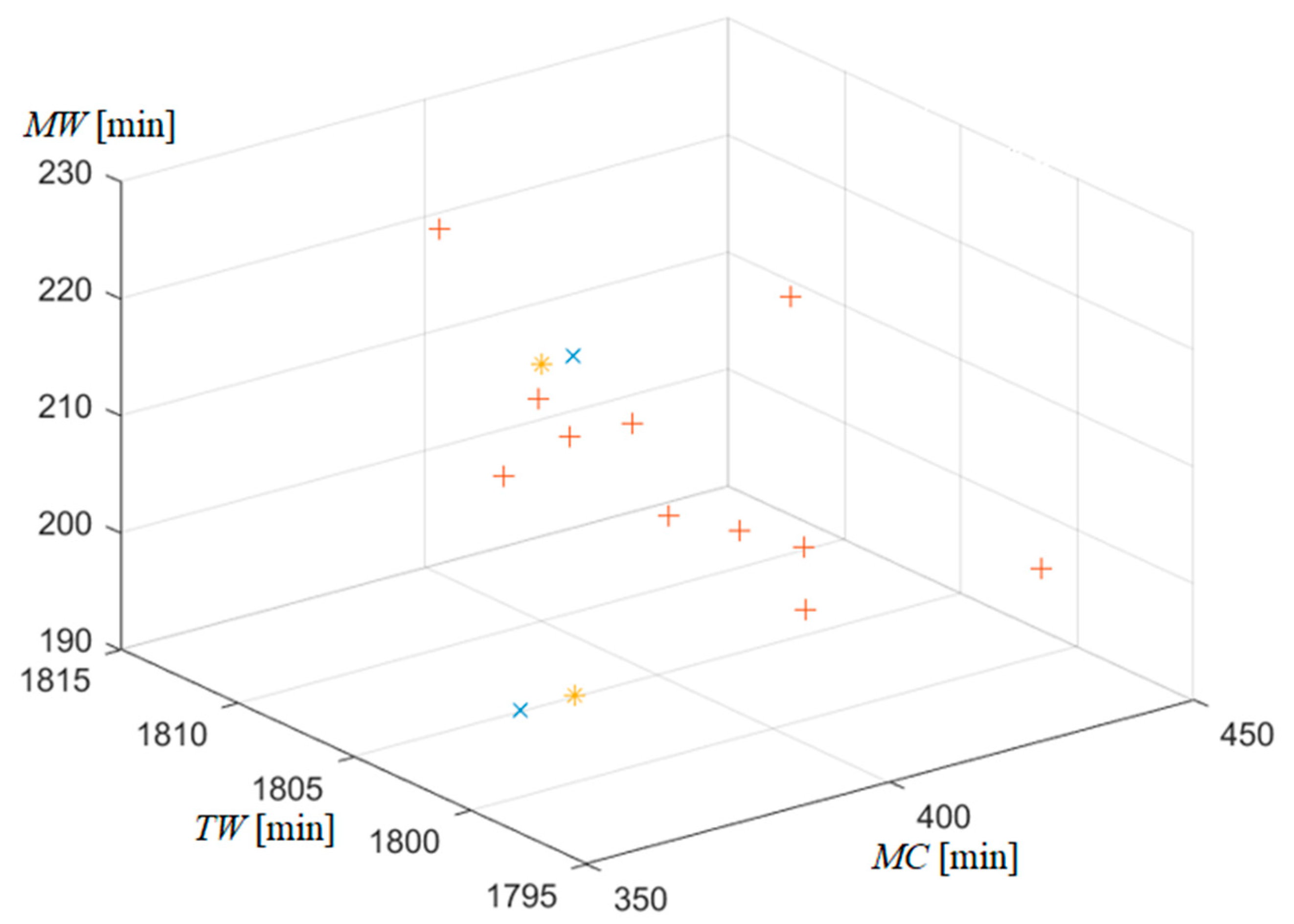
Figure 5 and
Table 11 shows the graphical and numerical optimization results of the three optimization algorithms, the proposed IHKA algorithm (mark
x) and the comparative two MOPSO (mark
*) and BBMOPSO (mark
+).
In order to prove the robustness of the optimization results, all three algorithms were tested in thirty interactions, and the average values of the optimization results are presented in
Table 11. Considering the graphical results shown in
Figure 5, we can conclude that the IHKA algorithm has proven to be the most appropriate for solving a real-world optimization problem. In its final interaction, it obtained the most optimal solution, which ensures the shortest makespan (MC) of orders and a consistent, high utilization of all machines (TW), without any bottlenecks in the manufacturing system (MW).
Optimization algorithms numerical results of the thirty interactions’ average values shows that the IHKA algorithm generated most optimal results at the two optimization parameters, at the orders’ makespan and the total machine utilization. In optimizing the machine utilization parameter of the most work loaded machine, the IHKA algorithm performed worst on average MW, in which parameter the BBMOPSO algorithm dominated. The IHKA algorithm compensated for the MW reduced ability to achieve the optimum result for the TW parameter, which is controlled by the appropriate scheduling of individual operations on the available machines.
The presented graphical and numerical results confirm the high capabilities and reliability of solving multi-criteria optimization problems of flexible manufacturing systems with the IHKA algorithm. The algorithm has been shown to be capable of solving complex optimization problems from a real-world environment.
Table 12 shows the example (for
J1 and
J2) of the IHKA output optimization results generated in the MATLAB software environment. The output optimization results of the optimization algorithm assign individual operation to the available machine, a start and finish time, and the machine sequence order in which it performs operations on the machine. The order of performing operations on the machine is performed according to the proposed method of its own decision logic [
26], which bypasses the integrated decision logic of the simulation environment. The automated transfer of numerical optimization results to the simulation environment allows the user to determine their own units of measurement according to the real-world manufacturing system.
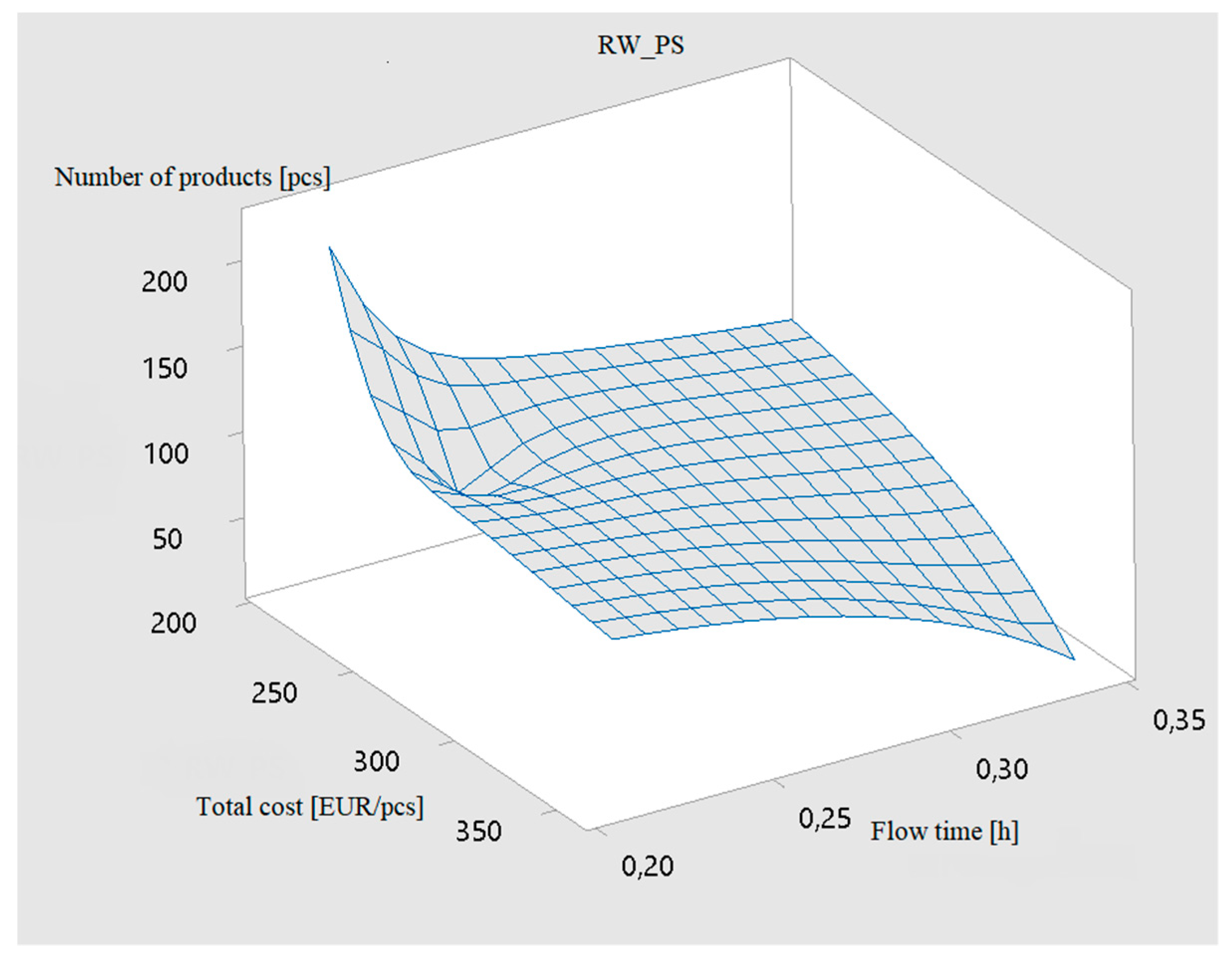
6.3. Validation of Optimisation Results Using the CTFP Diagram
In the stage of optimization results’ validation, an analysis of the optimization results was performed using the above presented CTFP diagram. Using the CTFP diagram, we can analyze the interdependence between three key parameters of flexible manufacturing systems: Time, costs and manufacturing flexibility interdependency. Manufacturing flexibility is defined using the previously defined approach in section five, where the mathematical distribution function was created to demonstrate the appropriateness of a new CTFP diagram method. For a simulation model of a real-world manufacturing system with fifteen orders and additional data that affect manufacturing flexibility, the values of the number of pieces in a single order product were determined with random function, from
Table 6 and
Table 7. With the introduction of the flexibility parameter, a dependency analysis was performed between the number of products, flow time and total order costs. The numerical results shown in
Table 13 and the graphical results shown in
Figure 6, show the optimization results’ correlation of the performed CTFP analysis between the Kacem 15 × 10, Mk10 test datasets and the RW_PS real production system dataset. All three datasets can be defined as high-dimensional cases, which means that a partial match is foreseen, especially in the graphical results that determine the typical CTFP format. It was found that the high-dimensional optimization problems of Kacem 15 × 10, Mk10 and the real-world manufacturing system dataset RW_PS show a significant dependence of the three mentioned parameters in ensuring production eligibility, while reducing production costs and shorter processing times significantly. The steep surface of the graph is particularly pronounced as the number of orders increases. The CTFP diagram in
Figure 6 shows that, by extending the flow time with a lower number of individual order products, this correlation affects the overall costs involved adversely. A well-optimized production process is crucial to ensuring the economic and process viability of custom production.
The impact of manufacturing flexibility on a sustainable production process is reflected in short flow times, high reliability of delivery due dates, low stocks, and a favorable cost-time profile linked to manufacturing flexibility and justified value stream architecture. These key production goals, which can only be achieved through appropriate multi-criteria optimization and additional objectives, are reflected in cost reduction through the rational and continuous use of workplaces, materials and machines, thereby ensuring a sustainably justified production system. With the help of graphical and numerical analysis of the CTFP diagram, we can see areas where the production system justifies the cost-time investment evenly, depending on the manufacturing flexibility. Based on the presented optimization approach, the company is able to adapt quickly to the global needs and demand of customers, while providing sustainable eligible production that increases total social and environmental benefits.
7. Conclusions
In the presented research work, we have presented the importance of a manufacturing flexibility and multi-criteria optimization method on the sustainable justified manufacturing systems. The initial research question was related to the ability to model manufacturing flexibility and its impact on cost-time investment, correlated with sustainable manufacturing processes, more sustainable products and social and environmental benefits [
2]. The main purpose of the research was to demonstrate a new approach to manufacturing flexibility modelling, based on a comprehensive consideration of all parameters with respect to a four-level architectural model [
13]. A mathematical method is presented for calculating the characteristics of a flexible job sop production system and determining the interdependencies between cost, time and manufacturing flexibility. A cost-time profile diagram and its impact on the production system are defined for the purpose of optimization results validation. Advantages and limitations are shown which relate to the ability to validate only single-criteria optimization problems. For the purpose of eliminating the shortcomings and extending the method, an experimental model based on the simulation scenario method is presented, which can be used to evaluate the impact of manufacturing flexibility on a sustainable justified production system. The optimization results are shown of multi-criteria optimization of five Kacem and Brandimarte test datasets [
24,
25] solved using the IHKA evolution method [
20] and the production adaptability modelling method. Based on the obtained numerical results, a graphical representation of the cost-time profile diagram influence on the manufacturing flexibility was performed, called the cost-time-flexibility profile diagram. The numerical and graphical results representation and validation are divided into three groups, according to the complexity of the solved problems (low, medium and high dimensional optimization problems). The validation approach presented here has advantages and limitations related to the three parameters of cost-time and manufacturing flexibility dependence, which are described and presented numerically and graphically.
In times of complex production systems, the transfer of theoretical methods to the real-world environment is especially important if we want to make our production systems sustainable. Therefore, an example is presented of an applied application of the proposed method to a medium-sized European high-mix low-volume manufacturing company. With the help of the proposed evolutionary computation method [
20], modelling of manufacturing flexibility and validation of cost-time investment, depending on the manufacturing flexibility, optimization and validation of the production system was performed, in order to define the sustainable orientation of the manufacturing company. Based on the numerical and graphical results, the IHKA evolutionary computational method best solved the multi-criteria optimization problem of a flexible job shop scheduling problem, represented by the RW_PS real-world dataset and evaluated by C-metric performance measures. The obtained optimization results make it possible to perform simulation modelling of the manufacturing flexibility impact on the cost-time investment. Using the simulation scenario method, a numerical analysis of the manufacturing flexibility impact on the optimization parameters was performed, which affected the sustainability of the production system critically. Based on the presented method, we find that it serves companies in order to optimize existing manufacturing systems and to construct or design new manufacturing systems optimally, in order to correlate costs, time and manufacturing flexibility properly. Adequate CTFP ensures sustainable production from the energy and natural resource consumption, equal workload of workers and machines, improvement of product quality and customer satisfaction point of view. By achieving a balanced CTFP chart, we ensure sustainable business growth, and provide increases in a company’s total, social and environmental, benefits.
The presented research work has limitations that relate to the evaluation and modelling of the presented method solely for flexible job shop types of manufacturing systems. At the same time, using the cost-time profile diagram, it can evaluate just about every production system. It should be emphasized that the impact of manufacturing flexibility is the most significant in the devalued type of production, and is more difficult, or even not present, in other types of production (mass production, etc.). In order to ensure the robustness of the proposed CTFP diagram approach, it would be appropriate to transfer and evaluate it to other production types in order to ensure the wide applicability of the proposed method.
The presented methods and results of mathematical and simulation modelling in correlation with the methods of defining cost-time investment and their correlation with the manufacturing flexibility, and multi-criteria optimization using IHKA optimization method, provide sustainably and financially justified production systems. Compared to the results of other researchers evaluating dynamic, flexible manufacturing systems and different decision models, the presented manuscript deals with the meaning of multi-criteria optimization of production system scheduling. The considered research case is formulated mathematically with the input parameters covering the majority of characteristics of production systems (makespan, process time, setup time, operational costs, idle costs, energy cost, order quantity, machine power, etc.). The optimization parameters are divided into three groups regarding the machine classification, based on which it is possible to describe the manufacturing system in detail using evolutionary computation methods, to allocate the work orders optimally to the appropriate, available highly-utilized machine. The presented comprehensive optimization method enables both numerical and graphical representation of optimization results. The modular structure enables interaction between the IHKA decision model, the simulation model and the graphical CTFP representation of the optimization results by means of cost-time investment, depending on manufacturing flexibility. Of course, devoting to optimizing only the FJSSP production type, for example with other researchers [
28], is a limitation. Given that, other research focuses on demonstrating the impact of flexible line redesign planning problems [
28] and determining the impact of the market uncertainty [
29] on the adaptability and feasibility of using flexible and dedicated machines on the occupancy of manufacturing utilization using the Monte Carlo simulation method. The presented research work represents the originality with the economical and sustainable optimization approach. Other research works cite as a complexity a very wide range of optimization parameters that need to be defined properly mathematically, and their interdependence must be described; that limitation is well presented in described research work. The presented research work is, thus, an original contribution, with a comprehensive multi-criteria optimization approach and associated simulation modelling methods, using the simulation scenario approach, graphical and numerical definitions of optimization results by means of cost-time investment depending on manufacturing flexibility. The holistic approach is rounded off by an appropriately sustainable and economically justified method for ensuring optimized, highly flexible manufacturing processes that are increasingly present in the current era of Industry 4.0.
Thus, this research represents the basic research work for the further development of the manufacturing flexibility dependence on cost-time investment and, consequently, on sustainable orientation manufacturing systems. The influence of different parameters and, thus, solving multi-criteria optimization problems is crucial in ensuring economically, socially and environmentally sustainable production systems, which is defined clearly in this research work. The presented importance of optimizing highly flexible manufacturing systems opens up many possibilities for further research work. The introduction of collaborative workplaces into production systems represents a new research area, where the flexibility of collaborative robots allows high adaptability of manufacturing capacities with respect to the ability to perform different operations at different workplaces. The introduction of highly flexible workplaces also increases the complexity of multi-criteria optimization problems, that can be solved using the proposed evolutionary computation methods. Consideration of the feasibility of introducing and implementing collaborative workplaces from the economic and sustainable eligibility point view has not yet been investigated. Further research and implementation of the presented methods will allow evaluation of the justification for the introduction of the highly flexible workplaces in different types of production systems, thus ensuring optimized, sustainable and economically viable production systems.


