Article

Location Optimization of CR Express International Logistics Centers

1
Department of Transportation Engineering, School of Naval Architecture, Ocean and Civil Engineering and State Key Laboratory of Ocean Engineering, Shanghai Jiao Tong University, Dongchuan Road 800, Shanghai 200240, China
2
Department of Logistics and Transportation Systems Management, Mining Engineering and Transport Institute, Nosov Magnitogorsk State Technical University, Lenina Street 38, 455000 Magnitogorsk, Russia
3
Sino-US Global Logistics Institute, Shanghai Jiao Tong University, Huashan Road 1954, Shanghai 200030, China
4
Department of Logistics, University of Defence in Belgrade, Pavla Jurišića Šturma 33, 11000 Belgrade, Serbia
*
Author to whom correspondence should be addressed.
Symmetry 2020, 12(1), 143; https://doi.org/10.3390/sym12010143
Submission received: 6 December 2019 / Revised: 31 December 2019 / Accepted: 7 January 2020 / Published: 10 January 2020

Abstract

:
Currently, the trade volume between China and the European Union is experiencing rapid growth. However, there are many bottlenecks in the operation of the China Railway Express, such as imbalance in inbound and outbound transported containers in the Sino–European direction and a low profit margin. More than fifty-three rail routes in China provide rail transportation to European cities and have small traffic volumes. However, such a dramatic situation affects transportation costs, which are three times higher compared with maritime transportation, causing uncertainty related to the demand of Chinese customers. This study analyzes the shortcomings of previous research studies related to multicriteria decision-making (MCDM) models applied in the field of logistics and transportation. The study proposes a novel approach to determine the optimal locations of the CR Express international logistics centers. The proposed approach involves the application of a MCDM model using the DEMATEL-MAIRCA method. This technique finds the closest solution to the ideal one by identifying the value of the best alternative in line with the observed criterion, and by measuring the distances of other alternatives according to the observed criterion of the ideal value. Finally, we show the similarity of the proposed methodology to other MCMD methods, which is one of the key topics of the Symmetry Journal, to prove the validity of the applied DEMATEL-MAIRCA method. Preliminary results show that in view of increased container turnover between China and the European Union, the determination of optimal locations for CR Express international logistics centers should be carried out dynamically.

1. Introduction

Currently, the trade market between China and European countries in the framework of the “One Belt, One Road” initiative has been rapidly developing. According to experts’ forecasts, the number of containers will be increased by 800,000 TEU’s in 2020, which is five times more than in 2015.
The main actor providing rail transportation between China and European countries is the China Railway express (CR Express). Despite efforts from governments and enterprises in both China and the countries along the route, the number of blocked trains and containers has increased dramatically in the last six years. By the end of March 2019, the total number of operations on the CR Express had exceeded 7600 round trips, and the number of domestic routes in China had reached 61 across 43 cities, which are the current international logistics centers. The CR Express operates in 41 cities across 13 countries in Europe [1].
Undoubtedly, the CR Express has been developing rapidly in recent years. However, the high rail transportation costs between China and the European Union have a negative impact on the demand for this transportation method. By the end of 2017, the average price had dropped from 9000 $/TEU to 6000 $/TEU on average, which is still much higher than maritime transportation. Furthermore, the volume of the goods that European countries deliver to China by railway is comparatively small. In 2017, the number of trains from Europe to China was 67% of the number from China to Europe, meaning that operators cannot make full use of the containers, and the profit of whole transportation process is limited [1]. Therefore, most of the companies that run the CR Express are suffering losses, depending on the subsidies from local governments, which leads to competition for subsidies between different provinces in China. Finally, to date, almost every Chinese city running the CR Express has chosen to set up their own route by themselves. This has caused a lack of holistic planning and route combinations, increasing the total expense of the CR Express operation.
To solve the problem of high transportation costs, it is imperative to optimize the railway service network, particularly the optimal location of international logistics centers. There are several reasons to select the optimal location of international logistics centers and minimize the number of rail routes by reducing the number of cities. Firstly, freight transportation flows could be aggregated and economies of scale could be achieved. Secondly, it could potentially increase the volume per single trip, which would allow Chinese companies to charge more when collaborating companies along the routes. Finally, it could reduce transportation costs, avoid inefficient routes, and improve operation efficiency. If the transportation cost can be cut down, fewer subsidies from the government will be needed for transportation companies, which will decrease the burden on the government and increase the motivation of market players.
To date, several studies have been conducted on the facility location problem (FLP), including case studies on the CR Express, which are mainly focused on the application of multicriteria decision-making methods (MCDM) [2,3] or a combination of MCDM methods and deterministic optimization models [4,5].
However, these studies have several limitations. Firstly, the authors consider a limited number of criteria affecting the selection of the optimal logistics center locations, since these facilities are complex. This means that those facilities consist of many elements, the parameters of which are affected by different external factors. Consequently, this causes inaccuracy in the results. Secondly, most of the applied MCDM methods used to solve facility location problems are unstable in alternative rankings, sensitive to inconsistent data, difficult to develop, and based on experts’ opinions.
The contribution of this paper can be summarized as follows. Firstly, this work reviews the existing and relevant literature for various MCDM methods with regard to transportation and logistics. Secondly, this work presents the hybrid multicriteria decision-making DEMATEL-MAIRCA model, which is used to select the optimal location of the CR Express international logistics centers (CILC). The decision-making trial and evaluation laboratory (DEMATEL) method is based on collective judgment and is used to identify the cause–effect relationships among selected strategic criteria in order to select precandidate cities for CILC. The multiatributive ideal-real comparative analysis (MAIRCA) method aims to compare the conceptual and experimental alternative ratings, and is able to estimate the alternatives and select precandidate cities for CILC. Additionally, a case study on CILC selection is presented. Lastly, the paper provides critical managerial insights for different decision makers, such as logistics managers and local government.
The remainder of this paper is structured as follows. Section two provides a review of the relevant literature. The third section introduces the description of the applied DEMATEL-MAIRCA methodology. The fourth section presents a case study on the selection of precandidate cities for CR Express international logistics centers. The fifth section provides a comparison between the proposed methodology and other modern MCDM techniques. Finally, this paper summarizes future development strategies for designing an optimal railway network for CR Express international logistics centers.

2. Literature Review

The methods employed in existing studies related to the facility location problem can be primarily grouped into two categories: quantitative mathematical methods and mathematical programming techniques. With respect to the facility location problem, the MCDM methods are often utilized for developing the ranking of potential locations based on expert opinions. Bridgman published the first paper on the MCDM method based on the weighted product model (WPM). This method relies on the comparison between alternatives through the multiplication of the ratio number (one for each criterion) [6]. Since then, the proposed technique has attracted the attention of many other researchers, which has improved the mentioned method. Fishburn proposed the weighted sum model (WSM) for solving the issues associated with the identical physical dimensions of studied variables. In other words, this method comprises the application of the “additive utility” assumption [7]. However, this method is not able to solve the problems related to various distinct types of criteria and variables [8]. Saaty presented an analytical hierarchy process (AHP), which relies on investigating priorities or weights of importance among the selected criteria and alternatives. However, the possible compensation between positive and negative scores for some criteria could cause information failure [9]. Furthermore, the implementation of the proposed method is inconvenient due to the technique’s complexity. Roy proposed the elimination and choice expressing reality (ELECTRE) method based on partial aggregation. This method attempts to rank alternatives with respect to a concordance and discordance index, which is calculated through obtaining data from a decision table [10]. However, this method involves an additional boundary value, and the rating of the alternative is determined based on the size of this boundary value, which does not contain the correct value [11].
Further studies have focused on improving the MCDM method. The improved ELECTRE III/IV method was implemented to select the optimal location of a logistics center in Poland [3]. This method uses binary outranking relationships. The dataset applied in this method consists a final set of alternatives, a family of criteria, and preferences offered by decision makers [12]. However, this method is time consuming, since it requires sophisticated application and probable incapability to identify a preferred solution [13].
The multicriteria optimization and compromise solution (VIKOR) technique was used to select the optimal location of a distribution center for security materials. This method uses inconsistent and incommensurable (attributes with different units) criteria. This means that a compromise solution can be achieved for conflict resolution while the decision-maker aims to find a solution that is the closest to the ideal one. Furthermore, the alternatives can be estimated in line with the established criteria [14]. Nevertheless, this method has numerous limitations, such as the need to correlate criteria, the uncertainty of the weights obtained using only objective and subjective methods, and the option of an alternative being close to the ideal point and nadir point at the same time [15].
Atanassov interval-valued intuitionistic fuzzy sets (AIVIFS) were applied to select the location of a production plant in Serbia [16]. This methodology is based on the values of its membership and nonmembership functions, which are represented as intervals instead of exact numbers [17]. However, this method uses max–min–max composition losses of information, because the composition neglects most values except for extreme ones [18].
The SWARA-WASPAS method was used to select the optimal location of a shopping mall in Iran [19]. The idea of a step-wise weight assessment ratio analysis (SWARA) involves the determination of relative importance through the inputs provided by experts [20]. The weighted aggregated sum product assessment (WASPAS) method is based on the combination of a weighted sum model (WSM) and weighted product model (WPM) [21]. Nevertheless, the WASPAS method has several drawbacks, such as the unbalanced increase in the value of the objective function as a result of linear WPM function. This is significant for the initial decision matrix, which contains the boundary values of the individual elements [22].
The combination of evaluation based on the distance from the average solution (EDAS) and weighted aggregated sum product assessment with normalization (WASPAS-N) methods was applied to select a teahouse location in China [23]. The EDAS method obtains the best alternative related to the distance from the average solution [24]. The WASPAS-N method aggregates the normalized values of the decision matrix by applying the weighting related to the criteria involving arithmetic and geometric means [25]. Nevertheless, the EDAS method cannot be applied in stochastic MCDM problems involving different distribution laws.
The fuzzy technique for order of preference by similarity to ideal solution (TOPSIS) was used to select the optimal locations of shopping malls in Turkey [26]. This method selects the alternatives that have the shortest distance from the positive ideal solution and the farthest distance from the negative ideal solution at the same time [27,28]. However, it requires numeric attribute values that monotonically increase or decrease and have comparable units that could potentially complicate the data collection [29].
The combination of the TOPSIS technique and multichoice goal programming (MCGP) was applied to select the optimal location of a logistics center for the airline industry [30]. The concept of the proposed combination lies in the implementation of the obtained criteria weights using TOPSIS into each goal of MCGP. The idea of the MCGP methodology is based on the application of multiple aspiration levels for their problems, where these levels are categorized as “more appropriate” or “less appropriate” [31]. However, if each objective’s aspiration level is represented by the continuous decision variable, which could range between lower and upper bounds, this approach does not provide the option for decision makers to control the bounds of the interval aspiration level [32].
The fuzzy data envelopment analysis (DEA) method was proposed to predict the results and efficiency of alternative control actions for train dispatchers to prevent potential disturbances on a railway line [33]. This nonparametric method analyzes the relative efficiency of decision-making units (DMUs) based on numerous inputs and outputs [34]. Nevertheless, this method is inadequate in ranking efficient DMUs with fuzzy numbers, and it is based on the self-evaluation of DMUs [35].
To overcome the shortcomings of the reviewed studies in the field of FLP and provide a case study, we propose the application of the DEMATEL–MAIRCA method. Since various diverse factors affecting the locations of logistics facilities mean the FLP is a multidisciplinary problem requiring a complex selection procedure, we propose the application of the MCDM method. This will make it possible to select the potential precandidate cities for the international logistics centers in China.

3. The Hybrid DEMATEL-MAIRCA Model and Case Study

The proposed DEMATEL–MAIRCA model was developed by Serbian researcher Dr. Dragan S. Pamucar [36]. The application of the MCDM model is a hybrid of two techniques. The fuzzy DEMATEL model collects knowledge to capture the causal relationships between strategic criteria [37,38]. The model is especially practical and useful for visualizing the structure of complicated causal relationships with matrices or digraphs [39,40]. In other words, this method would identify the causal relationship among the selected criteria. The multiattribute ideal–real comparative analysis (MAIRCA) compares both theoretical and empirical alternative ratings [41], evaluates the alternatives, and selects precandidate cities for allocating CILC. The phases of the DEMATEL-MAIRCA method are presented in
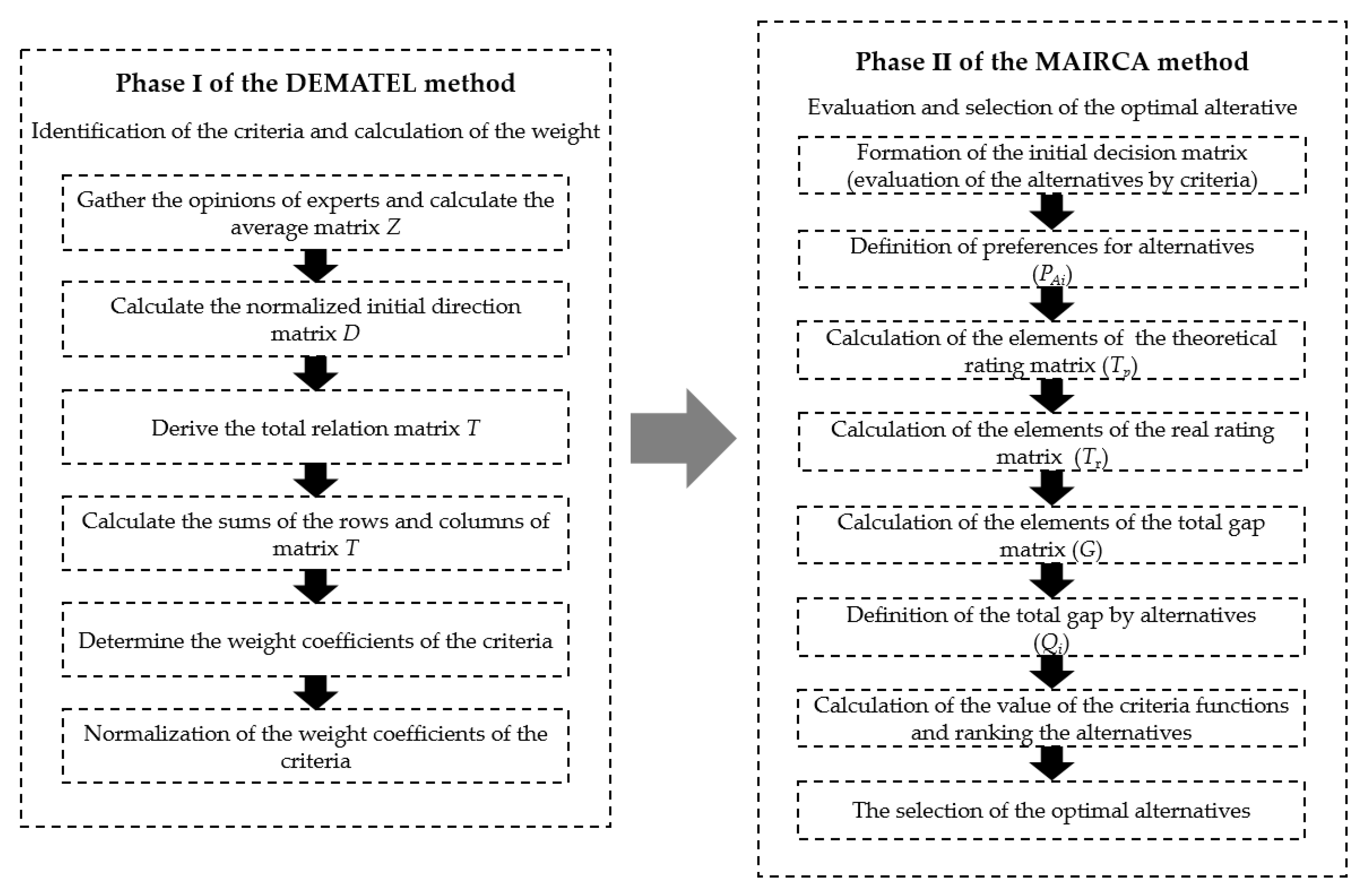
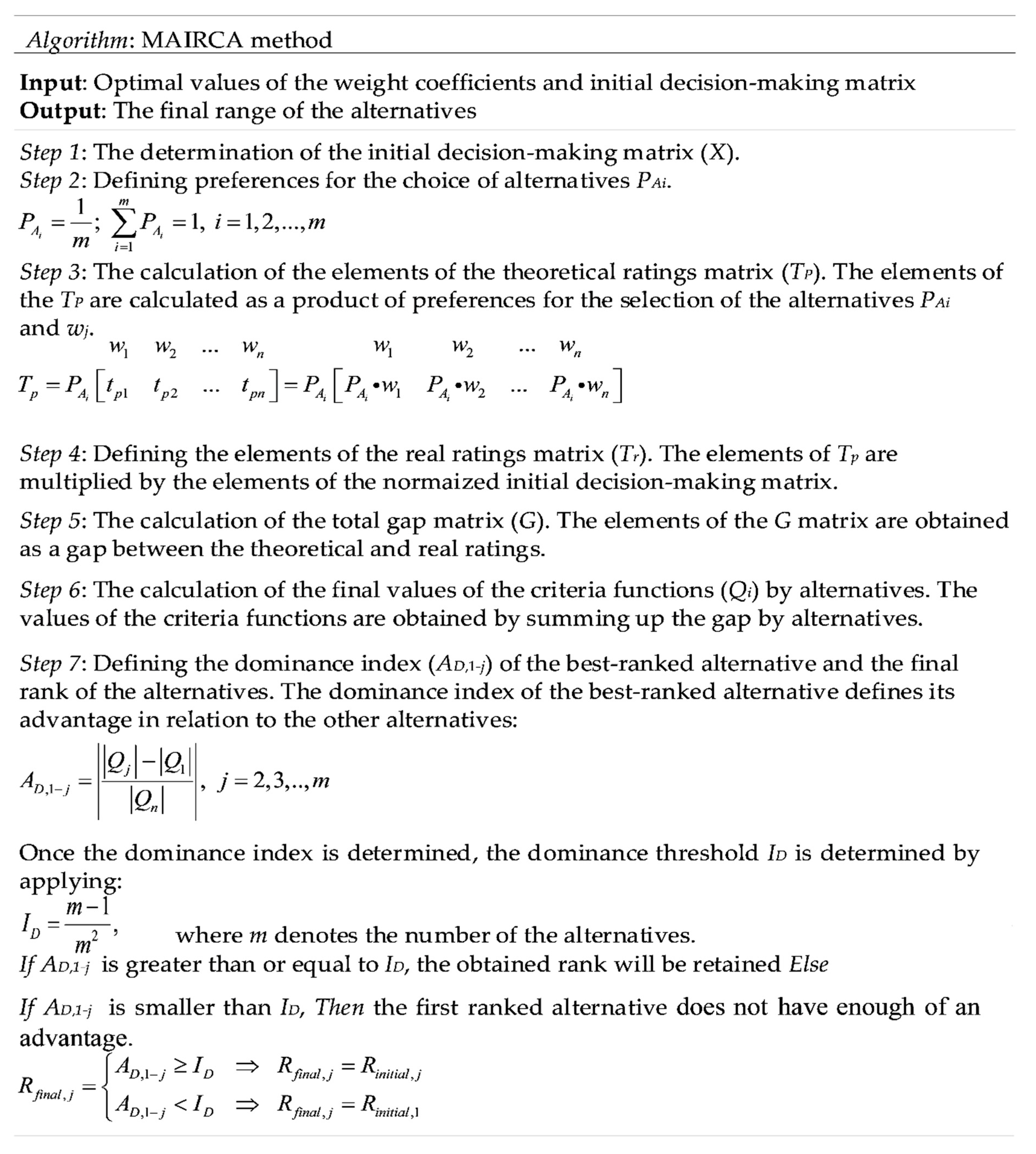
 Figure 1.
Pamucar proved that the proposed method provides lower instability in alternative rankings compared with traditional methods [36]. Moreover, the application of the MAIRCA model has several advantages. Firstly, this method has greater stability compared with other methods, such as TOPSIS or ELECTRE [36]. Firstly, this technique provides a different criteria normalization method. It has been proven that MCDM techniques apply a linear model of input data normalization that is more stable and ranks constantly in the sensitivity analysis. Secondly, the MAIRCA method is simpler from a mathematical perspective. It also provides solution stability and can be hybridized with other MCDM techniques [2]. In order to determine the causal relationship among the selected criteria, we propose the application of the fuzzy DEMATEL method.
Essentially, we aim to select precandidate Chinese cities, which should be evaluated and compared with each other based on the selected criteria. The alternatives are assigned as vectors. Each vector represents the value of the i-th alternative by the j-th criterion. Since the variable of the criteria affects the final ranking of alternatives, each criterion is presented as a weight ratio. This effect considers its relative value in estimating the alternatives. Since we need to establish the relationships among the criteria, the fuzzy DEMATEL method is applied. The algorithm of the fuzzy DEMATEL method is presented in Figure 2.
The first step was the collection of the expert scores and calculation of the average matrix Z. This step involved the evaluation of the impact level between selected criteria by participating experts. Each expert’s opinion is represented as a non-negative matrix. The impacts of the criteria on each other are expressed by linguistic expressions. In order to list the pairwise comparisons, linguistic expressions using triangular fuzzy numbers are applied. Finally, all experts’ opinions are aggregated into the average matrix Z.
Since we calculated the elements of the matrix Z, we could determine the elements of the normalized initial direct relation matrix D. The elements of the D matrix are determined by summing the elements of the average matrix Z by row. The next step revealed the finalization of matrix elements T by summing rows and columns. The separate summarization of both rows and columns in the sub-matrices T1, T2, and T3 is represented by the fuzzy numbers Di and Ri. Since we obtained the Di and Ri values, the criterion weights were calculated using the obtained fuzzy value of the weight coefficients. In order to facilitate the normalization of weight coefficients, the defuzzified value of the weight coefficients was applied prior to normalization.
To obtain the weights of the selected criteria, we applied the MAIRCA model. The purpose of the MAIRCA model is to evaluate the gap between ideal and empirical ratings. To identify the total gap for each alternative, we needed to sum the gaps in each criterion. Finally, the ranking of the alternatives could be obtained, where the best-ranked alternative contained the smallest gap value. The alternatives with the smallest total gap values were close to the ideal ratings. To solve a decision problem by applying the MAIRCA method after determining alternatives and related criteria, the following steps are validated. The algorithm of the MAIRCA method is presented in Figure 3.
The first step presents the formulation of the initial decision-making matrix X. This matrix analyzes the criteria values for each alternative. The criteria of matrix X could be quantitative or qualitative. The quantitative values of the criteria in the matrix X are determined by quantifying the real indicators among the selected criteria. The qualitative values of the criteria are obtained by choices made by the decision makers. If the study has a large number of experts, we propose to aggregate the opinions of the experts.
The second step estimates the preferences to select the alternatives. This selection is based on indifferent decision makers’ opinions. This means that there is no preference for selected alternatives. Moreover, the decision maker is indifferent in both selecting any specific alternative and in the process of the alternatives’ selection.
The third step reveals the computation of the theoretical ratings matrix Tp. The matrix Tp is represented as the multiplication of the total number of criteria and the total number of alternatives. The theoretical ratings matrix is calculated by multiplying preferences to select the alternatives and criterion weights. These decision-maker preferences are the same for all alternatives, since they are indifferent in the initial selection of the alternatives.
The calculation of the real ratings matrix Tr involves multiplying the elements of the theoretical ratings matrix Tp and the elements of the initial decision-making matrix X.
The fifth step involves calculating the total gap matrix G. The G matrix is calculated as the difference between the theoretical and real ratings. In other words, it is the gap between the theoretical ratings matrix Tp and the real ratings matrix Tr.
The sixth and seventh steps obtain the final values of criteria function Qi by alternative and the final alternative ranking methods. In order to obtain the values of criteria functions, we propose summing the gap with the alternatives. In other words, we should sum the elements of G matrix by column.

4. Case Study

To identify the criteria selected in affecting the CILC location [3,42] and presented in Table 1, we have provided interviews with international logistics companies, local government, and surveys with scholars in the field of logistics, supply chain management, and transportation.
The preliminary selection of the potential precandidate cities is based on conducted research presented in [4], such as cities in which the CR Express already operates, cities that have been selected for further development by Chinese national strategic policy, and capital cities of provinces. The selected potential precandidate cities are Guangzhou, Changchun, Changsha, Chengdu, Chongqing, Guiyang, Harbin, Hefei, Hohbot, Kunming, Lanzhou, Liuzhou, Nanchang, Ningbo, Qingdao, Shanghai, Shenyang, Shijiazhuang, Suzhou, Taiyuan, Tianjin, Urumqi, Wuhan, Xiamen, Xi’an, Yinchuan, and Zhengzhou.
The initial step of the DEMATEL method involves applying the triangular fuzzy scale presented in Table 2 to evaluate the impacts between criteria.
The compiled surveys created eight average matrices. The preferences of experts were collected into an average matrix Z. Then, we obtained Table A1. The elements of the initial direct relation matrix D are normalized by dividing each element of the matrix Z by the maximum element among the summed experts’ opinion.
In order to derive Table 3, the elements of matrix T illustrated in Table 2 are summed by rows and columns.
Table A2 demonstrates the aggregated values of matrix T by rows (Di), columns (Ri), and the obtained weights of each criterion (wi). Then, we estimated the alternatives in Table A4 and selected them by applying the MAIRCA method. In order to estimate the alternatives by using the qualitative criteria, we applied the linguistic fuzzy scale.
Table A4 presents the criteria, which is categorized in the following way. Max is related to profit-type criteria, where the highest values are favored. Min is associated with the cost-type criteria, characterized by the lowest values (which are also favored). Since we formulated the initial decision-making matrix in Table A5, the preferences of experts for the selected alternatives PAi are obtained by the formula PAi = 1/m = 1/27 = 0.037, where m is the total number of potential precandidate cities. Then, the elements of the theoretical ratings matrix (Tp) are calculated:
t p 42   =   P A 4   ·   w 2   =   0.037   ·   0.060   =   0.00198
As the theoretical ratings matrix (Tp) has been derived, we can calculate the real ratings matrix (Tr). The elements of the real ratings matrix presented in Table A6 are obtained by multiplication of the elements presented in the theoretical ratings matrix (Tp) and normalized elements of the initial decision-making matrix (X). For example, the position tr32, which is the element of the real ratings matrix, is obtained with the following formula:
t r 42   =   t pij   ·   ( x ij     x i x i +     x i ) =   0.00198   ·   ( 5151.59     4209.28 9860.00     4209.28 )   =   0.00033
The elements of the total gap matrix (G) presented in Table A7 are calculated as the difference (gap) between theoretical ratings (tpij) and real ratings (trij). The element of the total gap matrix at position g42 is determined with the following formula:
g 42   =   t p 42     t r 42   =   0.00198     0.00033   =   0.00165
The gap for the alternative A4 with the criterion U2 is g42 = 0.00165. Regarding criterion U2, the obtained ideal alternative is dependent on tpi2 = tri2 (i.e., gi2 = 0:00). In order to evaluate the unideal alternative with criterion U2, the condition is tri2 = 0 (i.e., gi2 = tpi2). Consequently, evaluating the alternative A4 with criterion U2, is not the ideal alternative (Ai+). Furthermore, alternative A4 is closer to the ideal alternative as compared to the unideal alternative, since the distance from the ideal alternative is g42 = 0:0084.
To obtain the values of criteria functions (Qi) using alternatives presented in Table 3, we summed the gaps (gij) with the alternatives. In other words, we summed the elements of matrix (G) by columns; the alternative should preferably have the lowest possible value of the total gap (in this case, alternative no. 27).
The presented methodology allows us to select the precandidate cities for the CR Express international logistics centers. One of the key features of the applied method is the ability to scale the model, since a large number of criteria with different units were applied. Moreover, this method is very useful for different stakeholders, such as logistics managers and local government, since it is capable of handling large-scale problems and can produce infinite alternatives. Finally, the calculation is simple and does not require complex computer programs.
The preliminary results presented in Table 3 illustrate that the number of cities and their order are both changed. Figure 4 demonstrates that three areas have less precandidate cities after the applied methodology. Next, we will investigate the reduced number of cities from different perspectives.
Firstly, from the infrastructure point of view, the reduced number of cities could potentially improve the throughput of the specific CR Express rail routes and access roads among the CILC. Moreover, as the optimized number of cities assumes increased traffic volumes, industrial enterprises should be located closer to CILC. In other words, we assume the rapid development of the industry.
Secondly, from the social and economic perspectives, the optimal number of cities could reduce the amount of the subsidies provided by the local government for development of the logistics infrastructure. This means that local authorities could forward the cash flow and use it to develop other sectors, such as healthcare and education. Furthermore, since the reduced number of cities implies increased traffic volumes, this could potentially increase the workforce and salaries of CILC workers.
Finally, in view of increasing environmental requirements in China, the optimized number of cities minimizes the volume of the solid waste produced by the CILC, the CO2 emission produced by trucks, servicing requirements for the CILC, as well as reduces noise pollution by reducing the amount of technological equipment in operation at the CILC. In addition, the number of lost containers could be reduced, since having a minimized number of cities reducers containers’ movements.

5. Comparison and Discussion

In the previous section, we showed the applicability of the DEMATEL-MAIRCA method for solving the facility location problem. However, in order to prove the validity of the proposed methodology, we will compare this method with other modern methodologies, such as multiobjective optimization on the basis of ratio analysis (MOORA), complex proportional assessment (COPRAS), and multiattribute border approximation area comparison (MABAC) methods.
The MABAC method was firstly formulated by Pamucar and Cirovic in 2015 [43]. This method computes the distance between each alternative and the bored approximation area (BAA) [44,45].
The COPRAS method was developed by Zavadskas, Kaklauskas, and Sarka in 1994. This method compares the alternatives and determines their priorities under the conflicting criteria by taking into account the criteria weights [46].
The MOORA method was firstly introduced by Brauers in 2004 [47]. This method involves multicriteria or multiattribute optimization and allows simultaneous optimization of two or more conflicting attributes (objectives) subject to certain constraints.
Based on computational experiments, we obtained the following alternative rankings and provided a correlation between the DEMATEL-MAIRCA method and other methods presented in Table 4. In order to compare the results obtained by the four different approaches (Table 4), we used Kendall’s tau correlation coefficient. Kendall’s tau correlation coefficient (KTC) of ranks is a valuable and significant indicator for investigating the relation between the obtained results from the applied four different approaches [24]. Moreover, the KTC is useful when a study contains ordinal variables or ranked variables, which is relevant in the present case. It also has been proven that KTC is more stable and more efficient than Spearman’s rank correlation (SCC) [48]. The KTC was applied in the present study to determine the statistical difference of importance among the obtained ranks. The correlation between the DEMATEL-MAIRCA method and other methodologies is presented in Table 4.
From the total calculated statistical coefficient of correlation (0.987), we conclude that the obtained ranks have a high correlation with each other. All the KTC values are greater than 0.90, which according to Ziemba [49] illustrates high correlation. In Table 4, all of the KTC values are considerably greater than 0.90, with an average value of 0.984. This means that there is a high correlation between the proposed DEMATEL-MAIRCA method and the other MCDM techniques. It can be concluded that the obtained ranking is acceptable and reliable. In other words, the provided comparison proves that the proposed methodology is adequate and valid.

6. Conclusions

This study presents the application of the hybrid DEMATEL-MAIRCA model to select the optimal locations of CILC. The DEMATEL method was applied to identify the weights of the criteria. The MAIRCA method was applied to evaluate the alternatives and select the locations of precandidate cities for CILC.
The main advantage of the applied methodology is its universality, since this method could be applied to other decision-making problems involving MCDM methods. Moreover, the applied technique could be applied in the case of a large number of alternatives and criteria. Furthermore, it clearly ranks the numerical values, allowing an easier understanding of results, and could be applied qualitative and quantitative types of criteria. Finally, the proposed method is robust; the DEMATEL-MAIRCA method is more stable in conditions of risk and uncertainty compared with other techniques. This means that the method is less sensitive to changes in the weights of selected criteria and related changes in alternative ranking.
The applied methodology is a practical tool for different stakeholders, such as logistics managers and local government. On the one hand, the ranking of the cities provides the possibility of finding optimal CILC locations and reduces rail transportation costs. On the other hand, it also affects the environmental aspects [50], since the number of potential precandidate cities is minimized. The case study shows the difference between the current CR Express railway network in China and the obtained optimal network. The obtained optimal CR Express railway network includes precandidate cities in areas where the freight transportation flows can be aggregated and economies of scale can be achieved. The provided comparison between the proposed methodology and other MCDM techniques shows a strong correlation, which demonstrates the validity of the DEMATEL-MAIRCA method.
Several limitations should be considered. Firstly, since the present study aggregates experts’ opinions, data triangulation should be provided to investigate the impacts of different criteria. Secondly, as there has been an imbalance in cargo flow between China and Europe, the criterion related to Chinese customers’ demand for the CR Express service should be considered. Finally, in order to provide a comprehensive study, the same proposed approach should be applied to select the optimal location of CILC in Europe.
Further development of the study should include the application of the selected precandidate cities for the design of an optimal railway network between China and Europe. In order to design the optimal railway network, we propose the development of a mixed-integer mathematical model that would be applied in the AnyLogistix software. This software is based on supply chain optimization. By using the proposed software and scenario approaches, and including stochastic variables such as demand and transportation time, an optimal CR Express railway network can be designed.

Author Contributions

Conceptualization, D.M., H.H. and D.P.; methodology, D.M. and D.P.; validation, D.M., H.Z. and D.P.; investigation, D.M. and H.Z.; data curation, D.M. and H.Z.; writing—original draft preparation, D.M., H.H., H.Z. and D.P.; writing—review and editing, D.M., H.H., H.Z. and D.P.; visualization, D.M., H.Z. and D.P. All authors have read and agreed to the published version of the manuscript.

Funding

This research received no external funding.

Conflicts of Interest

The authors declare no conflict of interest.

Appendix A

Table A1. Average matrix (Z).
ZijU1U2U3U4U5U6U7U8U9U10U11U12U13U14U15U16U17
U1(0.00, 0.00, 0.00)(0.20, 0.47, 0.80)(0.80, 0.80, 0.80)(0.40, 0.67, 0.80)(0.80.0.80.0.80)(0.20, 0.50, 0.80)(0.40, 0.60, 0.80)(0.20, 0.50, 0.80)(0.60, 0.70, 0.80)(0.80, 0.80, 0.80)(0.60, 0.70, 0.80)(0.80, 0.80, 0.80)(0.80, 0.80, 0.80)(0.60, 0.70, 0.80)(0.80, 0.80, 0.80)(0.20, 0.50, 0.80)(0.20, 0.20, 0.20)
U2(0.80, 0.86, 1.00)(0.00, 0.00, 0.00)(0.80, 0.80, 0.80)(0.20, 0.53, 0.80)(0.80.0.80.0.80)(0.20, 0.50, 0.80)(0.40, 0.60, 0.80)(0.40, 0.53, 0.80)(0.20, 0.50, 0.80)(0.80, 0.80, 0.80)(0.40, 0.60, 0.80)(0.40, 0.60, 0.80)(0.80, 0.80, 0.80)(0.20, 0.50, 0.80)(0.20, 0.50, 0.80)(0.20, 0.50, 0.80)(0.20, 0.20, 0.20)
U3(0.80, 0.80, 0.80)(0.60, 0.73, 0.80)(0.00, 0.00, 0.00)(0.20, 0.50, 0.80)(0.60, 0.70, 0.80)(0.20, 0.50, 0.80)(0.60, 0.70, 0.80)(0.60, 0.67, 0.80)(0.20, 0.50, 0.80)(0.80, 0.80, 0.80)(0.60, 0.70, 0.80)(0.80, 0.80, 0.80)(0.80, 0.80, 0.80)(0.20, 0.50, 0.80)(0.20, 0.50, 0.80)(0.20, 0.50, 0.80)(0.20, 0.20, 0.20)
U4(0.60, 0.80, 1.00)(0.60, 0.67, 0.80)(0.80, 0.80, 0.80)(0.00, 0.00, 0.00)(0.60, 0.70, 0.80)(0.60, 0.70, 0.80)(0.80, 0.80, 0.80)(0.80, 0.80, 0.80)(0.80, 0.80, 0.80)(0.80, 0.80, 0.80)(0.80, 0.90, 1.00)(0.80, 0.90, 1.00)(0.80, 0.80, 0.80)(0.80, 0.90, 1.00)(0.20, 0.50, 0.80)(0.80, 0.90, 1.00)(1.00, 1.00, 1.00)
U5(0.80, 0.86, 1.00)(0.60, 0.67, 0.80)(0.80, 0.80, 0.80)(0.40, 0.60, 0.80)(0.00, 0.00, 0.00)(0.40, 0.60, 0.80)(0.60, 0.70, 0.80)(0.80, 0.80, 0.80)(0.80, 0.80, 0.80)(0.80, 0.80, 0.80)(0.80, 0.90, 1.00)(0.80, 0.90, 1.00)(0.80, 0.80, 0.80)(0.80, 0.80, 0.80)(0.20, 0.50, 0.80)(0.80, 0.90, 1.00)(1.00, 1.00, 1.00)
U6(0.60, 0.80, 1.00)(0.60, 0.67, 0.80)(0.80, 0.80, 0.80)(0.20, 0.50, 0.80)(0.80.0.80.0.80)(0.00, 0.00, 0.00)(0.20, 0.50, 0.80)(0.60, 0.67, 0.80)(0.80, 0.80, 0.80)(0.80, 0.80, 0.80)(0.80, 0.90, 1.00)(0.80, 0.90, 1.00)(0.80, 0.80, 0.80)(0.80, 0.80, 0.80)(0.20, 0.50, 0.80)(0.80, 0.90, 1.00)(1.00, 1.00, 1.00)
U7(0.60, 0.80, 1.00)(0.60, 0.60, 0.60)(0.80, 0.80, 0.80)(0.20, 0.50, 0.80)(0.60, 0.70, 0.80)(0.20, 0.50, 0.80)(0.00, 0.00, 0.00)(0.60, 0.67, 0.80)(0.80, 0.80, 0.80)(0.80, 0.80, 0.80)(0.80, 0.90, 1.00)(0.80, 0.90, 1.00)(0.80, 0.80, 0.80)(0.80, 0.80, 0.80)(0.20, 0.50, 0.80)(0.80, 0.90, 1.00)(1.00, 1.00, 1.00)
U8(0.80, 0.93, 1.00)(0.60, 0.67, 0.80)(0.80, 0.80, 0.80)(0.20, 0.50, 0.80)(0.40, 0.60, 0.80)(0.20, 0.50, 0.80)(0.20, 0.50, 0.80)(0.00, 0.00, 0.00)(0.80, 0.80, 0.80)(0.80, 0.80, 0.80)(0.80, 0.90, 1.00)(0.80, 0.80, 0.80)(0.60, 0.70, 0.80)(0.80, 0.90, 1.00)(0.80, 0.90, 1.00)(0.80, 0.90, 1.00)(1.00, 1.00, 1.00)
U9(0.80, 0.80, 0.80)(0.60, 0.67, 0.80)(0.80, 0.80, 0.80)(0.40, 0.60, 0.80)(0.40, 0.60, 0.80)(0.80, 0.80, 0.80)(0.80, 0.80, 0.80)(0.40, 0.73, 1.00)(0.00, 0.00, 0.00)(0.80, 0.80, 0.80)(0.80, 0.90, 1.00)(0.80, 0.90, 1.00)(0.80, 0.80, 0.80)(0.80, 0.80, 0.80)(0.80, 0.90, 1.00)(0.80, 0.90, 1.00)(1.00, 1.00, 1.00)
U10(0.80, 0.80, 0.80)(0.60, 0.73, 0.80)(0.80, 0.80, 0.80)(0.80.0.80.0.80)(0.60, 0.70, 0.80)(0.60, 0.70, 0.80)(0.60, 0.70, 0.80)(0.40, 0.60, 0.80)(0.40, 0.60, 0.80)(0.00, 0.00, 0.00)(0.60, 0.70, 0.80)(0.60, 0.70, 0.80)(0.80, 0.90, 1.00)(0.20, 0.50, 0.80)(0.20, 0.50, 0.80)(0.20, 0.50, 0.80)(0.40, 0.40, 0.40)
U11(0.60, 0.67, 0.80)(0.60, 0.60, 0.60)(0.40, 0.67, 0.80)(0.40, 0.60, 0.80)(0.40, 0.60, 0.80)(0.20, 0.50, 0.80)(0.40, 0.60, 0.80)(0.40, 0.53, 0.80)(0.40, 0.60, 0.80)(0.20, 0.50, 0.80)(0.00, 0.00, 0.00)(0.60, 0.70, 0.80)(0.60, 0.70, 0.80)(0.20, 0.50, 0.80)(0.20, 0.50, 0.80)(0.60, 0.70, 0.80)(0.60, 0.60, 0.60)
U12(0.60, 0.73, 0.80)(0.60, 0.73, 0.80)(0.40, 0.67, 0.80)(0.80.0.80.0.80)(0.60, 0.70, 0.80)(0.80, 0.90, 1.00)(0.80, 0.80, 0.80)(0.40, 0.73, 1.00)(0.80, 0.80, 0.80)(0.80, 0.80, 0.80)(0.80, 0.90, 1.00)(0.00, 0.00, 0.00)(0.60, 0.70, 0.80)(0.80, 0.90, 1.00)(0.80, 0.90, 1.00)(0.80, 0.90, 1.00)(1.00, 1.00, 1.00)
U13(0.60, 0.73, 0.80)(0.60, 0.73.1.00)(0.80, 0.80, 0.80)(0.80.0.80.0.80)(0.40, 0.60, 0.80)(0.60, 0.70, 0.80)(0.60, 0.70, 0.80)(0.40, 0.60, 0.80)(0.40, 0.60, 0.80)(0.80, 0.90, 1.00)(0.60, 0.70, 0.80)(0.60, 0.70, 0.80)(0.00, 0.00, 0.00)(0.20, 0.50, 0.80)(0.20, 0.50, 0.80)(0.40, 0.60, 0.80)(0.40, 0.40, 0.40)
U14(0.60, 0.60, 0.60)(0.60, 0.67, 0.80)(0.40, 0.67, 0.80)(0.20, 0.50, 0.80)(0.60, 0.70, 0.80)(0.20, 0.50, 0.80)(0.20, 0.50, 0.80)(0.20, 0.47, 0.80)(0.20, 0.50, 0.80)(0.80, 0.80, 0.80)(0.20, 0.50, 0.80)(0.20, 0.50, 0.80)(0.20, 0.50, 0.80)(0.00, 0.00, 0.00)(0.20, 0.50, 0.80)(0.40, 0.60, 0.80)(0.20, 0.20, 0.20)
U15(0.40, 0.60, 0.80)(0.20, 0.53, 1.00)(0.40, 0.67, 0.80)(0.20, 0.50, 0.80)(0.40, 0.60, 0.80)(0.20, 0.50, 0.80)(0.20, 0.50, 0.80)(0.20, 0.47, 0.80)(0.80, 0.80, 0.80)(0.20, 0.50, 0.80)(0.20, 0.50, 0.80)(0.60, 0.70, 0.80)(0.20, 0.50, 0.80)(0.20, 0.50, 0.80)(0.00, 0.00, 0.00)(0.20, 0.50, 0.80)(0.20, 0.20, 0.20)
U16(0.00, 0.00, 0.00)(0.20, 0.47, 0.80)(0.80, 0.80, 0.80)(0.40, 0.67, 0.80)(0.80.0.80.0.80)(0.20, 0.50, 0.80)(0.40, 0.60, 0.80)(0.20, 0.50, 0.80)(0.60, 0.70, 0.80)(0.80, 0.80, 0.80)(0.60, 0.70, 0.80)(0.80, 0.80, 0.80)(0.80, 0.80, 0.80)(0.60, 0.70, 0.80)(0.80, 0.80, 0.80)(0.20, 0.50, 0.80)(0.20, 0.20, 0.20)
U17(0.80, 0.86, 1.00)(0.00, 0.00, 0.00)(0.80, 0.80, 0.80)(0.20, 0.53, 0.80)(0.80.0.80.0.80)(0.20, 0.50, 0.80)(0.40, 0.60, 0.80)(0.40, 0.53, 0.80)(0.20, 0.50, 0.80)(0.80, 0.80, 0.80)(0.40, 0.60, 0.80)(0.40, 0.60, 0.80)(0.80, 0.80, 0.80)(0.20, 0.50, 0.80)(0.20, 0.50, 0.80)(0.20, 0.50, 0.80)(0.20, 0.20, 0.20)
Table A2. Defuzzified total relation matrix (T).
TijU1U2U3U4U5U6U7U8U9U10U11U12U13U14U15U16U17
U10.290.280.340.280.320.260.290.270.320.340.340.350.330.320.300.310.26
U20.340.230.320.250.300.250.270.260.280.320.320.320.320.290.270.290.24
U30.340.290.270.260.300.260.280.280.290.330.330.340.320.300.270.300.25
U40.420.350.400.280.370.330.350.350.380.400.420.430.400.400.340.400.37
U50.410.340.390.320.310.320.340.340.380.400.410.420.390.380.330.390.37
U60.400.340.380.300.360.260.320.320.370.390.400.410.380.370.330.380.36
U70.390.330.380.300.350.300.280.320.360.380.400.410.380.370.320.380.35
U80.410.340.380.300.340.300.320.270.370.380.400.400.370.380.350.380.35
U90.420.350.400.320.360.330.350.340.320.400.420.430.390.390.370.400.37
U100.360.310.350.290.320.290.300.290.320.290.350.360.350.320.290.320.28
U110.320.270.310.260.280.250.270.260.290.300.270.330.310.290.270.310.27
U120.420.360.390.340.370.350.360.340.390.410.430.370.390.400.370.400.38
U130.350.310.340.290.310.280.300.290.320.360.350.360.280.310.290.320.28
U140.290.260.280.230.270.230.240.230.260.300.280.290.270.230.240.270.22
U150.290.250.280.230.260.230.240.230.280.270.280.300.270.260.210.270.22
U160.370.310.340.280.320.280.290.290.340.340.370.380.340.350.330.290.33
U170.370.300.330.280.310.280.290.290.340.340.360.380.330.350.330.350.26
Table A3. Criterion weights (wi).
DiRjDi + RjDi − RjWiwi
5.216.1911.39−0.9811.440.061
4.875.2210.10−0.3510.100.054
5.015.8510.86−0.8310.890.058
6.394.8111.201.5811.310.060
6.235.4411.670.7911.690.062
6.074.7910.861.2910.940.058
5.995.0811.070.9211.110.059
6.044.9611.001.0711.060.059
6.375.6111.970.7612.000.064
5.385.9611.35−0.5811.360.060
4.866.1411.00−1.2811.070.059
6.466.2812.730.1812.730.067
5.355.8311.18−0.4711.190.059
4.385.7010.08−1.3110.160.054
4.365.229.57−0.869.610.051
5.555.7811.33−0.2311.330.060
5.485.1810.660.3010.660.057
Table A4. Evaluation of locations for the development of CR Express international logistics centers.
CitiesU1U2U3U4U5U6U7U8U9U10U11U12U13U14U15U16U17
Tianjin1559.605837.3917,280.8715,146.9553.2429.8045.25568.701467.994808.340.035%1.00383.004.009.0092.48529.92
Chongqing3101.794665.659555.517148.7533.9715.868.54375.181821.98762.570.032%1.00425.337.009.0017.051153.00
Shanghai2423.789860.0019,565.2220,323.3975.7581.72121.64616.382171.147643.190.212%1.00856.334.009.004.68750.50
Harbin955.005151.598315.515942.7961.381.491.95341.77233.98792.710.011%1.00462.001.004.007.8587.12
Changchun748.924209.2813,214.4920,044.3256.562.9517.46298.53438.50348.020.034%1.00112.006.005.008.48153.00
Shenyang736.505994.0310,997.839366.6778.516.2510.82523.021714.87531.420.043%1.00448.007.009.005.59220.68
Urumqi222.625361.3012,656.3815,534.8985.7523.486.49690.43640.67779.320.042%1.00480.007.009.0010.0125.36
Yinchuan188.595157.3912,383.1915,571.6243.219.823.15425.91846.061277.350.025%1.0083.068.009.003.8687.80
Hohbot242.856306.9613,509.574099.8695.683.343.62192.86467.782751.070.057%1.00240.006.009.0031.36296.36
Shijiazhuang973.295154.068102.463737.4143.696.434.46313.281285.373036.210.021%1.00104.9810.009.0014.00235.67
Taiyuan369.174880.0012,732.753384.9169.4022.4613.47347.971479.07642.500.021%0.00110.808.009.0041.19240.07
Suzhou691.079200.1423,534.4915,951.84120.52298.23149.33752.461597.494339.130.058%1.00488.507.009.003.0399.88
Ningbo596.938066.0917,964.4911,185.9898.28134.7673.46683.191178.326238.340.050%1.00806.182.005.0023.13490.32
Hefei742.766012.1712,819.715383.0058.0824.4816.86461.601744.871579.780.029%1.00258.579.007.000.83533.94
Xiamen231.037884.2017,316.969672.3790.76204.10160.74775.481376.204406.690.044%1.001565.005.006.0010.32379.37
Nanchang524.665919.4214,110.584983.1057.9211.836.65354.541982.841417.680.022%1.00218.507.0010.001.83168.19
Qingdao803.287364.7818,721.886798.9281.9357.1438.77592.611490.341776.240.094%1.00274.106.008.0055.64224.62
Table A5. Theoretical ratings matrix (Tp).
CitiesU1U2U3U4U5U6U7U8U9U10U11U12U13U14U15U16U17
Tianjin0.002250.001980.002140.002220.002300.002150.002180.002170.002360.002230.002170.002500.002200.002000.001890.002230.00209
Chongqing0.002250.001980.002140.002220.002300.002150.002180.002170.002360.002230.002170.002500.002200.002000.001890.002230.00209
Shanghai0.002250.001980.002140.002220.002300.002150.002180.002170.002360.002230.002170.002500.002200.002000.001890.002230.00209
Harbin0.002250.001980.002140.002220.002300.002150.002180.002170.002360.002230.002170.002500.002200.002000.001890.002230.00209
Changchun0.002250.001980.002140.002220.002300.002150.002180.002170.002360.002230.002170.002500.002200.002000.001890.002230.00209
Shenyang0.002250.001980.002140.002220.002300.002150.002180.002170.002360.002230.002170.002500.002200.002000.001890.002230.00209
Urumqi0.002250.001980.002140.002220.002300.002150.002180.002170.002360.002230.002170.002500.002200.002000.001890.002230.00209
Yinchuan0.002250.001980.002140.002220.002300.002150.002180.002170.002360.002230.002170.002500.002200.002000.001890.002230.00209
Hohbot0.002250.001980.002140.002220.002300.002150.002180.002170.002360.002230.002170.002500.002200.002000.001890.002230.00209
Shijiazhuang0.002250.001980.002140.002220.002300.002150.002180.002170.002360.002230.002170.002500.002200.002000.001890.002230.00209
Taiyuan0.002250.001980.002140.002220.002300.002150.002180.002170.002360.002230.002170.002500.002200.002000.001890.002230.00209
Suzhou0.002250.001980.002140.002220.002300.002150.002180.002170.002360.002230.002170.002500.002200.002000.001890.002230.00209
Ningbo0.002250.001980.002140.002220.002300.002150.002180.002170.002360.002230.002170.002500.002200.002000.001890.002230.00209
Hefei0.002250.001980.002140.002220.002300.002150.002180.002170.002360.002230.002170.002500.002200.002000.001890.002230.00209
Xiamen0.002250.001980.002140.002220.002300.002150.002180.002170.002360.002230.002170.002500.002200.002000.001890.002230.00209
Nanchang0.002250.001980.002140.002220.002300.002150.002180.002170.002360.002230.002170.002500.002200.002000.001890.002230.00209
Qingdao0.002250.001980.002140.002220.002300.002150.002180.002170.002360.002230.002170.002500.002200.002000.001890.002230.00209
Table A6. Real ratings matrix (Tr).
CitiesU1U2U3U4U5U6U7U8U9U10U11U12U13U14U15U16U17
Tianjin0.00110.00060.00130.00160.00040.00020.00060.00120.00120.00090.00030.00250.00040.00070.00170.00220.0009
Chongqing0.00220.00020.00020.00060.00000.00010.00010.00060.00160.00210.00020.00250.00050.00130.00170.00040.0020
Shanghai0.00170.00200.00160.00220.00080.00060.00160.00140.00190.00000.00220.00250.00110.00070.00170.00010.0013
Harbin0.00060.00030.00000.00040.00050.00000.00000.00050.00000.00210.00000.00250.00060.00000.00050.00020.0001
Changchun0.00040.00000.00070.00220.00040.00000.00020.00030.00020.00220.00030.00250.00000.00110.00070.00020.0002
Shenyang0.00040.00060.00040.00090.00090.00000.00010.00110.00140.00220.00040.00250.00050.00130.00170.00010.0003
Urumqi0.00000.00040.00060.00160.00100.00020.00010.00160.00040.00210.00040.00250.00060.00130.00170.00020.0000
Yinchuan0.00000.00030.00060.00160.00020.00010.00000.00080.00060.00190.00020.00250.00000.00160.00170.00010.0001
Hohbot0.00000.00070.00070.00020.00120.00000.00000.00000.00020.00150.00050.00250.00020.00110.00170.00070.0005
Shijiazhuang0.00060.00030.00000.00020.00020.00000.00000.00040.00100.00140.00010.00250.00000.00200.00170.00030.0004
Taiyuan0.00010.00020.00060.00010.00070.00020.00020.00050.00120.00210.00010.00000.00000.00160.00170.00100.0004
Suzhou0.00040.00180.00210.00170.00170.00210.00200.00180.00130.00100.00050.00250.00060.00130.00170.00010.0001
Ningbo0.00030.00140.00140.00110.00130.00100.00100.00160.00090.00040.00040.00250.00110.00020.00070.00050.0008
Hefei0.00040.00060.00070.00040.00050.00020.00020.00090.00150.00190.00020.00250.00030.00180.00120.00000.0009
Xiamen0.00000.00130.00130.00090.00110.00150.00220.00190.00110.00100.00040.00250.00220.00090.00090.00020.0006
Nanchang0.00030.00060.00080.00030.00050.00010.00010.00050.00170.00190.00010.00250.00020.00130.00190.00000.0002
Qingdao0.00050.00110.00150.00050.00100.00040.00050.00130.00120.00180.00090.00250.00030.00110.00140.00130.0003
Zhengzhou0.00050.00050.00090.00040.00080.00030.00030.00080.00160.00200.00060.00250.00010.00110.00140.00070.0003
Wuhan0.00050.00090.00160.00060.00160.00010.00020.00080.00190.00100.00050.00250.00060.00090.00000.00180.0009
Changsha0.00050.00110.00170.00050.00110.00010.00010.00100.00110.00200.00050.00250.00040.00130.00120.00000.0006
Guangzhou0.00050.00160.00200.00080.00230.00070.00080.00220.00190.00070.00180.00250.00090.00110.00120.00120.0021
Liuzhou0.00020.00020.00030.00030.00020.00000.00000.00050.00030.00180.00000.00000.00040.00130.00190.00010.0003
Chengdu0.00110.00070.00080.00030.00050.00020.00020.00090.00200.00170.00060.00250.00010.00130.00090.00020.0005
Guiyang0.00020.00030.00040.00010.00030.00010.00010.00100.00240.00050.00030.00000.00010.00040.00190.00030.0007
Kunming0.00040.00070.00040.00000.00040.00000.00020.00070.00070.00190.00000.00250.00010.00130.00140.00020.0005
Xi’an0.00060.00050.00060.00010.00080.00150.00200.00100.00130.00200.00040.00250.00010.00130.00070.00020.0007
Lanzhou0.00010.00030.00030.00000.00050.00000.00000.00080.00090.00210.00010.00250.00010.00070.00170.00020.0002
Table A7. Total gap matrix (G).
CitiesX1X2X3X4X5X6X7X8X9X10X11X12X13X14X15X16X17
Tianjin0.00120.00140.00090.00060.00190.00190.00160.00090.00110.00140.00190.00000.00180.00130.00020.00000.0012
Chongqing0.00000.00180.00190.00160.00230.00200.00210.00160.00080.00010.00190.00000.00170.00070.00020.00180.0001
Shanghai0.00050.00000.00060.00000.00150.00160.00050.00080.00050.00220.00000.00000.00110.00130.00020.00210.0008
Harbin0.00170.00170.00210.00180.00180.00210.00220.00170.00240.00010.00210.00000.00160.00200.00140.00210.0020
Changchun0.00180.00200.00140.00000.00180.00210.00200.00180.00220.00000.00190.00000.00220.00090.00120.00200.0019
Shenyang0.00180.00140.00170.00140.00140.00210.00210.00110.00090.00010.00180.00000.00170.00070.00020.00210.0018
Urumqi0.00220.00160.00150.00060.00130.00200.00210.00050.00200.00010.00180.00000.00160.00070.00020.00200.0021
Yinchuan0.00220.00170.00150.00060.00210.00210.00220.00140.00180.00030.00200.00000.00220.00040.00020.00220.0020
Hohbot0.00220.00120.00140.00200.00110.00210.00220.00220.00210.00070.00170.00000.00200.00090.00020.00150.0016
Shijiazhuang0.00160.00170.00210.00210.00210.00210.00210.00180.00130.00080.00200.00000.00220.00000.00020.00190.0017
Taiyuan0.00210.00170.00150.00210.00160.00200.00200.00170.00110.00010.00200.00250.00220.00040.00020.00120.0017
Suzhou0.00190.00020.00000.00050.00060.00000.00020.00030.00100.00120.00160.00000.00160.00070.00020.00220.0020
Ningbo0.00190.00060.00080.00110.00100.00120.00120.00060.00140.00180.00170.00000.00110.00180.00120.00170.0013
Hefei0.00180.00140.00150.00190.00180.00200.00200.00130.00090.00040.00200.00000.00190.00020.00070.00220.0012
Xiamen0.00220.00070.00090.00130.00120.00070.00000.00030.00120.00120.00180.00000.00000.00110.00090.00200.0015
Nanchang0.00200.00140.00130.00190.00180.00210.00210.00160.00060.00030.00200.00000.00200.00070.00000.00220.0018
Qingdao0.00180.00090.00070.00170.00130.00170.00170.00090.00110.00040.00130.00000.00190.00090.00050.00090.0017
Zhengzhou0.00170.00150.00120.00180.00150.00180.00180.00140.00070.00020.00160.00000.00210.00090.00050.00150.0018
Wuhan0.00170.00110.00050.00160.00070.00200.00200.00140.00050.00120.00160.00000.00160.00110.00190.00040.0012
Changsha0.00180.00090.00050.00170.00120.00210.00210.00120.00120.00030.00170.00000.00180.00070.00070.00220.0015
Guangzhou0.00170.00040.00020.00140.00000.00150.00130.00000.00050.00160.00030.00000.00130.00090.00070.00100.0000
Liuzhou0.00210.00180.00190.00190.00210.00210.00210.00160.00200.00040.00220.00250.00180.00070.00000.00210.0018
Chengdu0.00110.00130.00140.00200.00180.00200.00190.00120.00030.00050.00160.00000.00210.00070.00090.00200.0016
Guiyang0.00210.00170.00170.00210.00200.00210.00210.00120.00000.00170.00190.00250.00210.00160.00000.00190.0014
Kunming0.00190.00130.00170.00220.00190.00210.00200.00150.00170.00040.00210.00000.00210.00070.00050.00200.0016
Xi’an0.00170.00150.00150.00220.00150.00060.00020.00110.00100.00020.00180.00000.00210.00070.00120.00200.0014
Lanzhou0.00210.00170.00180.00220.00180.00210.00220.00140.00150.00010.00210.00000.00210.00130.00020.00200.0019

References

  1. The Latest Data Report of CEIBS 2018. Available online: http://www.sohu.com/a/227255071_100069396 (accessed on 12 November 2018).
  2. Gigović, L.; Pamučar, D.; Bajić, Z.; Milićević, M. The Combination of Expert Judgment and GIS-MAIRCA Analysis for the Selection of Sites for Ammunition Depots. Sustainability 2016, 8, 372. [Google Scholar] [CrossRef] [Green Version]
  3. Żak, J.; Węgliński, S. The Selection of the Logistics Center Location Based on MCDM/A Methodology. Transp. Res. Procedia 2014, 3, 555–564. [Google Scholar] [CrossRef] [Green Version]
  4. Zhao, L.; Zhao, Y.; Hu, Q.; Li, H.; Stoeter, J. Evaluation of consolidation center cargo capacity and loctions for China railway express. Transp. Res. Part E Logist. Transp. Rev. 2018, 117, 58–81. [Google Scholar] [CrossRef]
  5. Cheng, S.; Chan, C.W.; Huang, G.H. An integrated multi-criteria decision analysis and inexact mixed integer linear programming approach for solid waste management. Eng. Appl. Artif. Intell. 2003, 16, 543–554. [Google Scholar] [CrossRef]
  6. Bridgman, P.W. Dimensional Analysis; Kessinger Publishing, LLC: New York, NY, USA, 1922. [Google Scholar]
  7. Fishburn, P.C. Letter to the Editor—Additive Utilities with Incomplete Product Sets: Application to Priorities and Assignments. Oper. Res. 1967, 15, 537–542. [Google Scholar] [CrossRef]
  8. Kabir, G.; Sadiq, R.; Tesfamariam, S. A review of multi-criteria decision-making methods for infrastructure management. Struct. Infrastruct. Eng. 2013, 10, 1176–1210. [Google Scholar] [CrossRef]
  9. Saaty, R.W. The analytic hierarchy process—What it is and how it is used. Math. Model. 1987, 9, 161–176. [Google Scholar] [CrossRef] [Green Version]
  10. Roy, B.; Présent, M.; Silhol, D. A programming method for determining which Paris metro stations should be renovated. Eur. J. Oper. Res. 1986, 24, 318–334. [Google Scholar] [CrossRef]
  11. Li, H.-F.; Wang, J.-J. An Improved Ranking Method for ELECTRE III. In Proceedings of the 2007 International Conference on Wireless Communications, Networking and Mobile Computing, Shanghai, China, 21–25 September 2007; IEEE: New York, NY, USA, 2007; pp. 6653–6656, ISBN 1-4244-1311-7. [Google Scholar]
  12. Roy, B. The outranking approach and the foundations of electre methods. Theory Decis. 1991, 31, 49–73. [Google Scholar] [CrossRef]
  13. Tscheikner-Gratl, F.; Egger, P.; Rauch, W.; Kleidorfer, M. Comparison of Multi-Criteria Decision Support Methods for Integrated Rehabilitation Prioritization. Water 2017, 9, 68. [Google Scholar] [CrossRef] [Green Version]
  14. Muravev, D.; Rakhmangulov, A.; Hu, H.; Zhou, H. The Introduction to System Dynamics Approach to Operational Efficiency and Sustainability of Dry Port’s Main Parameters. Sustainability 2019, 11, 2413. [Google Scholar] [CrossRef] [Green Version]
  15. Xu, Q.; Zhang, Y.B.; Zhang, J.; Lv, X.G. Improved TOPSIS Model and its Application in the Evaluation of NCAA Basketball Coaches. MAS 2014, 9. [Google Scholar] [CrossRef] [Green Version]
  16. Stanujkić, D.; Meidutė-Kavaliauskienė, I. An approach to the production plant location selection based on the use of the Atanassov interval-valued intuitionistic fuzzy sets. Transport 2018, 33, 835–842. [Google Scholar] [CrossRef] [Green Version]
  17. Atanassov, K.; Gargov, G. Interval valued intuitionistic fuzzy sets. Fuzzy Sets Syst. 1989, 31, 343–349. [Google Scholar] [CrossRef]
  18. Ahn, J.Y.; Han, K.S.; Oh, S.-Y.; Lee, C.D. An application of interval-valued intuitionistic fuzzy sets for medical diagnosis of headache. Int. J. Innov. Comput. Inf. Control 2011, 5, 2755–2762. [Google Scholar]
  19. Hashemkhani Zolfani, S.; Aghdaie, M.H.; Derakhti, A.; Zavadskas, E.K.; Morshed Varzandeh, M.H. Decision making on business issues with foresight perspective; an application of new hybrid MCDM model in shopping mall locating. Expert Syst. Appl. 2013, 40, 7111–7121. [Google Scholar] [CrossRef]
  20. Alinezhad, A.; Khalili, J. SWARA Method. In New Methods and Applications in Multiple Attribute Decision Making (MADM); Alinezhad, A., Khalili, J., Eds.; Springer International Publishing: Cham, Switzerland, 2019; pp. 99–102. ISBN 978-3-030-15008-2. [Google Scholar]
  21. Chakraborty, S.; Zavadskas, E.K. Applications of WASPAS Method in Manufacturing Decision Making. Informatica 2014, 25, 1–20. [Google Scholar] [CrossRef] [Green Version]
  22. Mihajlović, J.; Rajković, P.; Petrović, G.; Ćirić, D. The selection of the logistics distribution fruit center location based on MCDM methodology in southern and eastern region in Serbia. Oper. Res. Eng. Sci. Theor. Appl. 2019, 2. [Google Scholar] [CrossRef]
  23. Chen, J.; Wang, J.; Baležentis, T.; Zagurskaitė, F.; Streimikiene, D.; Makutėnienė, D. Multicriteria Approach towards the Sustainable Selection of a Teahouse Location with Sensitivity Analysis. Sustainability 2018, 10, 2926. [Google Scholar] [CrossRef] [Green Version]
  24. Zavadskas, E.; Cavallaro, F.; Podvezko, V.; Ubarte, I.; Kaklauskas, A. MCDM Assessment of a Healthy and Safe Built Environment According to Sustainable Development Principles: A Practical Neighborhood Approach in Vilnius. Sustainability 2017, 9, 702. [Google Scholar] [CrossRef] [Green Version]
  25. Erceg, Ž.; Mularifović, F. Integrated MCDM model for processes optimization in the supply chain management in the wood company. Oper. Res. Eng. Sci. Theor. Appl. 2019, 2. [Google Scholar] [CrossRef]
  26. Erdin, C.; Akbaş, H.E. A Comparative Analysis of Fuzzy TOPSIS and Geographic Information Systems (GIS) for the Location Selection of Shopping Malls: A Case Study from Turkey. Sustainability 2019, 11, 3837. [Google Scholar] [CrossRef] [Green Version]
  27. Milosavljević, M.; Bursać, M.; Tričković, G. The selection of the railroad container terminal in Serbia based on multi criteria decision making methods. Decis. Mak. Appl. Manag. Eng. 2018, 1. [Google Scholar] [CrossRef]
  28. Nădăban, S.; Dzitac, S.; Dzitac, I. Fuzzy TOPSIS: A General View. Procedia Comput. Sci. 2016, 91, 823–831. [Google Scholar] [CrossRef] [Green Version]
  29. Opricovic, S.; Tzeng, G.-H. Multicriteria Planning of Post-Earthquake Sustainable Reconstruction. Comput. Aided Civ. Eng. 2002, 17, 211–220. [Google Scholar] [CrossRef]
  30. Chen, K.-H.; Liao, C.-N.; Wu, L.-C. A Selection Model to Logistic Centers Based on TOPSIS and MCGP Methods: The Case of Airline Industry. J. Appl. Math. 2014, 2014, 470128. [Google Scholar] [CrossRef] [Green Version]
  31. Chang, C.-T. Multi-choice goal programming. Omega 2007, 35, 389–396. [Google Scholar] [CrossRef]
  32. Jadidi, O.; Cavalieri, S.; Zolfaghari, S. An improved multi-choice goal programming approach for supplier selection problems. Appl. Math. Model. 2015, 39, 4213–4222. [Google Scholar] [CrossRef]
  33. Cavone, G.; Dotoli, M.; Epicoco, N.; Seatzu, C. A decision making procedure for robust train rescheduling based on mixed integer linear programming and Data Envelopment Analysis. Appl. Math. Model. 2017, 52, 255–273. [Google Scholar] [CrossRef]
  34. Wen, M.; Li, H. Fuzzy data envelopment analysis (DEA): Model and ranking method. J. Comput. Appl. Math. 2009, 223, 872–878. [Google Scholar] [CrossRef] [Green Version]
  35. Chen, L.; Wang, Y.-M. Data envelopment analysis cross-efficiency model in fuzzy environments. IFS 2016, 30, 2601–2609. [Google Scholar] [CrossRef]
  36. Pamucar, D.S.; Tarle, S.P.; Parezanovic, T. New hybrid multi-criteria decision-making DEMATEL-MAIRCA model: Sustainable selection of a location for the development of multimodal logistics centre. Econ. Res. Ekon. Istraživanja 2019, 31, 1641–1665. [Google Scholar] [CrossRef]
  37. Chung-Wei, L.; Gwo-Hshiung, T. Identification of a Threshold Value for the DEMATEL Method: Using the Maximum Mean De-Entropy Algorithm. In Cutting-Edge Research Topics on Multiple Criteria Decision Making; Shi, Y., Wang, S., Peng, Y., Li, J., Zeng, Y., Eds.; Springer: Berlin/Heidelberg, Germany, 2009; pp. 789–796. ISBN 978-3-642-02297-5. [Google Scholar]
  38. Jassbi, J.; Mohamadnejad, F.; Nasrollahzadeh, H. A Fuzzy DEMATEL framework for modeling cause and effect relationships of strategy map. Expert Syst. Appl. 2011, 38, 5967–5973. [Google Scholar] [CrossRef]
  39. Si, S.-L.; You, X.-Y.; Liu, H.-C.; Zhang, P. DEMATEL Technique: A Systematic Review of the State-of-the-Art Literature on Methodologies and Applications. Math. Probl. Eng. 2018, 2018, 3696457. [Google Scholar] [CrossRef] [Green Version]
  40. Petrović, I.; Kankaraš, M. DEMATEL-AHP multi-criteria decision making model for the determination and evaluation of criteria for selecting an air traffic protection aircraft. Decis. Mak. Appl. Manag. Eng. 2018, 1. [Google Scholar] [CrossRef]
  41. Chatterjee, K.; Pamucar, D.; Zavadskas, E.K. Evaluating the performance of suppliers based on using the R’AMATEL-MAIRCA method for green supply chain implementation in electronics industry. J. Clean. Prod. 2018, 184, 101–129. [Google Scholar] [CrossRef]
  42. Rakhmangulov, A.; Sładkowski, A.; Osintsev, N.; Kopylova, O. Sustainable Development of Transport Systems for Cargo Flows on the East-West Direction. In Transport Systems and Delivery of Cargo on East-West Routes: Studies in Systems Decision and Control; Sladkowski, A., Ed.; Springer International Publishing: Cham, Switzerland, 2018; pp. 3–69. ISBN 978-3-319-78294-2. [Google Scholar]
  43. Pamučar, D.; Ćirović, G. The selection of transport and handling resources in logistics centers using Multi-Attributive Border Approximation area Comparison (MABAC). Expert Syst. Appl. 2015, 42, 3016–3028. [Google Scholar] [CrossRef]
  44. Mukhametzyanov, I.; Pamučar, D. A Sensitivity analysis in MCDM problems: A statistical approach. Decis. Mak. Appl. Manag. Eng. 2018, 1. [Google Scholar] [CrossRef]
  45. Božanić, D.I.; Pamučar, D.S.; Karović, S.M. Application the MABAC method in support of decision-making on the use of force in a defensive operation. Tehnika 2016, 71, 129–136. [Google Scholar] [CrossRef]
  46. Zavadskas, E.K.; Kaklauskas, A.; Vilutienė, T. Multicriteria evaluation of apartment blocks maintenance contractors: Lithuanian case study. Int. J. Strateg. Prop. Manag. 2009, 13, 319–338. [Google Scholar] [CrossRef]
  47. Pardalos, P.; Brauers, W.K. Optimization Methods for a Stakeholder Society; Springer: Boston, MA, USA, 2004; ISBN 978-1-4613-4824-5. [Google Scholar]
  48. Croux, C.; Dehon, C. Influence functions of the Spearman and Kendall correlation measures. Stat. Methods Appl. 2010, 19, 497–515. [Google Scholar] [CrossRef] [Green Version]
  49. Ziemba, P. Towards Strong Sustainability Management—A Generalized PROSA Method. Sustainability 2019, 11, 1555. [Google Scholar] [CrossRef] [Green Version]
  50. Osintsev, N.; Kazarmshchikova, E. Factors of sustainable development of transport and logistics systems. MPRTC 2017, 7, 13–21. [Google Scholar] [CrossRef] [Green Version]
Figure 1. The phases of the hybrid DEMATEL-MAIRCA model.
Symmetry 12 00143 g001
Figure 2. The algorithm of the fuzzy DEMATEL method.
Symmetry 12 00143 g002
Figure 3. The algorithm of the MAIRCA method.
Symmetry 12 00143 g003
Figure 4. The location of precandidate cities for the CR Express international logistics centers.
Symmetry 12 00143 g004
Table 1. Criteria used to select precandidate cities in order to allocate China Railway Express (CR Express) international logistics centers.
NotationCriteriaDescriptionUnit
Social and economic indicators
U1Population sizeAverage population in a citymln
U2Per capita incomeTotal annual$/person
U3Gross regional productGross regional product per capita
U4Industrial production volumeIndustrial output per capita (manufacturing)
U5Trade volumeRetail trade volume per capita
U6The volume of export productsPer capita export volume from the region to abroad
U7The volume of import productsPer capita export volume from the region to abroad
U8Volume of transport servicesVolume of transport services per capita
Infrastructure and geographical indicators
U9Transportation infrastructure availabilityDensity of transport (road and rail) infrastructure of the
i-th province
km/1000 km2
U10Investment costUnit cost of 1 m2: land price, territorial planning, construction materials, technical equipment, and labor costs$/m2
U11Competitiveness level of transportation and logisticsPercentage share of logistics service providers (transportation, forwarding, and warehousing companies) operating in the province%
U12Availability of transport corridorLocation of the i-th province on the main direction of the transport corridor (1 point for each) and on the branch of the transport corridor (0.5 points, quantitative evaluation)score
U13Investment attractivenessTotal area of all special economic zones (SEZ) in the provincekm2
U14Environmental factorLevel of noise, level of environmental pollution, and the total area of protected territoriesscore
U15Safety and securityNumber of traffic accidents (fatal, injuries), number of industrial accidents per 1000 employees, number of crimes and offences (thefts, robberies, vandalism)score
Transportation work indicators
U16Cargo volume transported by rail transportCargo volume transported by railmln t
U17Cargo volume transported by road transportTotal number of shipments accepted for transportation in the regionmln t
Table 2. Triangular fuzzy scale used to estimate the impacts between criteria.
No.Linguistic TermTriangular Fuzzy Numbers
1Very high influence(4.50, 5.00, 5.00)
2High influence(2.50, 3.50, 4.50)
3Low influence(1.50, 2.50, 3.00)
4Very low influence(0.00, 1.50, 2.50)
5No influence(0.00, 0.00, 1.50)
Table 3. The ranking of alternatives using the MAIRCA method.
AlternativesGRanking
Guangzhou0.012811
Shanghai0.013692
Suzhou0.014223
Xiamen0.016994
Qingdao0.019355
Tianjin0.019426
Ningbo0.020447
Wuhan0.020478
Xi’an0.020709
Chongqing0.0208110
Changsha0.0215011
Zhengzhou0.0220412
Shenyang0.0221413
Urumqi0.0223214
Chengdu0.0225515
Hefei0.0230816
Nanchang0.0239417
Yinchuan0.0248518
Hohbot0.0251019
Changchun0.0252220
Kunming0.0256621
Shijiazhuang0.0258522
Taiyuan0.0263023
Lanzhou0.0265324
Guiyang0.0281925
Harbin0.0286826
Liuzhou0.0292327
Table 4. The correlation between the DEMATEL-MAIRCA method and other methodologies. Note: KTC = Kendall’s tau correlation coefficient; MOORA = multiobjective optimization on the basis of ratio analysis; MABAC = multiattribute border approximation area comparison; COPRAS = complex proportional assessment.
AlternativesMAIRCAMABACCOPRASMOORA
A1 (Tianjin)65108
A2 (Chongqing)10101815
A3 (Shanghai)2222
A4 (Harbin)26262026
A5 (Changchun)20191719
A6 (Shenyang)13131516
A7 (Urumqi)1415314
A8 (Yinchuan)18181422
A9 (Hohbot)19201613
A10 (Shijiazhuang)22222321
A11 (Taiyuan)23242523
A12 (Suzhou)3343
A13 (Ningbo)7776
A14 (Hefei)16162117
A15 (Xiamen)4464
A16 (Nanchang)17171920
A17 (Qingdao)5655
A18 (Zhengzhou)1212911
A19 (Wuhan)8887
A20 (Changsha)11111312
A21 (Guangzhou)1111
A22 (Liuzhou)27272727
A23 (Chengdu)15141110
A24 (Guiyang)25252218
A25 (Kunming)21212624
A26 (Xi’an)99129
A27 (Lanzhou)24232425
KTC1.0001.0000.9790.960

