Classification of Kidney Cancer Data Using Cost-Sensitive Hybrid Deep Learning Approach

Abstract

Recently, large-scale bioinformatics and genomic data have been generated using advanced biotechnology methods, thus increasing the importance of analyzing such data. Numerous data mining methods have been developed to process genomic data in the field of bioinformatics. We extracted significant genes for the prognosis prediction of 1157 patients using gene expression data from patients with kidney cancer. We then proposed an end-to-end, cost-sensitive hybrid deep learning (COST-HDL) approach with a cost-sensitive loss function for classification tasks on imbalanced kidney cancer data. Here, we combined the deep symmetric auto encoder; the decoder is symmetric to the encoder in terms of layer structure, with reconstruction loss for non-linear feature extraction and neural network with balanced classification loss for prognosis prediction to address data imbalance problems. Combined clinical data from patients with kidney cancer and gene data were used to determine the optimal classification model and estimate classification accuracy by sample type, primary diagnosis, tumor stage, and vital status as risk factors representing the state of patients. Experimental results showed that the COST-HDL approach was more efficient with gene expression data for kidney cancer prognosis than other conventional machine learning and data mining techniques. These results could be applied to extract features from gene biomarkers for prognosis prediction of kidney cancer and prevention and early diagnosis.

1. Introduction

Using bioinformatics approaches to identify genes that are useful for the diagnosis and prognosis prediction of patients with cancer can foster treatment. The analysis of cancer data is important yet difficult due to the large amounts of gene expression data available. Thus, only significant features that can express the health condition of patients must be extracted. Additionally, the development of efficient classification models based on the extracted genes is helpful for early diagnosis and prognosis prediction of patients with cancer. Cancer is caused by gene modifications, which may enable a cell to proliferate exponentially and then permeate normal surrounding cells before spreading through the body. In utilizing deep learning methods to accurately predict the disease condition of patients by analyzing mutations only in the gene sequence, studies have identified genes involved in spinal muscular atrophy, hereditary nonpolyposis colon cancer, and autism [1].

In this study, we extracted genes useful for the prognosis prediction of patients with kidney cancer and then predicted prognosis by applying a classification algorithm based on the gene. Kidney cancer is a primary tumor generated from the kidney, among which malignant renal cell carcinoma accounts for over 90% of cases. Because kidney cancer shows no symptoms at the early stages, it is often diagnosed at a progressive stage. According to registered statistics for cancer in Korea, 5043 kidney cancer cases were diagnosed in 2016, thereby ranking 10th among all cancers. In fact, the annual incidence of kidney cancer increased steadily from 1999 to 2019 [2]. Additionally, the symptoms and treatment of kidney cancer decrease the quality of life of the patients by increasing the disease burden and medical costs. Lifestyle factors, such as poor diet, physical inactivity, smoking, and alcohol consumption, are associated with an increased risk of kidney cancer. Additionally, genetic and environmental factors influence all of these risk factors and diseases, such as diabetes, hypertension, and obesity [3].

There have been various successful applications of machine learning and data mining techniques to bioinformatics and genomics [4] research. For example, PathAI was implemented for digital pathology after the analysis of image data from patients with breast cancer using artificial intelligence, which decreased the error rate of diagnosing metastasized cancer through deep learning [5]. Additionally, a study [6] at Emory University analyzed the survival rate of patients with brain tumors by combining gene data with pathology image data, and this showed a very high accuracy of survival rate prediction. It was reported that the deep learning convolutional neural networks achieved higher accuracy than pathologist-based diagnosis in the prediction of survival rate [6]. Another study predicted the degree of risk of approximately 20 cancers by applying machine learning and artificial intelligence to analyze gene-related big data [7]. Over the years, various technologies for data mining have been applied. Specifically, a deep learning method was applied to infer the expression of target genes from the expression of landmark genes [8]. The performance of the tested method outperformed other machine learning algorithms significantly. Recent studies were also conducted to develop a classification model system for diagnosing disease and cancer using machine learning [9,10].

Most studies have been conducted to extract features using genome data from patients with kidney cancer by data mining, statistical methods, and classification algorithms [11,12,13]. Various bioinformatics and genomic data have also been applied in algorithms based on machine learning [14,15,16]. Recently, due to the advantages of deep learning, various deep learning approaches have been applied to the research of cancer using gene expression data [17,18,19]. Deep learning approaches are useful for constructing predictive models and feature extraction: Where higher levels represent more abstract entities, they map the lowest input layer to the uppermost output layer without using hand-crafted features or rules [20,21]. Using data from The Cancer Genome Atlas (TCGA) [22], we used a deep learning approach in a prior study to extract genes related to cancer by combining RNA sequencing and DNA methylation data. We evaluated breast invasive carcinoma, thyroid carcinoma, and kidney renal papillary cell carcinoma [23].

In this study, we combined gene expression and clinical data from patients with kidney cancer from TCGA and applied our proposed deep learning, end-to-end COST-HDL approach. We compared the proposed approach with several traditional data mining and machine learning methods that are not implemented end-to-end. These methods have multiple steps such as feature engineering, over- and under-sampling, and classification. The objectives of this study are to extract deep features from gene biomarkers for precisely predicting prognosis, overcome differences in various types of cancer data, and develop an end-to-end prediction model by comparing and analyzing classification algorithms using the extracted genes. The major contributions of this paper can be summarized as follows: (1) We propose an end-to-end approach without any manual engineering, which predicts kidney cancer prognosis including sample type, primary diagnosis, tumor stage, and vital status. (2) We propose a non-linear transformation strategy, deep symmetric autoencoder, to extract deep features from gene biomarkers in kidney cancer by taking advantage of deep learning structure. (3) We propose a mixed loss function for the proposed deep learning model, both considering compression of knowledge representation and data imbalanced problem.

The remainder of the paper is organized as follows: Section 2 introduces the gene expression dataset from patients with kidney cancer and explains the proposed deep learning approach in detail. In Section 3, the experimental results are provided. Finally, Section 4 discusses the experimental analysis, and addresses our conclusion.

2. Materials and Methods

2.1. Dataset

TCGA contains a variety of gene information such as single-nucleotide polymorphism (SNP) and gene expression (mRNA expression) data from large numbers of patients with cancer, which are stored in a database [22]. We collected TCGA data from 1157 patients with kidney cancer and other clinical information including sample type, primary diagnosis, tumor stage, and vital status. Each clinical information is used as class labels in the prognosis prediction task. The degree of gene expression was estimated at the RNA level, and the expression data (transcriptome profiling) were merged and digitized after assigning transaction IDs. We used 60,483 gene expression data points from each patient with kidney cancer, values expressed with the Fragments Per Kilobase per Million mapped (FPKM) measure [24]. The kidney cancer dataset was used to extract the complex structure of gene biomarkers and estimate classification accuracy as risk factors by sample type, primary diagnosis, tumor stage, and vital status representing the state of patients.

The statistics of the dataset are shown in

Table 1. Number of Class Type of the dataset.

Prognosis	# Gene	# Sample	Class Type	Total	Train	Test
Sample Type	58,404	1149	Primary Tumor	1010	805	205
			Solid Tissue Normal	139	114	25
Primary Diagnosis	58,409	1157	C64.9	836	679	157
			C64.1	321	246	75
Tumor Stage	60,483	1118	Stage-I	528	424	104
			Stage-II	183	145	38
			Stage-III	261	204	57
			Stage-IV	146	121	25
Vital Status	58,412	1157	Alive	835	664	171
			Dead	322	261	61

. In the preprocessing step, we removed all no variance gene expression data and other noisy samples. Varying samples and gene expression data sizes were used for the prognoses, and they were split into 80% for training and 20% for testing. The datasets are highly imbalanced, especially the dataset of sample type prognosis, which contains 87.9% primary tumor samples and 12.1% solid tissue normal samples.

In the analysis, we applied a cost function to solve this data imbalance problem and compared it with other sampling methods. We also used the DAE model to extract the high dimension of gene expression data and compared it with other feature-selection and dimension-reduction techniques.

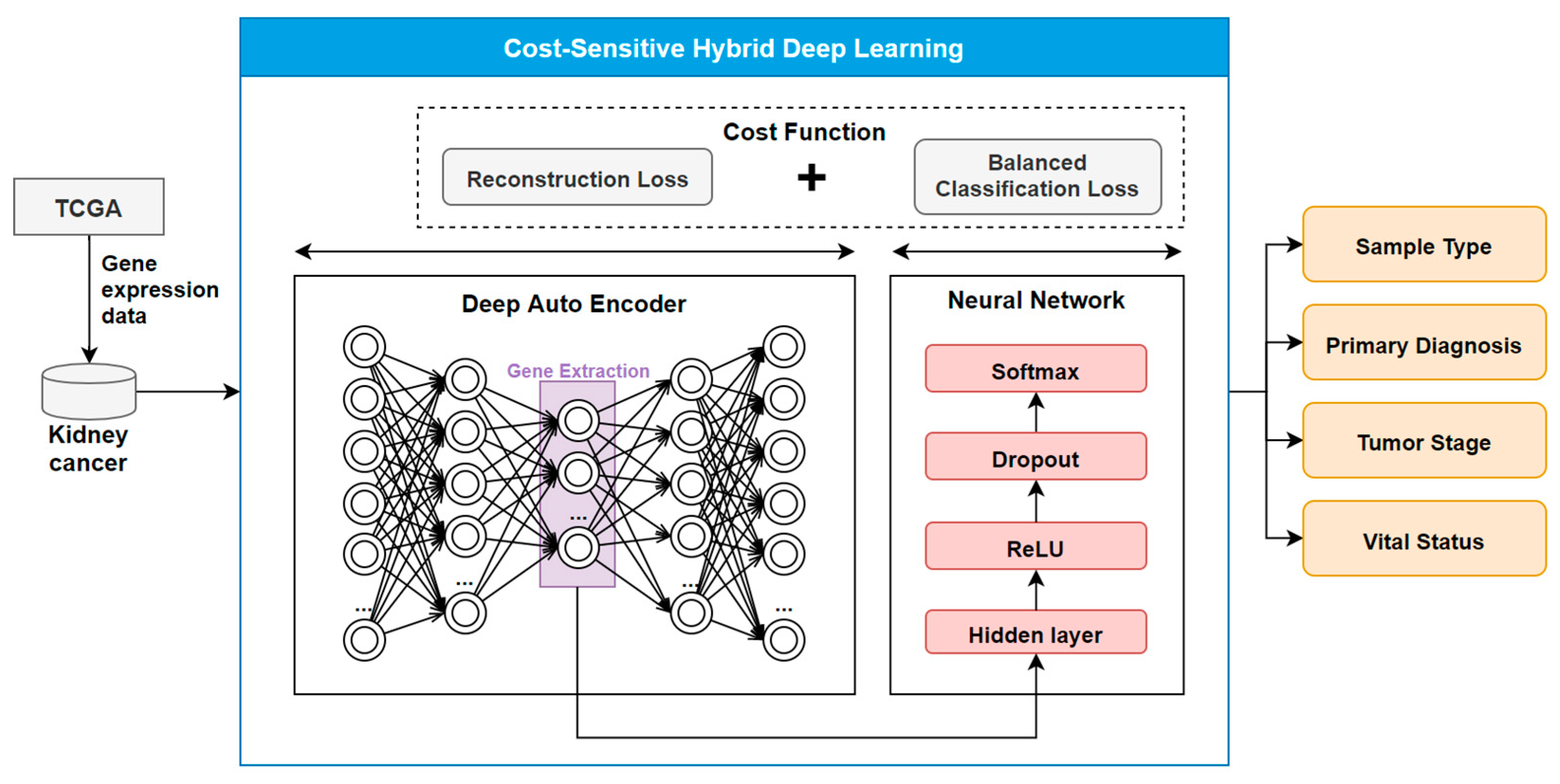
2.2. The COST-HDL Approach

In the experiments, the extracted target genes were subject to classification analysis, and the performance was evaluated. Figure 1 shows the proposed COST-HDL approach which input the gene expression data of kidney cancer from the TCGA portal and output four kinds of prognoses namely, sample type, primary diagnosis, tumor stage, and vital status. It consists of a hybrid of DAE and NN models. For the RNA sequencing data, the number of variables is significantly higher than the number of samples. Therefore, general classification analysis is prohibited by technical challenges in dealing with more than 60,000 variables: it is challenging to apply the data mining and machine learning algorithms to the raw dataset. Therefore, in this study, we used the 5-layer DAE model (the first 2 layers for encoding, the middle layer for gene extraction, and the last 2 layers for decoding) to extract significant genes and extract deep features from gene biomarkers as a result. The extracted deep features were input to the NN classification method (hidden layer + dropout [25] + Rectified Linear Unit (ReLU) [26] + softmax [27]).

The DAE model employed the mean squared error (MSE) as a reconstruction loss during the training, while the NN model used the focal loss [28] as a balanced classification loss. Focal loss is the reshaping of cross-entropy loss such that it down-weights the loss assigned to well-classified examples. The novel focal loss focuses on training on a sparse set of hard examples and prevents the vast number of easy negatives from overwhelming the detector during training. The proposed COST-HDL approach uses the sum of the reconstruction loss and balanced classification loss as a cost function.

The experimental hardware platform was the Intel Xeon E3 (32G memory, GTX 1080 Ti). We used Ubuntu 18.04 as the computational environment, and Python 3.7 was used for data collection and analysis. Python 3.7 Library uses Scikit-Learn [29] and Pytorch [30]. The following paragraphs describe the DAE model for extracting deep features from gene biomarkers and the NN model for constructing prognosis prediction models in detail.

2.2.1. Extracting Deep Features from Gene Biomarkers

We utilized the training dataset to extract gene expression data by using the DAE non-linear feature transformation method, and we compared it with Principal Component Analysis (PCA) [31] linear feature transformation and the Least Absolute Shrinkage and Selection Operator (LASSO) [32] feature selection methods. PCA explains correlated multivariate data in a fewer number of linearly uncorrelated variables which are a linear combination of the original variable. Due to the linearity constraints, we developed a DAE with non-linear activation functions which give more accuracy in the reconstruction of data. However, the feature selection methods such as LASSO select the best features or a subset of the original feature set and do not alter the original representation of data [33]. Thus, they may lose some important information during a selection process when extracting a complex structure of cancer data.

We developed the DAE model using Pytorch to extract deep features from gene biomarkers. The architecture of the DAE model consists of encoder and decoder parts. The encoder part comprised one input layer, and three fully connected encoding hidden layers with 1000, 500, and 100 nodes, respectively. The last layer of the hidden layers was chosen to be the deep feature to extract the gene biomarkers. The decoder part comprised two fully connected decoding hidden layers with 500 and 1000 nodes, respectively. The last layer of the hidden layer was chosen to be the output layer (reconstructed input). These are used to transpose the encoding layer weights. The procedure can be formulated as below:

$$\begin{gathered} hidden\_encod{e}_1=ReLU\left(W_1\times input+b_1\right) \\ hidden\_encod{e}_2=ReLU\left(W_2\times hidden\_encod{e}_1+b_2\right) \\ hidden\_encod{e}_3=W_3\times hidden\_encod{e}_2+b_3 \\ hidden\_decod{e}_1=ReLU\left({W_2}^{\prime }\times hidden\_encod{e}_3+{b_2}^{\prime }\right) \\ reconstructed\_input=Tanh\left({W_1}^{\prime }\times hidden\_encod{e}_1+{b_1}^{\prime }\right) \end{gathered}$$

(1)

where $W_1$, $W_2$, and $W_3$ are the weight metrics between the layers with the size of N$\times$1000, 1000$\times$500, and 500$\times$100, respectively; N is the size of input or number of samples; $b_1, b_2$, and $b_3$ are the biases for each node; and $ReLU$ and $Tanh$ are non-linear activation functions. The terms with superscripts refer to the transpose metrics. The $hidden\_encod{e}_3$ layer was chosen to be the activity values of the deep features in this model. The DAE has a loss function to handle the data reconstruction error which can measure the error between the original data and the reconstructed data, and it employed the MSE as its loss function.

2.2.2. Constructing Prognose Prediction Models

For the prognose prediction models, we constructed a feedforward neural network, which contained one input layer, one hidden layer with 100 nodes, and one output layer. The deep features of the $hidden\_encod{e}_3$ in the DAE model were used as the input of the NN model. This procedure can be formulated as below:

$$\begin{gathered} hidde{n}_{layer}=ReLU\left(W_4\times hidde{n}_{encode}{}_3+b_4\right) \\ output=softmax\left(W_5\times hidden\_layer+b_5\right) \end{gathered}$$

(2)

where $W_4$ and $W_5$ are the weight metrics between the layers with the size of 100$\times$100 and 100 $\times$ C, respectively; C is the size of output or number of class types; $b_4$ and $b_5$ are the biases for each node; and $ReLU$ and $softmax$ are non-linear activation functions. The $softmax$ activation function computes softmax cross entropy between logits and labels, and the sum of its outputs to 1 makes an efficient probability analysis. A dropout layer was added after the $hidden\_layer$, which randomly set 20% of the output of that layer to 0. The NN has a loss function to handle classification error which can measure the error between the true class and prediction class and also addresses the class imbalance. The NN model employed the focal loss as its loss function. The focal loss addresses the class balance problem by reshaping the standard cross-entropy loss such that it down-weighs the loss assigned to well-classified examples.

2.2.3. Training the Models

The cost function $L$ was used to measure the difference between the input and the output:

$$\begin{gathered} L_{DAE}\left(input, reconstructe{d}_{input}\right)=MSE loss \\ {L}_{NN}\left(hidden\_encod{e}_3, output\right)=focal loss \\ L\left(input, output\right)=L_{DAE}+L_{NN} \end{gathered}$$

(3)

For the optimization, we selected Adam optimizer [34], which has several arguments to be set freely, as the strategy to update the weights and bias so that the minima could be found. After running different trials, the learning rate was finally set to 0.00001, and the batch size and epoch were set to 128 and 2000, respectively. The models were finally trained under the parameters mentioned above. We chose the checkpoint model which shows the lowest error on the training set. The activity values and weight metrics related to deep features were readouts.

3. Results

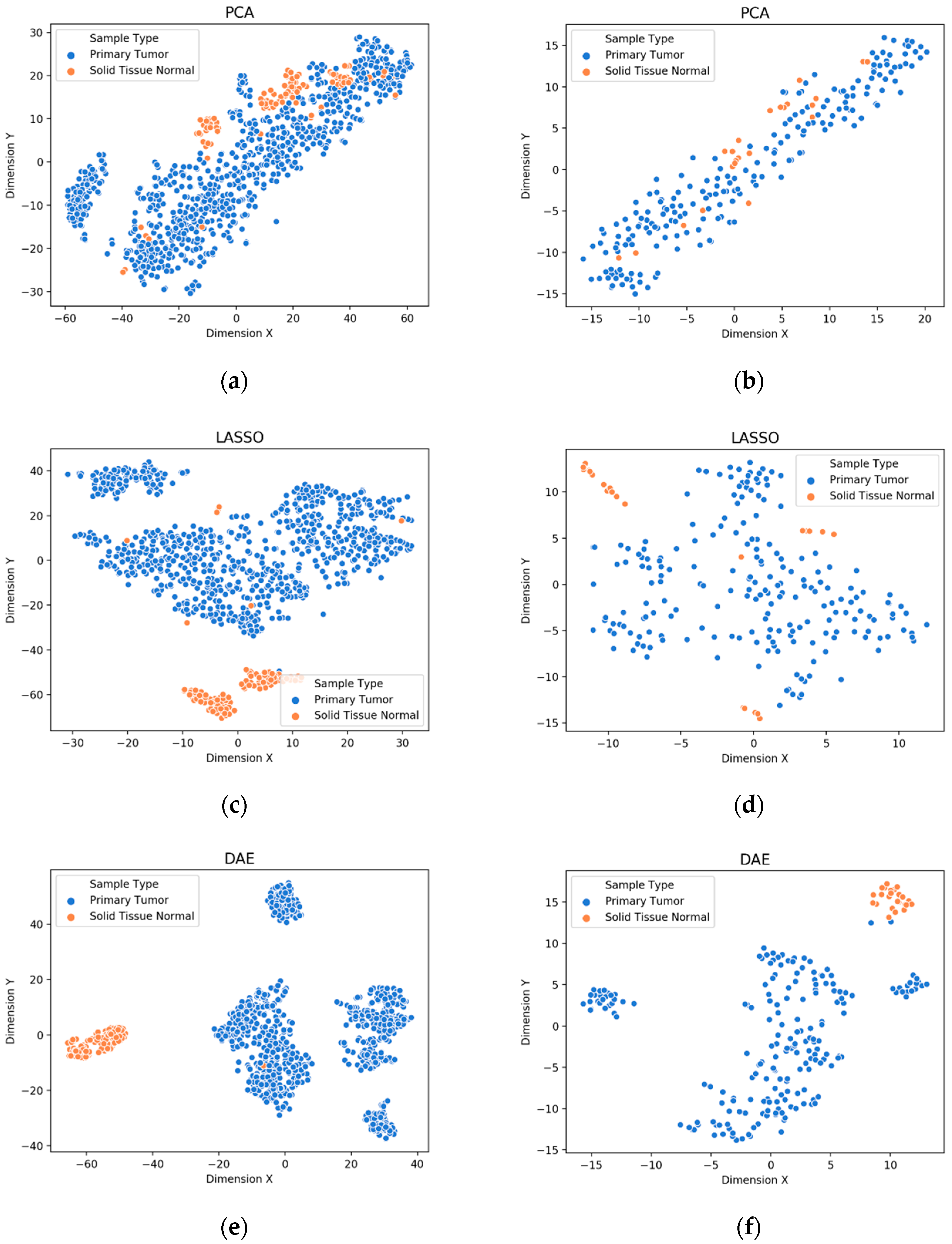
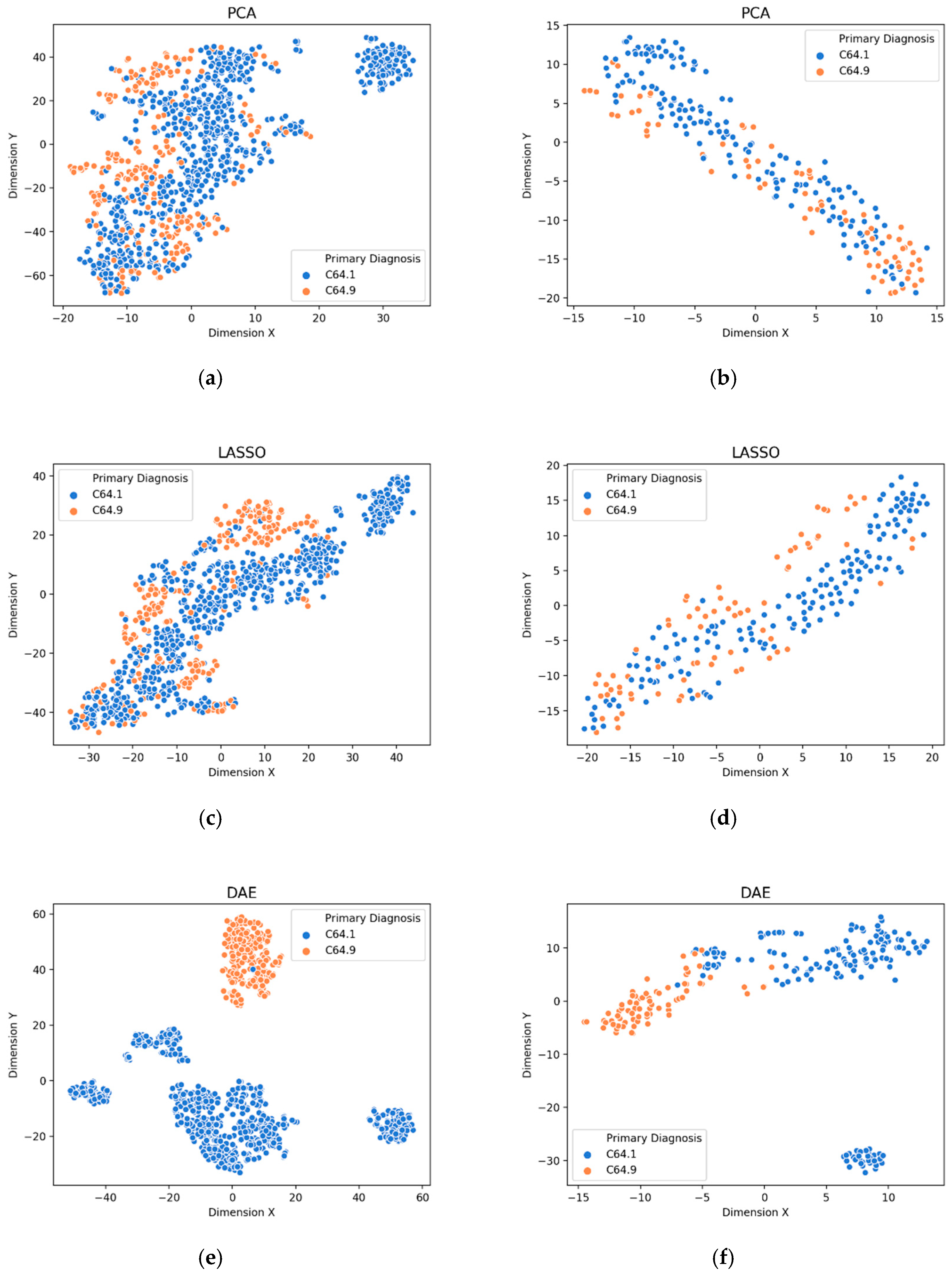
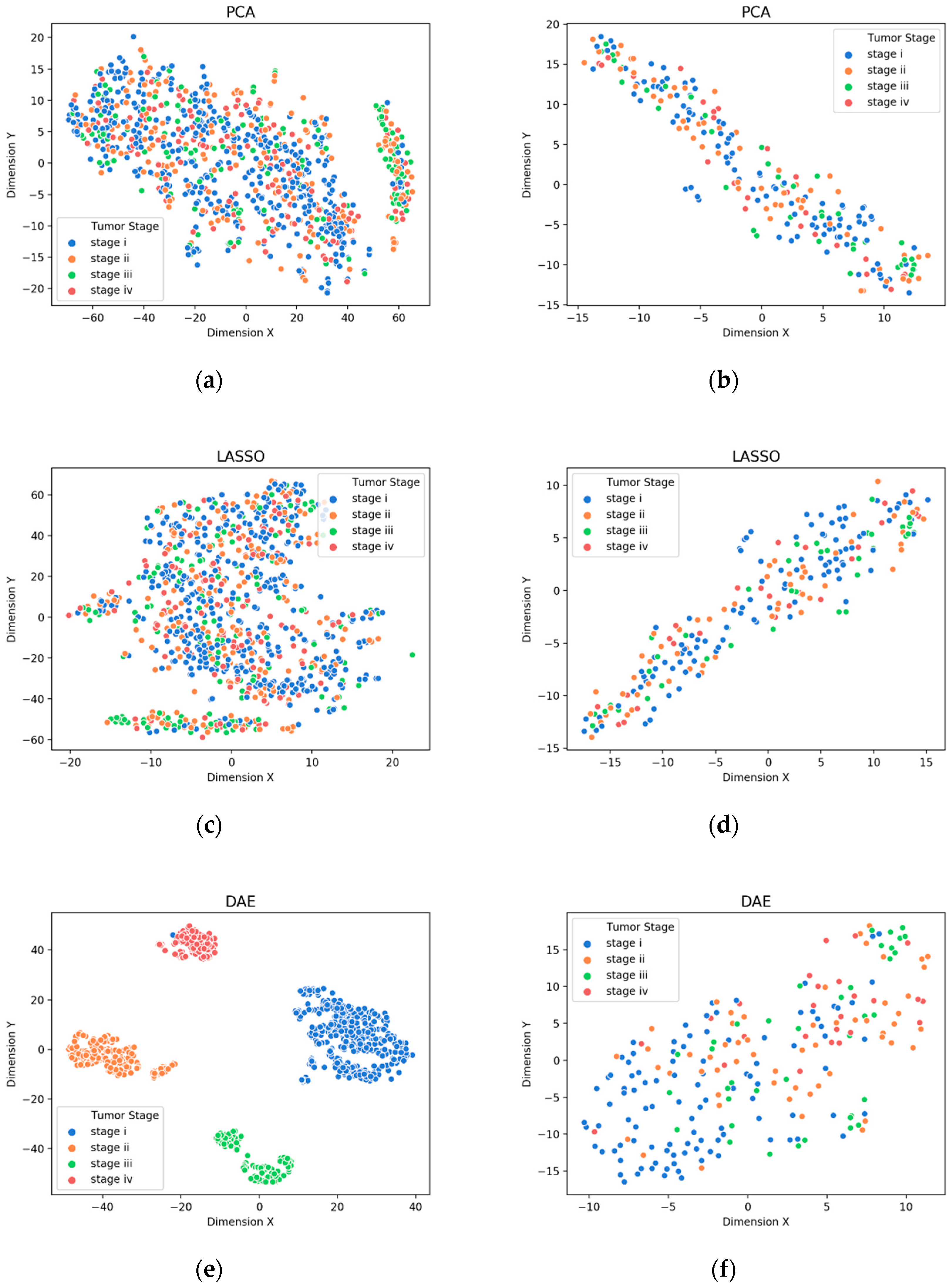
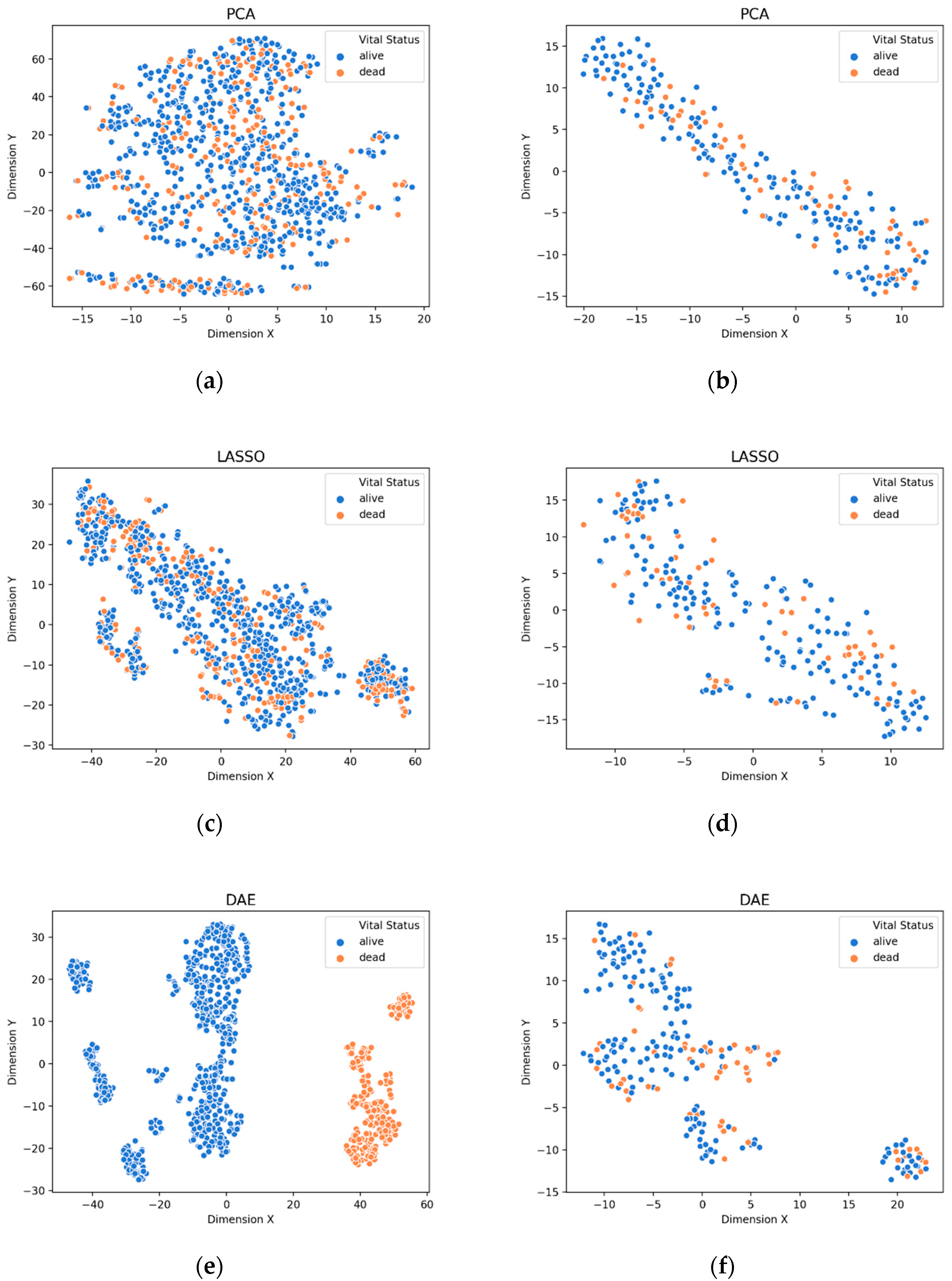
3.1. Visualization of Feature Extraction

The training set was utilized to analyze and extract deep features from gene biomarkers by the DAE model. We compared it with the PCA dimension reduction and LASSO feature selection methods. We extracted 100 features for each classification task for further analysis by the DAE model as shown in

Table 2. The extracted the number of deep features from gene biomarkers by the DAE model.

Prognosis	# Features
Sample Type	100
Primary Diagnosis	100
Tumor Stage	100
Vital Status	100

. For a fair comparison, we also extracted 100 features for each classification task by the PCA method as shown in

Table 3. The extracted number of features from gene biomarkers by PCA method.

Prognosis	# Features
Sample Type	100
Primary Diagnosis	100
Tumor Stage	100
Vital Status	100

. Different numbers of gene biomarkers were selected by the LASSO method as shown in

Table 4. The selected number of gene biomarkers by LASSO method.

Prognosis	# Gene Biomarkers
Sample Type	22
Primary Diagnosis	77
Tumor Stage	263
Vital Status	139

. The testing set was utilized to evaluate the feature extraction from gene biomarkers. We developed the PCA and LASSO methods using Scikit-Learn and developed the DAE model using Pytorch.

For the visualization of the deep features extracted by DAE, the features extracted by PCA, and the features selected by LASSO, we used t-Distributed Stochastic Neighbor Embedding (TSNE) [35]. TSNE is a widely used non-linear dimensionality reduction technique for visualizing high-dimensional data with clear and perfect separation on the two- (or three-) dimensional plane.

We used the two-dimensional plane for the following visualizations of extracted features as shown in Figure 2, Figure 3, Figure 4 and Figure 5 for each prognosis.

The visualization of the extracted features from the gene biomarkers for the prognosis such as sample type, primary diagnosis, tumor stage, and vital status are shown in Figure 2, Figure 3, Figure 4 and Figure 5, respectively. It can be seen that the deep features extracted by the DAE model were distinguished better than the features extracted by the PCA method and the features selected by the LASSO method on both the training and testing sets. Further, other prognoses are identified by the DAE method.

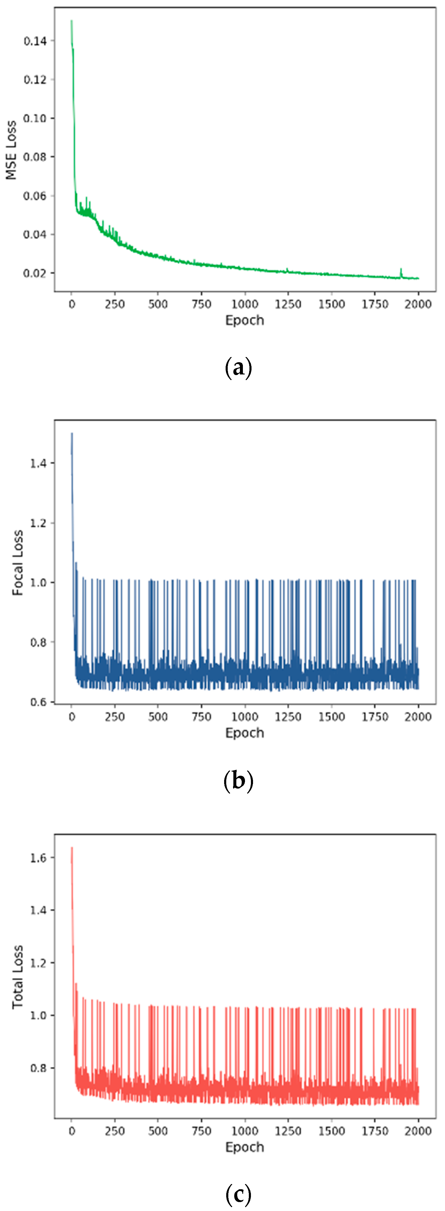
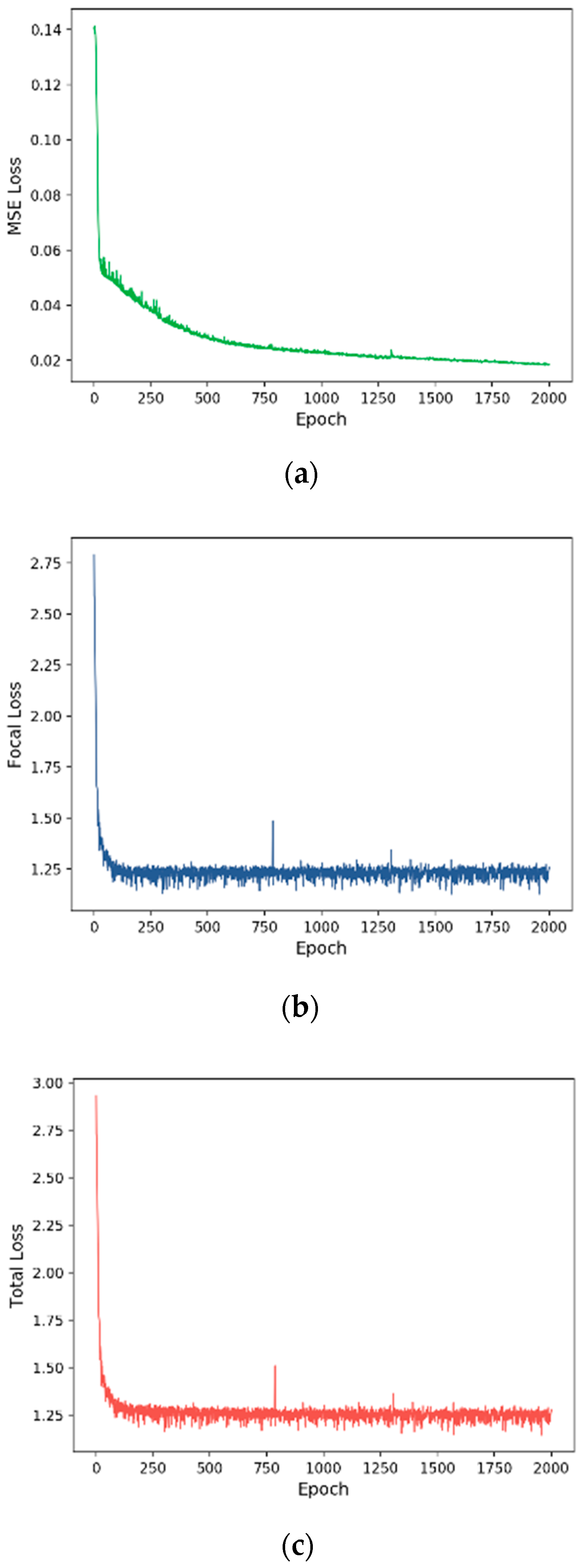
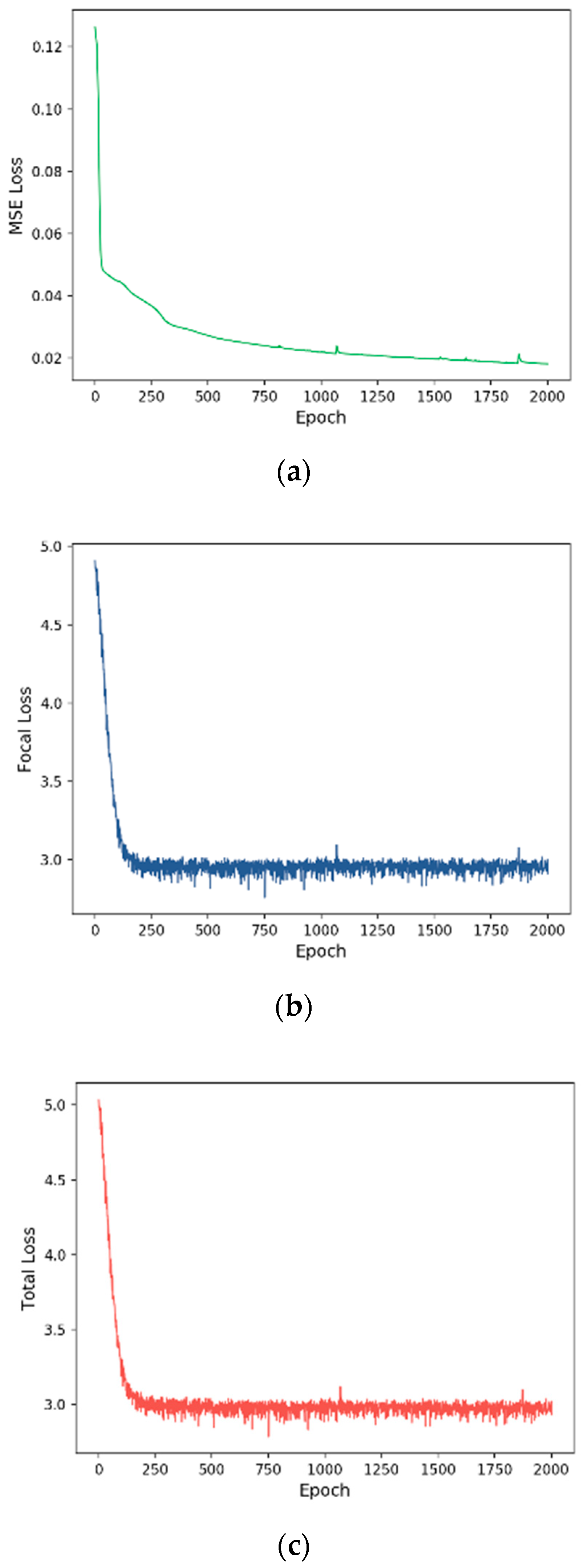
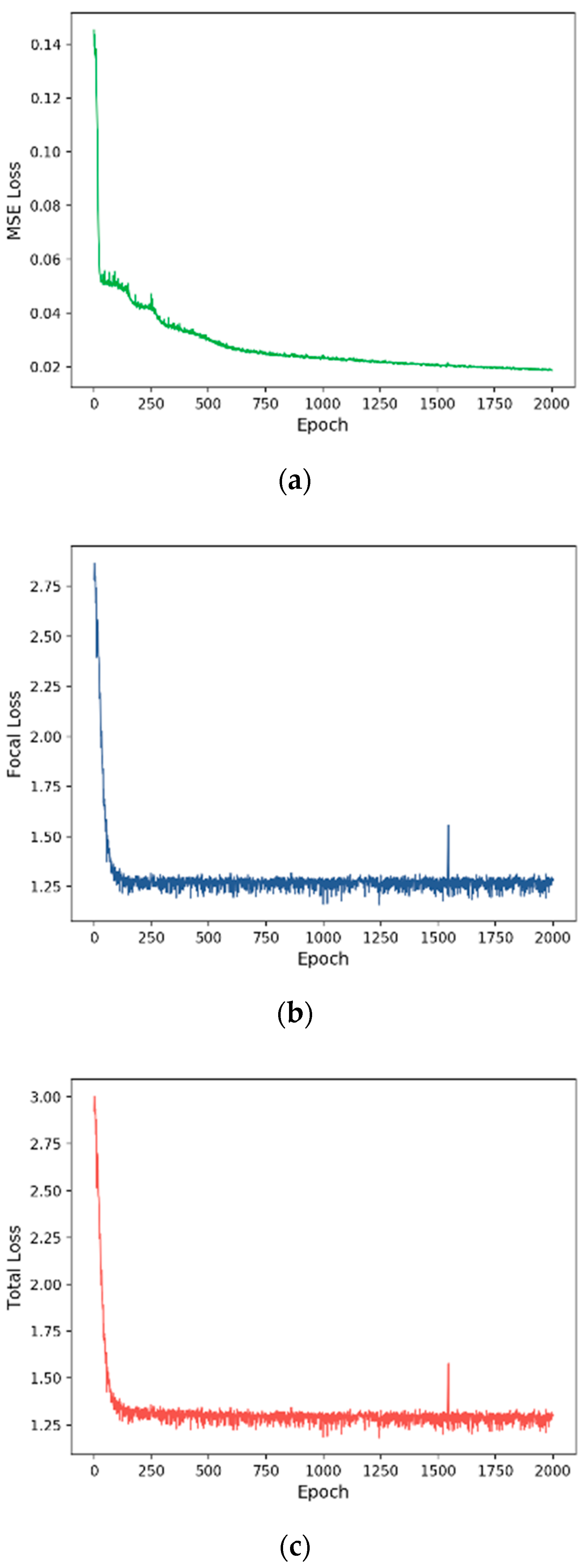
3.2. Training Process

We trained our COST-HDL approach with 2000 epochs. Each loss (MSE, Focal, and Total) during the training is shown in Figure 6, Figure 7, Figure 8 and Figure 9 for each prognosis. The MSE loss continuously decreased in all experiments for each diagnosis. In the multi-class case, tumor stage prognosis, it decreased more strictly. The focal loss decreased, but it was more sensitive during the training for each prognosis. In the binary class case, sample type prognosis, it was most sensitive and between the values 0.6 and 1. This was because the model was already satisfied with 100% of performance results.

3.3. Evaluation of Prognose Prediction Models

To evaluate our COST-HDL approach, four indices namely, accuracy, precision, recall, and f1-score were employed the classification performance, and they are defined as follows.

$$\begin{gathered} Accuracy=\frac{TP+TN}{TP+TN+FP+FN} \\ Precision=\frac{TP}{TP+FP} \\ Recall=\frac{TP}{TP+FN} \\ F1-score=\frac{2\times Precision\times Recall}{Precision+Recall} \end{gathered}$$

(4)

where $TP, TN, FP,$ and $FN$ are the number of true positives, true negatives, false positives, and false negatives, respectively. A true positive is an outcome where the model correctly predicts the positive class. Similarly, a true negative is an outcome where the model correctly predicts the negative class. A false positive is an outcome where the model incorrectly predicts the positive class, and a false negative is an outcome where the model incorrectly predicts the negative class. In

Table 5. Effect of loss function of the COST-HDL approach. The best results are shown in bold.

Prognosis	Loss	Accuracy	Precision	Recall	F1-Score
Sample Type	MSE	89.13	44.57	50.00	47.13
	Focal	99.57	99.76	98.00	98.86
	Total	100.00	100.00	100.00	100.00
Primary Diagnosis	MSE	62.93	43.86	47.89	42.63
	Focal	96.55	97.13	95.01	95.97
	Total	96.98	97.43	95.68	96.49
Tumor Stage	MSE	12.05	7.92	26.32	7.31
	Focal	54.46	45.15	45.05	43.76
	Total	56.70	49.41	46.14	46.68
Vital Status	MSE	73.71	36.85	50.00	42.43
	Focal	76.29	69.00	67.05	67.83
	Total	76.72	69.78	68.92	69.32

, we compared the models with different loss functions (only MSE loss, only focal loss, and total loss). It can be seen that the models with total loss show better performances than the other single loss models, and the models with only MSE loss show the worst results.

For the prediction of sample type prognosis, our COST-HDL approach with total loss achieved the highest results: 100% accuracy, 100% precision, 100% recall, and 100% f1-score. It improved the model with only focal loss by 0.43% of accuracy, 0.24% of precision, 2% of recall, and 1.14% of f1-score.

For the prediction of primary diagnosis prognosis, our COST-HDL approach with total loss achieved the highest results: 96.98% accuracy, 97.43% precision, 95.68% recall, and 96.49% f1-score. It improved the model with only focal loss by 0.43% of accuracy, 0.3% of precision, 0.67% of recall, and 0.52% of f1-score.

For the prediction of tumor stage prognosis, our COST-HDL approach with total loss achieved the highest results: 56.70% accuracy, 49.41% precision, 46.14% recall, and 46.68% f1-score. It improved the model with only focal loss by 2.24% of accuracy, 4.26% of precision, 1.09% of recall, and 2.92% of f1-score.

For the prediction of vital status prognosis, our COST-HDL approach with total loss achieved the highest results: 76.72% accuracy, 69.78% precision, 68.92% recall, and 69.32% f1-score. It improved the model with only focal loss by 0.43% of accuracy, 0.78% of precision, 1.87% of recall, and 1.49% of f1-score.

We verified whether our COST-HDL approach performs better than general traditional machine learning classifiers, such as K-Nearest Neighbors (KNN) [36], Linear Support Vector Machine (Linear SVM) [37], Kernel Support Vector Machine (Kernel SVM) [38], Random Forest (RF) [39], and Neural Network (NN) [40]. The traditional machine learning classifiers are followed by feature extraction methods such as PCA dimension reduction and LASSO feature selection. To solve the data imbalance problem, they usually employ sampling methods such as the Synthetic Minority Over-sampling Technique (SMOTE) [41], which is an over-sampling method.

Hence, in this paper, we compared our COST-HDL approach with a total loss to the traditional combination of methods: feature extraction → sampling → classifier, as shown in

Table 6. Evaluation of prediction models for sample type. The best results are shown in bold.

Classifier	Feature	Sampling	Accuracy	Precision	Recall	F1-Score
KNN	PCA	No	98.70	99.28	94.00	96.45
		Yes	96.52	88.46	96.29	91.87
	LASSO	No	98.70	97.43	95.76	96.57
		Yes	99.57	98.08	99.76	98.90
Linear SVM	PCA	No	97.39	90.32	98.54	93.90
		Yes	97.83	91.67	98.78	94.84
	LASSO	No	99.13	96.30	99.51	97.83
		Yes	98.70	94.64	99.27	96.80
Kernel SVM	PCA	No	89.13	44.57	50.00	47.13
		Yes	89.13	44.57	50.00	47.13
	LASSO	No	89.13	44.57	50.00	47.13
		Yes	89.13	44.57	50.00	47.13
RF	PCA	No	95.65	97.67	80.00	86.31
		Yes	97.39	98.58	88.00	92.46
	LASSO	No	99.13	99.52	96.00	97.67
		Yes	100.00	100.00	100.00	100.00
NN	PCA	No	98.26	95.51	95.51	95.51
		Yes	98.26	95.51	95.51	95.51
	LASSO	No	99.13	96.30	99.51	97.83
		Yes	99.57	98.08	99.76	98.90
COST-HDL			100.00	100.00	100.00	100.00

,

Table 7. Evaluation of prediction models for primary diagnosis. The best results are shown in bold.

Classifier	Feature	Sampling	Accuracy	Precision	Recall	F1-Score
KNN	PCA	No	87.07	87.01	82.79	84.40
		Yes	84.91	82.82	82.59	82.70
	LASSO	No	88.79	90.21	84.06	86.24
		Yes	89.66	90.35	85.74	87.52
Linear SVM	PCA	No	88.79	86.67	89.28	87.67
		Yes	92.67	91.32	92.15	91.71
	LASSO	No	94.40	94.03	93.07	93.53
		Yes	95.69	95.37	94.73	95.04
Kernel SVM	PCA	No	67.67	33.84	50.00	40.36
		Yes	67.67	33.84	50.00	40.36
	LASSO	No	67.67	33.84	50.00	40.36
		Yes	67.67	33.84	50.00	40.36
RF	PCA	No	90.52	93.85	85.33	88.13
		Yes	94.83	96.45	92.00	93.81
	LASSO	No	92.24	94.24	88.35	90.56
		Yes	94.40	94.75	92.38	93.43
NN	PCA	No	89.22	88.50	86.47	87.36
		Yes	88.36	87.76	85.13	86.25
	LASSO	No	92.24	91.65	90.44	91.01
		Yes	92.24	92.73	89.39	90.79
COST-HDL			96.98	97.43	95.68	96.49

,

Table 8. Evaluation of prediction models for tumor stage. The best results are shown in bold.

Classifier	Feature	Sampling	Accuracy	Precision	Recall	F1-Score
KNN	PCA	No	47.77	38.39	33.62	32.66
		Yes	41.07	33.60	33.14	32.91
	LASSO	No	45.09	32.25	30.07	28.96
		Yes	40.18	34.27	35.24	34.13
Linear SVM	PCA	No	29.91	27.61	27.15	24.73
		Yes	26.34	39.21	32.28	25.64
	LASSO	No	40.62	37.24	40.47	34.28
		Yes	50.00	43.01	38.21	36.61
Kernel SVM	PCA	No	46.43	11.61	25.00	15.85
		Yes	46.43	11.61	25.00	15.85
	LASSO	No	46.43	11.61	25.00	15.85
		Yes	46.43	11.61	25.00	15.85
RF	PCA	No	51.34	51.20	33.43	32.12
		Yes	54.46	48.20	44.30	44.77
	LASSO	No	55.36	55.87	39.11	39.07
		Yes	53.12	45.43	45.56	44.47
NN	PCA	No	46.88	38.89	38.65	38.75
		Yes	47.32	40.36	40.81	40.45
	LASSO	No	41.52	35.67	35.33	35.23
		Yes	45.54	38.23	37.98	38.01
COST-HDL			56.70	49.41	46.14	46.68

and

Table 9. Evaluation of prediction models for vital status. The best results are shown in bold.

Classifier	Feature	Sampling	Accuracy	Precision	Recall	F1-Score
KNN	PCA	No	70.69	57.64	54.81	54.64
		Yes	65.09	54.75	54.70	54.72
	LASSO	No	66.38	51.15	50.83	50.29
		Yes	65.52	55.10	54.99	55.04
Linear SVM	PCA	No	64.66	57.54	58.62	57.71
		Yes	58.19	52.62	53.18	52.05
	LASSO	No	73.71	63.48	57.38	57.60
		Yes	72.84	62.39	58.38	58.94
Kernel SVM	PCA	No	73.71	36.85	50.00	42.43
		Yes	73.71	36.85	50.00	42.43
	LASSO	No	73.71	36.85	50.00	42.43
		Yes	73.71	36.85	50.00	42.43
RF	PCA	No	73.71	62.50	53.16	50.42
		Yes	70.26	58.66	56.62	56.95
	LASSO	No	75.00	66.56	58.79	59.33
		Yes	73.28	65.73	66.05	65.88
NN	PCA	No	62.07	53.38	53.71	53.41
		Yes	58.62	53.68	54.53	53.04
	LASSO	No	61.21	54.86	55.76	54.69
		Yes	58.19	54.23	55.29	53.31
COST-HDL			76.72	69.78	68.92	69.32

for each prognosis.

For the sample type prognosis, the RF classifier with LASSO feature selection and SMOTE sampling achieved 100% accuracy, 100% precision, 100% recall, and 100% f1-score. The second-best results were 99.57% accuracy, 98.08% precision, 99.76% recall, and 98.90% f1-score achieved by the KNN and NN with LASSO feature selection and SMOTE sampling. The worst results were achieved by Kernel SVM.

For the primary diagnosis prognosis, the second-best results were 95.69% accuracy, 95.37% precision, 94.73% recall, and 95.04% f1-score achieved by the Linear SVM with LASSO feature selection and SMOTE sampling. The worst results were achieved by Kernel SVM.

For the tumor stage prognosis, the second-best results were 55.36% accuracy, 55.87% precision, 39.11% recall, and 39.07% f1-score achieved by the RF with LASSO feature selection and without SMOTE sampling. The worst results were achieved by the Linear SVM with PCA and SMOTE sampling.

For the vital status prognosis, the second-best results were 75.00% accuracy, 66.56% precision, 58.79% recall, and 59.33% f1-score achieved by the RF with LASSO feature selection and without SMOTE sampling. The worst results were achieved by the Linear SVM with PCA and SMOTE sampling.

4. Discussion and Conclusions

In this study, we showed that unsupervised non-linear DAE is an effective model to extract meaningful deep features of gene expression data from patients with kidney cancer. These features were significantly associated with the kidney cancer prognosis such as sample type, primary diagnosis, tumor stage, and vital status representing the state of patients. We also showed that the end-to-end hybrid deep learning architecture is more effective than the traditional machine learning analysis flow: feature extraction, sampling, classification.

We compared the proposed COST-HDL approach with other traditional approaches, and it achieved better results for all prognosis on gene expression data. The deep features extracted by the DAE model were distinguished better than the features extracted by the PCA method and the features selected by the LASSO method on both the training and testing sets. Further, another class label was identified by the DAE method. The results obtained can be applied to extract deep features from gene biomarkers for prognosis prediction of kidney cancer from various causes and; hence, it is useful for preventing kidney cancer and early diagnosis.

This study can be improved in three ways. The first is to develop unsupervised deep symmetric autoencoder methods such as stacking more layers, denoising, or variational functions. The second is to modify loss function which can also handle the imbalance problem, reconstruction, and classification error. The third is to improve the classifier instead of using the only neural network, and add more layers or replace existing ones by other methods such as random forest, support vector machine, k nearest neighbor, etc. Although the experimental results show that the proposed hybrid approach has the potential to improve the prognosis prediction of kidney cancer, the identification of significant biomarkers and interpretability of the deep learning model is limited in our research. In the healthcare field, interpretability is one of the primary problems with deep learning, known as black-box. The proposed approach can be extended by addressing the problem of interpretability and the human-readability of deep learning models. We will explore these ideas in future analysis.

References

1. Xiong, H.Y.; Alipanahi, B.; Lee, L.J.; Bretschneider, H.; Merico, D.; Yuen, R.K.C.; Hua, Y.; Gueroussov, S.; Najafabadi, H.S.; Hughes, T.R.; et al. The human splicing code reveals new insights into the genetic determinants of disease. Science 2015, 347, 1254806. [Google Scholar] [CrossRef] [PubMed] [Green Version]
2. Korean National Cancer Center. Available online: https://www.ncc.re.kr (accessed on 23 November 2019).
3. Câmara, N.O.S.; Iseki, K.; Kramer, H.; Liu, Z.H.; Sharma, K. Kidney disease and obesity: Epidemiology, mechanisms and treatment. Nat. Rev. Nephrol. 2017, 13, 181–190. [Google Scholar] [CrossRef] [PubMed]
4. D’Angelo, G.; Pilla, R.; Tascini, C.; Rampone, S. A proposal for distinguishing between bacterial and viral meningitis using genetic programming and decision trees. Soft Comput. 2019, 23, 11775–11791. [Google Scholar] [CrossRef]
5. Bejnordi, B.E.; Veta, M.; Van Diest, P.J.; Van Ginneken, B.; Karssemeijer, N.; Litjens, G.; Van Der Laak, J.A.W.M.; Hermsen, M.; Manson, Q.F.; Balkenhol, M.; et al. Diagnostic assessment of deep learning algorithms for detection of lymph node metastases in women with breast cancer. JAMA 2017, 318, 2199–2210. [Google Scholar] [CrossRef] [PubMed]
6. Amgad, M.; Elfandy, H.; Hussein, H.; Atteya, L.A.; Elsebaie, M.A.; Abo Elnasr, L.S.; Sakr, R.A.; Salem, H.S.; Ismail, A.F.; Saad, A.M.; et al. Structured crowdsourcing enables convolutional segmentation of histology images. Bioinformatics 2019, 35, 3461–3467. [Google Scholar] [CrossRef] [PubMed] [Green Version]
7. Kim, B.J.; Kim, S.H. Prediction of inherited genomic susceptibility to 20 common cancer types by a supervised machine-learning method. Proc. Natl. Acad. Sci. USA 2018, 115, 1322–1327. [Google Scholar] [CrossRef] [Green Version]
8. Chen, Y.; Li, Y.; Narayan, R.; Subramanian, A.; Xie, X. Gene expression inference with deep learning. Bioinformatics 2016, 32, 1832–1839. [Google Scholar] [CrossRef] [Green Version]
9. Ferroni, P.; Zanzotto, F.M.; Riondino, S.; Scarpato, N.; Guadagni, F.; Roselli, M. Breast cancer prognosis using a machine learning approach. Cancers 2019, 11, 328. [Google Scholar] [CrossRef] [Green Version]
10. Chen, M.; Hao, Y.; Hwang, K.; Wang, L.; Wang, L. Disease prediction by machine learning over big data from healthcare communities. IEEE Access 2017, 5, 8869–8879. [Google Scholar] [CrossRef]
11. Muhamed Ali, A.; Zhuang, H.; Ibrahim, A.; Rehman, O.; Huang, M.; Wu, A. A machine learning approach for the classification of kidney cancer subtypes using miRNA genome data. Appl. Sci. 2018, 8, 2422. [Google Scholar] [CrossRef] [Green Version]
12. Aljouie, A.; Patel, N.; Roshan, U. Cross-validation and cross-study validation of kidney cancer with machine learning and whole exome sequences from the National Cancer Institute. In Proceedings of the 2018 IEEE Conference on Computational Intelligence in Bioinformatics and Computational Biology (CIBCB), St. Louis, MO, USA, 30 May–2 June 2018; pp. 1–6. [Google Scholar]
13. Ing, N.; Huang, F.; Conley, A.; You, S.; Ma, Z.; Klimov, S.; Ohe, C.; Yuan, X.; Amin, M.B.; Figlin, R.; et al. A novel machine learning approach reveals latent vascular phenotypes predictive of renal cancer outcome. Sci. Rep. 2017, 7, 13190. [Google Scholar] [CrossRef] [Green Version]
14. Kourou, K.; Exarchos, T.P.; Exarchos, K.P.; Karamouzis, M.V.; Fotiadis, D.I. Machine learning applications in cancer prognosis and prediction. Comput. Struct. Biotechnol. J. 2015, 13, 8–17. [Google Scholar] [CrossRef] [PubMed] [Green Version]
15. Wolf, F.A.; Angerer, P.; Theis, F.J. SCANPY: Large-scale single-cell gene expression data analysis. Genome Biol. 2018, 19, 15. [Google Scholar] [CrossRef] [Green Version]
16. Libbrecht, M.; Noble, W. Machine learning applications in genetics and genomics. Nat. Rev. Genet. 2015, 16, 321–332. [Google Scholar] [CrossRef] [Green Version]
17. Zeng, W.Z.D.; Glicksberg, B.S.; Li, Y.; Chen, B. Selecting precise reference normal tissue samples for cancer research using a deep learning approach. BMC Med. Genomics 2019, 12, 21. [Google Scholar] [CrossRef] [Green Version]
18. Danaee, P.; Ghaeini, R.; Hendrix, D.A. A deep learning approach for cancer detection and relevant gene identification. Pac. Symp. Biocomput. 2017, 2017, 219–229. [Google Scholar]
19. Kim, B.H.; Yu, K.; Lee, P.C. Cancer classification of single-cell gene expression data by neural network. Bioinformatics 2019. [Google Scholar] [CrossRef]
20. Xie, R.; Wen, J.; Quitadamo, A.; Cheng, J.; Shi, X. A deep auto-encoder model for gene expression prediction. BMC Genomics 2017, 18, 845. [Google Scholar] [CrossRef] [PubMed] [Green Version]
21. Gupta, A.; Wang, H.; Ganapathiraju, M. Learning structure in gene expression data using deep architectures, with an application to gene clustering. In Proceedings of the 2015 IEEE International Conference on Bioinformatics and Biomedicine (BIBM), Washington, DC, USA, 9–12 November 2015; pp. 1328–1335. [Google Scholar]
22. Genomic Data Commons Data Portal. Available online: https://portal.gdc.cancer.gov (accessed on 23 November 2019).
23. Wang, H.; Li, B.; Leng, C. Shrinkage tuning parameter selection with a diverging number of parameters. J. R. Stat. Soc. Ser. B Stat. Methodol. 2009, 71, 671–683. [Google Scholar] [CrossRef]
24. Mortazavi, A.; Williams, B.A.; McCue, K.; Schaeffer, L.; Wold, B. Mapping and quantifying mammalian transcriptomes by RNA-Seq. Nat. Methods 2008, 5, 621. [Google Scholar] [CrossRef]
25. Srivastava, N.; Hinton, G.; Krizhevsky, A.; Sutskever, I.; Salakhutdinov, R. Dropout: A simple way to prevent neural networks from overfitting. J. Mach. Learn. Res. 2014, 15, 1929–1958. [Google Scholar]
26. Nair, V.; Hinton, G.E. Rectified linear units improve restricted boltzmann machines. In Proceedings of the 27th International Conference on Machine Learning (ICML 2010), Haifa, Israel, 21–24 June 2010; pp. 807–814. [Google Scholar]
27. Grave, E.; Joulin, A.; Cissé, M.; Jégou, H. Efficient softmax approximation for GPUs. In Proceedings of the 34th International Conference on Machine Learning (ICML 2017), Sydney, Australia, 6–11 August 2017; Volume 70, pp. 1302–1310. [Google Scholar]
28. Lin, T.Y.; Goyal, P.; Girshick, R.; He, K.; Dollár, P. Focal loss for dense object detection. In Proceedings of the IEEE International Conference on Computer Vision, Venice, Italy, 22–29 October 2017; pp. 2980–2988. [Google Scholar]
29. Pedregosa, F.; Varoquaux, G.; Gramfort, A.; Michel, V.; Thirion, B.; Grisel, O.; Blondel, M.; Prettenhofer, P.; Weiss, R.; Dubourg, V.; et al. Scikit-learn: Machine learning in Python. J. Mach. Learn. Res. 2011, 12, 2825–2830. [Google Scholar]
30. PyTorch. Available online: https://pytorch.org (accessed on 23 November 2019).
31. Wold, S.; Esbensen, K.; Geladi, P. Principal component analysis. Chemom. Intell. Lab. Syst. 1987, 2, 37–52. [Google Scholar] [CrossRef]
32. Tibshirani, R. Regression shrinkage and selection via the lasso. J. R. Stat. Soc. Ser. B Methodol. 1996, 58, 267–288. [Google Scholar] [CrossRef]
33. Saeys, Y.; Inza, I.; Larrañaga, P. A review of feature selection techniques in bioinformatics. Bioinformatics 2007, 23, 2507–2517. [Google Scholar] [CrossRef] [Green Version]
34. Kingma, D.P.; Ba, J. Adam: A method for stochastic optimization. arXiv 2014, arXiv:1412.6980. [Google Scholar]
35. Maaten, L.V.D.; Hinton, G. Visualizing data using t-SNE. J. Mach. Learn. Res. 2008, 9, 2579–2605. [Google Scholar]
36. Goldberger, J.; Hinton, G.E.; Roweis, S.T.; Salakhutdinov, R.R. Neighbourhood components analysis. In Proceedings of the Advances in Neural Information Processing Systems, Vancouver, BC, Canada, 5–8 December 2005; pp. 513–520. [Google Scholar]
37. Tang, Y. Deep learning using linear support vector machines. arXiv 2013, arXiv:1306.0239. [Google Scholar]
38. Scholkopf, B.; Smola, A.J. Learning with Kernels: Support Vector Machines, Regularization, Optimization, and Beyond; MIT Press: Cambridge, MA, USA, 2001. [Google Scholar]
39. Liaw, A.; Wiener, M. Classification and regression by randomForest. R News 2002, 2, 18–22. [Google Scholar]
40. Dreiseitl, S.; Ohno-Machado, L. Logistic regression and artificial neural network classification models: A methodology review. J. Biomed. Inform. 2002, 35, 352–359. [Google Scholar] [CrossRef] [Green Version]
41. Chawla, N.V.; Bowyer, K.W.; Hall, L.O.; Kegelmeyer, W.P. SMOTE: Synthetic minority over-sampling technique. J. Artif. Intell. Res. 2002, 16, 321–357. [Google Scholar] [CrossRef]
Figure 1. Overview of COST-HDL approach. We used kidney cancer gene expression data from the TCGA portal. The Deep Auto Encoder (DAE) model is used to extract deep features from gene biomarkers as a lower-dimensional vector. The Neural Network (NN) is used to classify sample type, primary diagnosis, tumor stage, and vital status. We summed the reconstruction loss (DAE) and balanced classification loss (NN) in the cost function.
Symmetry 12 00154 g001
Figure 2. Visualization of extracted features from gene biomarkers for sample type prognosis: (a) train data extracted by PCA, (b) test data extracted by PCA, (c) train data extracted by LASSO, (d) test data extracted by LASSO, (e) train data extracted by DAE, (f) test data extracted by DAE.
Symmetry 12 00154 g002
Figure 3. Visualization of extracted features from gene biomarkers for primary diagnosis prognosis: (a) train data extracted by PCA, (b) test data extracted by PCA, (c) train data extracted by LASSO, (d) test data extracted by LASSO, (e) train data extracted by DAE, (f) test data extracted by DAE.
Symmetry 12 00154 g003
Figure 4. Visualization of extracted features from gene biomarkers for tumor stage prognosis: (a) train data extracted by PCA, (b) test data extracted by PCA, (c) train data extracted by LASSO, (d) test data extracted by LASSO, (e) train data extracted by DAE, (f) test data extracted by DAE.
Symmetry 12 00154 g004
Figure 5. Visualization of extracted features from gene biomarkers for vital status prognosis: (a) train data extracted by PCA, (b) test data extracted by PCA, (c) train data extracted by LASSO, (d) test data extracted by LASSO, (e) train data extracted by DAE, (f) test data extracted by DAE.
Symmetry 12 00154 g005
Figure 6. Training loss for sample type prognosis: (a) MSE loss, (b) focal loss, (c) total loss. The x axis indicates the number of epochs, and the y axis indicates the loss.
Symmetry 12 00154 g006
Figure 7. Training loss for primary diagnosis prognosis: (a) MSE loss, (b) focal loss, (c) total loss. The x axis indicates the number of epochs, and the y axis indicates the loss.
Symmetry 12 00154 g007
Figure 8. Training loss for tumor stage prognosis: (a) MSE loss, (b) focal loss, (c) total loss. The x axis indicates the number of epochs, and the y axis indicates loss.
Symmetry 12 00154 g008
Figure 9. Training loss for vital status prognosis: (a) MSE loss, (b) focal loss, (c) total loss. The x axis indicates the number of epochs, and the y axis indicates the loss.
Symmetry 12 00154 g009