Multidimensional Interpolation Decoupling Strategy for CD Basis Weight of Papermaking Process

Abstract

With a focus on the multivariable coupling characteristics in a cross-directional (CD) basis weight control system, we study the coupling characteristics of a CD control system and decoupling control, and we propose a novel multivariable interpolation decoupling control strategy and a real-time decomposition algorithm in this paper. Based on a model of the CD basis weight profile, a system non-square interaction matrix of high-dimensional data is analyzed by experimental studies and numerical simulation. Along the diagonal of the interaction matrix, the matrix block method is adopted to reduce the system dimension and convert it into a square system. A multivariable control system with high dimensionality is divided into several subsystems. For the high-dimensional Toeplitz symmetric subsystem with small-scale coupling characteristics, an interpolation decoupling algorithm is proposed. Then, a decoupling compensator with the structure of a symmetric Toeplitz matrix was obtained. Compared with the conventional diagonal decoupling matrix, the branch number of the new decoupling network is reduced from 2408 to 186, which realizes the fast decoupling of multivariable systems. The results were even better when we used a double size interaction matrix obtained by interpolation between actual values. By designing the diagonalized controller for the new decoupled system, a decouped CD control system for corrugated paper with a basis weight of 133 g/m² was implemented in an actual project in a paper mill.

1. Introduction

Paper-making is by far the most complex and complicated of all the pulp and paper processes. An important quality characteristic in the production of paper sheets is the range of functions in the basis weight, which should be kept as small as possible. The quality of the manufactured paper is assessed in two dimensions: one is the maintenance of the average sheet property profile along the paper sheet as it moves while it is being manufactured, which is referred to as machine directional (MD) control, and the other is the maintenance of the sheet profile across the width of the paper machine, which is referred to as cross-directional (CD) control. In the process of modern high-speed paper machines, it is necessary to monitor and control the performance of paper continuously to ensure that the quality of paper meets the requirements of MD and CD [1]. The CD basis weight profile is a very important quality index of paper in the papermaking process. Control of the CD basis weight on paper machines has long been known as an especially difficult problem. This is due to several difficulties including the high dimensionality of the cross-directional system, the high lateral space interaction between actuators, the uncertainty of the model, and the limited control authority of the actuator [2].

The primary reason for the difficulty of CD control is the complexity of the profile response to a slice adjustment [3]. The modern hydraulic headbox is equipped with dilution water supply equipment for basis weight profile control. The adjustment of the CD profile by dilution water is superior to the traditional slice adjustment [4], and the pursuit of better paper quality has placed new demands on CD control systems. In a CD profile control system, the number of sheet horizontal measuring points ranges from 200 to 2000 [5], and the number of actuators is up to 300. A large number of horizontal measuring points and actuators will inevitably cause coupling problems between adjacent dilution water valves. In addition, because of the impact characteristics of the fluid flow, it will affect several adjacent areas on both sides. The final result is that when a dilution valve is activated, it will affect the CD profile value of the adjacent measurement points [6]. This leads to the control system becoming a high-dimensional, multivariable, and strongly coupled hysteretic system that is difficult to control.

For the coupling problem, the classical decoupling control includes inverse matrix decoupling and a dynamic complementary decoupling method [7]. The inverse matrix decoupling method depends on the accuracy of the mathematical model of the controlled object. The dynamic complementary decoupling may be used in the design of non-singular as well as a singular process control system. In addition, adaptive decoupling control provides a means of pattern recognition converting a linguistic control strategy based on expert knowledge into an automatic control strategy, which realizes the decoupling control of a linear time-varying MIMO (Multiple-Input Multiple-Output) system. However, it requires a large amount of calculation.

In view of the characteristics of strong multivariable coupling in a CD basis weight control system, it may be difficult for a conventional decoupling control strategy to meet the actual needs of a CD basis weight control system. Thus, it is necessary to study the effective decoupling or compensation control strategy.

To address these issues, this paper employs both matrix analysis and multiprocessor decomposition design techniques to address the actuator coupling. Based on the matrix block method and the interpolation decoupling strategy, a general method of transforming the control problem of a high-dimensional large-scale system into a single loop group control problem is proposed.

For accurate simulation, the coupling calculation is based on the data collected from the actual paper mill. The edge effect is fully considered in the coupling matrix. Based on the block matrix method, a multivariable system with high dimensionality is divided into several subsystems. For the high-dimensional Toeplitz symmetric subsystem with small-scale coupling characteristics, an interpolation decoupling controller with the structure of a symmetric Toeplitz matrix is designed to transform an MIMO system into multiple SISO (Single-Input Single-Output) systems. In additional, the one-to-one correspondence between the measurement points and the actuators is solved by a new constraint on control variables. Finally, a multiprocessor system is designed and applied to a paper mill. The multidimensional interpolation decoupling control strategy and a real-time decomposition algorithm can be applied to various processes whose numbers of input and output are different.

The rest of this paper is organized as follows. The materials of the technological process for basis weight control in the paper machine are described in Section 2. The CD control system modeling and the numerical simulation of coupling characteristics are described in Section 3. In Section 4, an interpolation decoupling strategy is designed for the Toeplitz symmetric interaction matrix, and the theoretical results show and prove each step of the algorithm. The simulation and application are presented in Section 5, and finally, we summarize the results.

2. Experimental

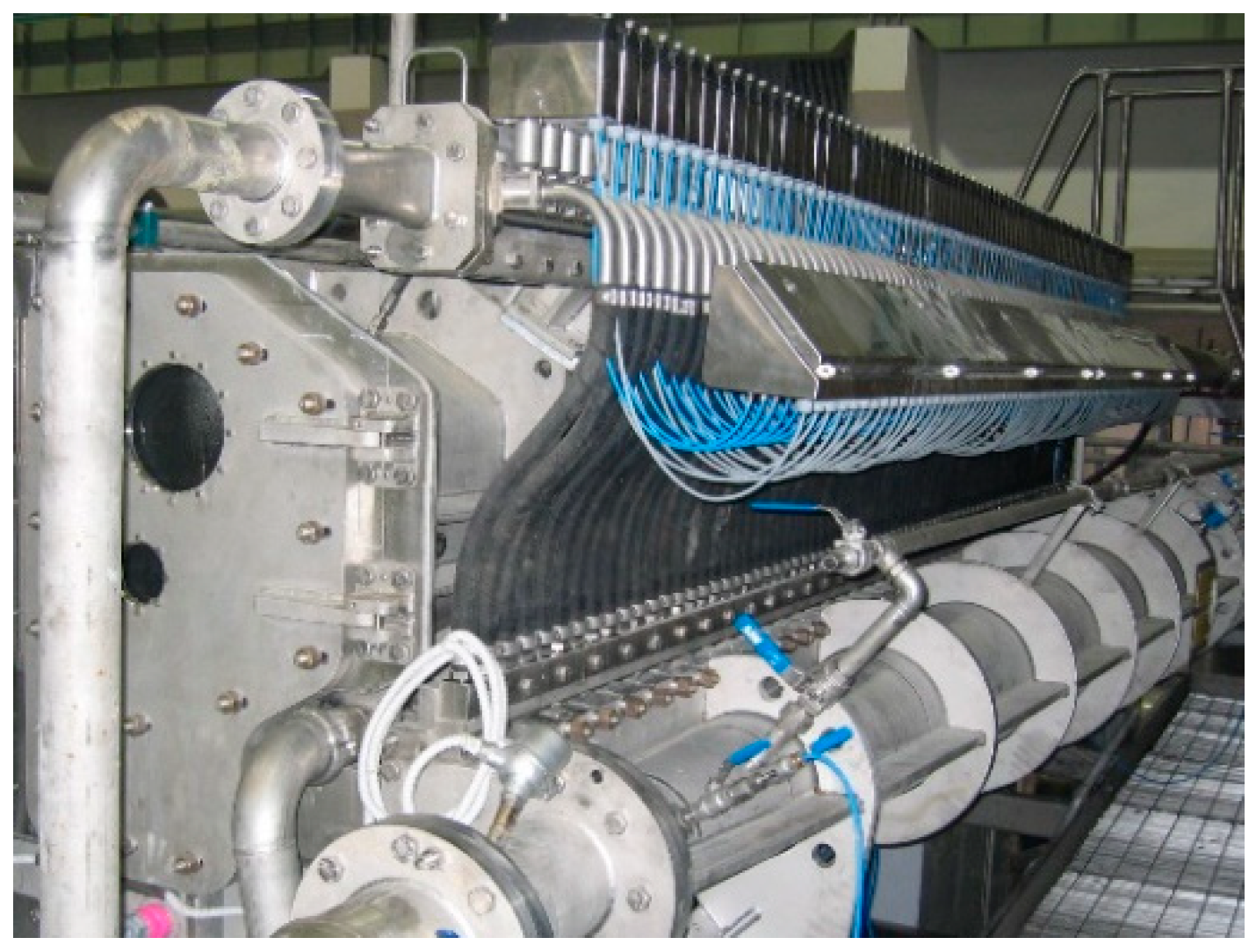
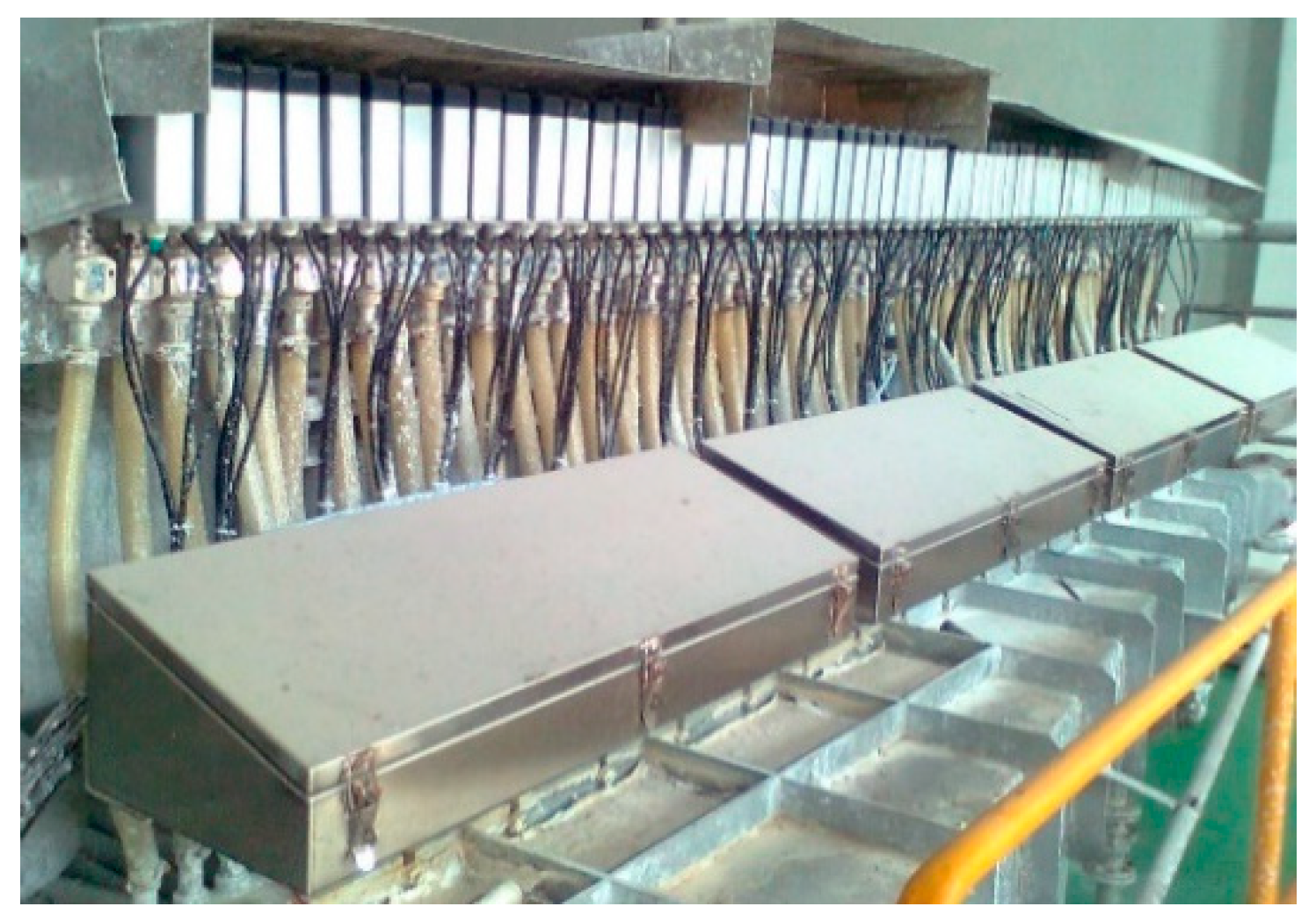
2.1. Materials

The control process is carried out in a hydraulic headbox with diluted water. The operation of the hydraulic headbox is shown in Figure 1. The box body is equipped with glass holes, and the dilution water was colored with red ink so that the flow of fluid from the point of addition to the lip of the headbox can be observed. The dilution water regulating device is shown in Figure 2, which includes a dilution water cone pipe and multiple dilution water valves with automatic control units. One interface of the dilution water valve is connected with the dilution water cone pipe, and the other interface is provided with a water conveying hose that is connected to the pulping branch pipe. The amount of white water injected into the pulp is controlled by adjusting the opening of the dilution valve, and the consistency of the pulp can thereby be adjusted, thus realizing the local fine-tuning of the cross-directional basis weight of the paper.

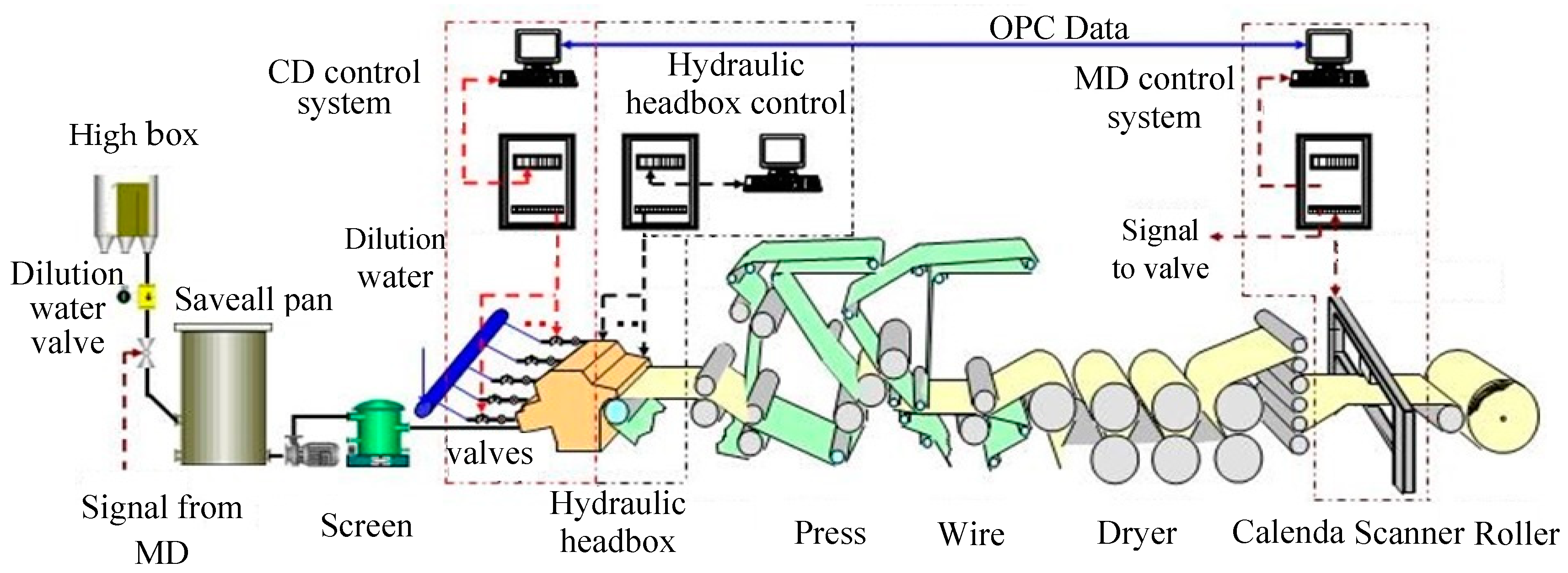
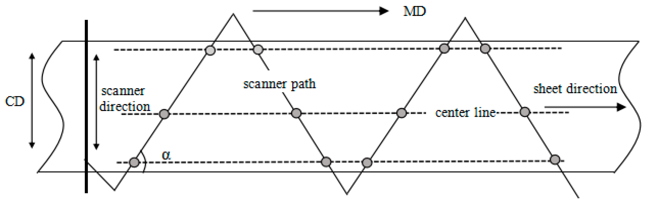
2.2. Measuring Method of the Process Data

The process of CD control for a Fourdrinier machine equipped with a hydraulic headbox is shown in Figure 3. A scanning frame, located between the calender and the winder of the paper machine, supports the basis weight on-line detecting device that scans the paper sheet that moves through the opening of the frame. The system continuously obtains the instantaneous sample value of the basis weight along the machine direction and its CD profiles. These measurements can only be made on paper that is dry enough at the end of the line. This causes a long time delay between the actuators on the hydraulic headbox and measurements from the scanner at the end of the paper machine.

The dilution actuator set-points are determined by the weight profile obtained from the scanning weight sensor. Control actions are based on the profile estimates, which are calculated from the measurements provided by the scanning sensor. The scanner and sensor interface collects analog sensor and scanner data from the basis weight measurement system and builds the basis weight profile to suit the paper machine and actuator requirements.

The sheet typically moves at a velocity on the order of 10 m/s, while the sensors travels back and forth across the paper web at speed from 0 to 1 m/s. This change is usually measured by installing a gauge on a frame so that the gauge can be scanned back and forth throughout the process. When the sheet passes under the gauge, the measured track follows the zig-zag path, as shown in Figure 4, where the angle ‘$\alpha$’ may be only approximately 1°. The horizontal parts in the path correspond to the scanner remaining at the paper edge for a few seconds before changing the direction. Moreover, the gauge stops at one side of the sheet (for unpredictable time intervals) for recalibrating itself. From this sparse data, the whole profile can be reconstructed.

The experimental process was carried out in a paper mill in Wugong city, Shaanxi Province of China in September 2019. The CD basis weight on-line measurement is applied in the paper machine 12 (PM 12), the width of the PM 12 is 5400 mm, and the design speed is 650 m/min. PM 12 produces corrugated paper. In this paper mill, the data of paper basis weight is obtained by a QCS (Quality Control System) through scanning sensors. The data exchange between the OPC (OLE (Object Linking and Embedding) for Process Control) toolbox and the configuration software of WinCC is carried out by MATLAB. The control algorithm is based on the data obtained by MATLAB. The results of the calculations are fed back to WinCC. A S7-300 PLC is adopted for the controller implementation. The interface is driven by an industry standard PLC and provides the programming flexibility to adapt to most measurement systems. The transmission of profiles to the operator station is done through industrial Ethernet communication. The PLC (Programmable Logic Controller) and supporting electronics form a compact unit for ease of installation and maintenance.

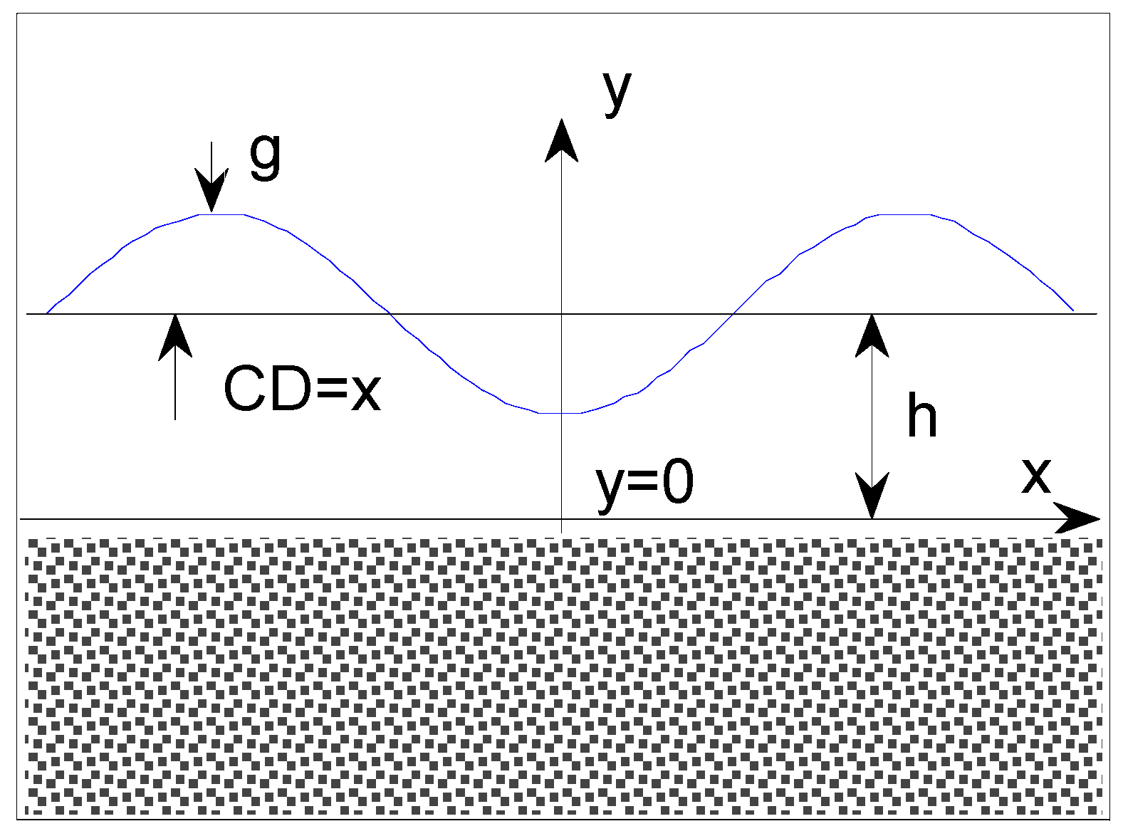
3. Modeling and Block Decomposition of CD Control System

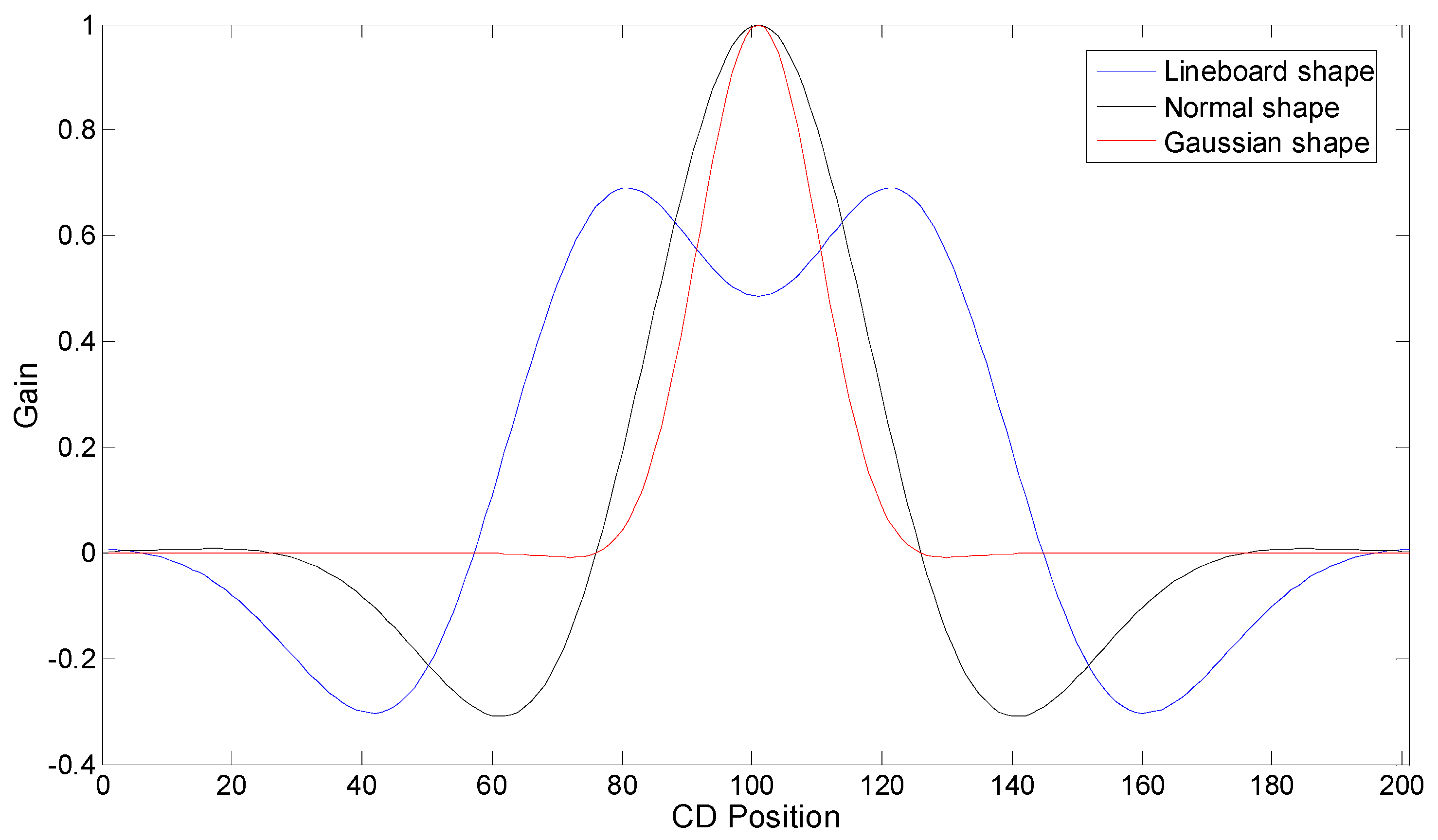
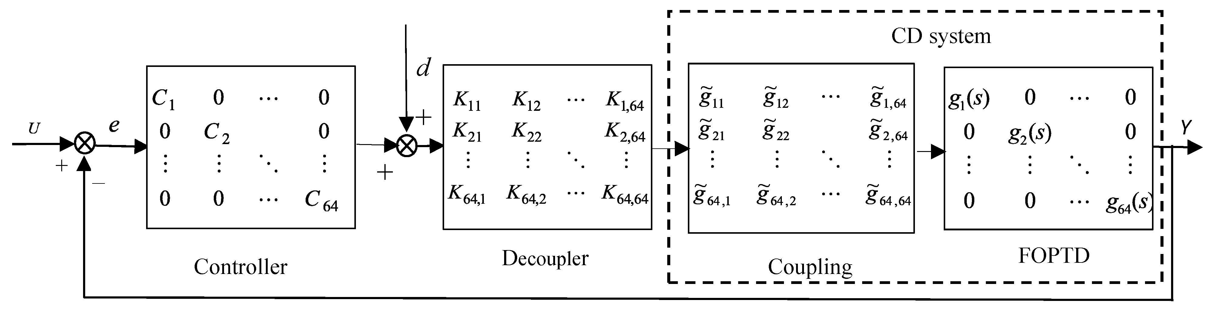
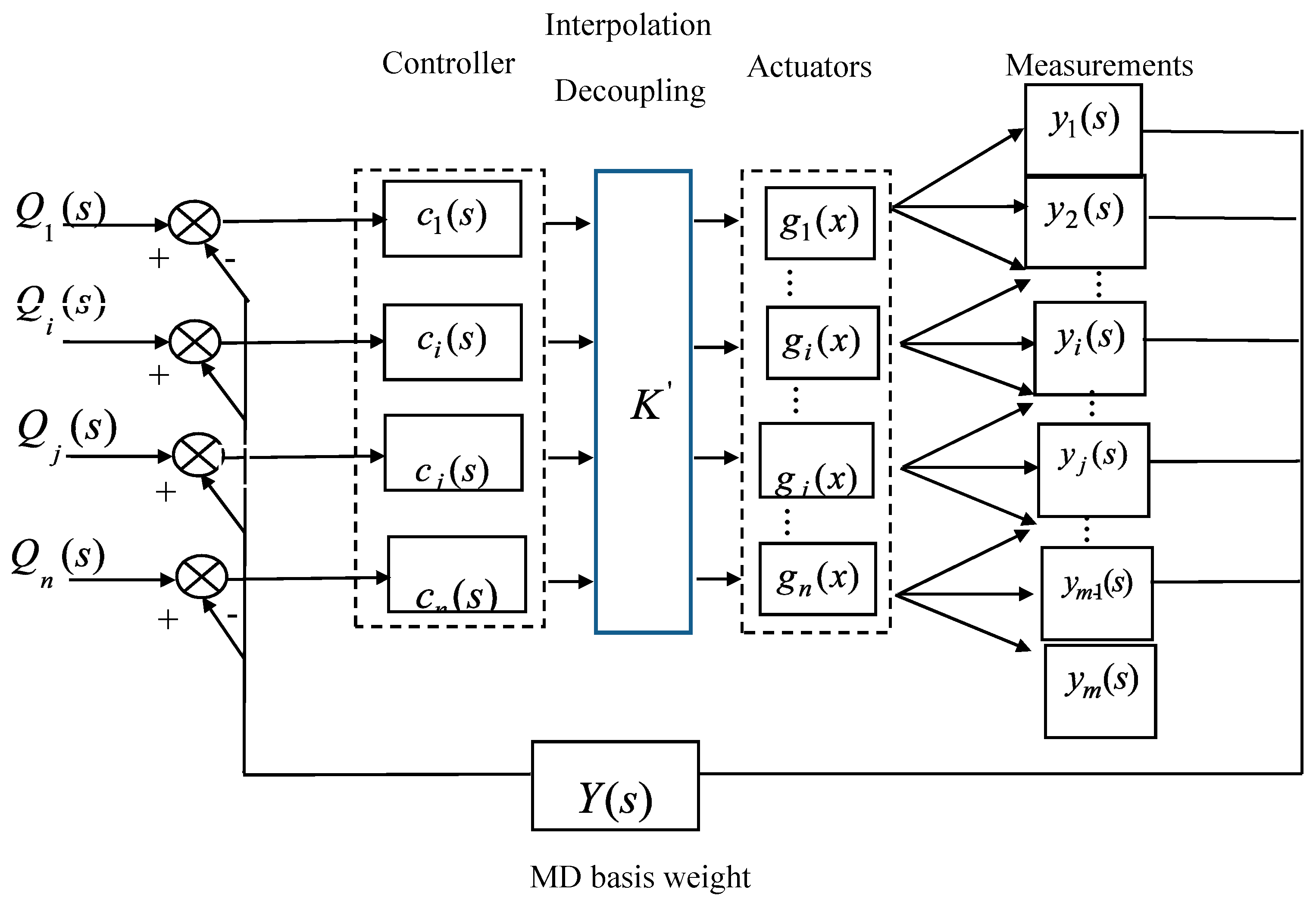
3.1. Modeling of CD Control System

The mathematical model of the CD control system is typically formed as follows: the CD process, i.e., the actuator input–output relationship, is described with a fixed, approximate non-square interaction matrix model, usually assuming identical and equally spaced actuators. It is further assumed that the response is separable, and therefore, the dynamic response of the CD actuator set can be described with a scalar first-order plus delay model. For the different actuator sets, the width of the actuators differ and their spatial responses are very different. The dynamic responses of the actuator sets vary significantly and are dependent on the machine speed and the distance between the actuating and measurement locations.

Like many other sheet and film processes, the simulation model assumes the first-order plus time delay dynamics between the actuator and the sensor. For the input array to the output array, a Toeplitz symmetric input–output interaction matrix is used.

The standard paper machine CD process model is given by

$$\{\begin{array}{l}Y(s)=G(s)U(s)\\ G(s)=G_{0}h(s)\end{array}$$

(1)

where $Y(s)\in {\mathrm{C}}^m$ and $U(s)\in {\mathrm{C}}^n$ are the measurement profile and the actuator set-point profile, respectively, and $G_0\in R^{m\times n}$ is the spatial interaction coupling matrix that describes the response of the process. It also describes the mapping from the actuators to measurements; each component of the actuator vector $U$ corresponds to a column of $G_0$. $m$ and $n$ are the numbers of sheet properties and controlled actuator arrays, respectively. $G_0$ is a block diagonal matrix whose number of columns is equal to the number of actuators, and the number of rows is equal to the number of measurements, where $g_{ij}$ refers to the influence coefficient of the $j^{th}$ actuator on the $i^{th}$ measurement point. For a typical paper machine, if all the CD drive arrays and all the control characteristics are included in a control system, there may be up to 600 individual drives and 6000 profile measurements. In other words, the dimensions of most group process models $G(s)$ in Equation (1) could be 6000 × 600. $h(s)$ is the first-order-plus-time-delay transfer function of the process, and $\tau$ is a delay time of the process. The expressions of $Y(s)$, $U(s)$, $G_0\in R^{m\times n}$, and $h(s)$ are as follows.

$$Y(s)=\left[\begin{array}{c}{y}_1(s)\\ y_2(s)\\ ⋮\\ y_{\mathrm{m}}(s)\end{array}\right],U(s)=\left[\begin{array}{c}{u}_1(s)\\ u_2(s)\\ ⋮\\ u_{\mathrm{n}}(s)\end{array}\right],G_0=\left[\begin{array}{cccc}{g}_{11}& g_{12}& \dots & g_{1n}\\ g_{21}& g_{22}& \ddots & ⋮\\ ⋮& \ddots & \ddots & ⋮\\ g_{m1}& \dots & \dots & g_{mn}\end{array}\right]\begin{array}{l},\\ h(s)=\frac{1}{Ts+1}{\mathrm{e}}^{-\tau \mathrm{s}}\end{array}$$

(2)

The model is based on three assumptions related to in-compressible fluid, irrotational flow, and small amplitude waves. As shown in Figure 5, the static CD profile of the sheet is a two-dimensional wave. Amplitude is a function of position x and time t. It shows the pulp with surface waves on the wire. The x-axis shows the CD, and the y-axis shows the thickness of the pulp.

The origin of the coordinate system is placed at the interface of the fluid and the bed(wire). The wire represents the porous bed. The amplitude of the wave is shown as g, and the mean value is shown as h.

In order to establish the spatial CD responses model, edge effects are studied based on the actuator response model of lip adjustment. The process of establishing the response model of the lip adjustment process is as follows.

For abscissa value x (measuring point position) and ordinate value (time) y, assume that $\eta (x,t)$ is the function of the “S” type wave of the CD deviation profile.

Regarding the assumptions outlined above, the slurry flow is analyzed according to the incompressible fluid. The conservation of mass on a surface “S” that surrounds the incompressible moving fluid implies the continuity equation.

$$\nabla u=0$$

(3)

It implies that the sum of the velocity gradients in any direction should be zero. Assuming an irrotational flow, then the velocity potential $\varphi$ exits, the gradient of which is the velocity of the fluid, and the continuity Equation (3) reduces to a Laplace equation:

$$\frac{{\partial }^2\varphi }{\partial x^2}+\frac{{\partial }^2\varphi }{\partial y^2}=0.$$

(4)

Newton’s second law of motion is then applied to fluid inside “S”

$$\frac{Dq}{Dt}=-\frac{1}{\rho }\nabla P+g.$$

(5)

The boundary condition at the surface is

$$\{\begin{array}{l}y=\eta (x,t)\\ \frac{\partial \eta }{\partial t}-u_y=0,\underset{}{}\mathrm{at}\underset{}{}y=\eta \end{array}.$$

(6)

The dynamic boundary condition is

$$\frac{\partial \varphi }{\partial t}+\frac{1}{2}{q}^2+g\eta +\frac{p_{\eta }}{\rho }=Const\mathrm{at}y=\eta .$$

(7)

After linearizing the dynamic boundary condition, Equation (7) can be simplified as

$$\{\begin{array}{l}-\frac{\partial \phi }{\partial t}+g\eta =0,\underset{}{}\mathrm{at}\underset{}{}y=\eta \\ -\frac{\partial \phi }{\partial t}=u_y\\ P_f=P_b,\underset{}{}\mathrm{at}\underset{}{}y=0\end{array}.$$

(8)

Finally, the function of the “S” type wave of the CD deviation profile can be solved by a multi-objective model.

The objective functions are

$$\{\begin{array}{l}\frac{{\partial }^2\varphi }{\partial x^2}+\frac{{\partial }^2\varphi }{\partial y^2}=0\\ {\nabla }^2{P}_b=0\end{array}.$$

(9)

The boundary conditions are

$$\{\begin{array}{l}y=\eta (x,t)\\ \frac{\partial \eta }{\partial t}-u_y=0\\ \frac{\partial \phi }{\partial t}+\frac{1}{2}{q}^2+g\eta +\frac{p_{\eta }}{\rho }=Const\\ -\frac{\partial \phi }{\partial t}+g\eta =0,\underset{}{}\mathrm{at}\underset{}{}y=\eta \\ -\frac{\partial \phi }{\partial t}=u_y\\ P_f=P_b\end{array}.$$

(10)

The boundary condition is used to separate variables. Consider the following form of surface disturbance.

$$\eta (x,t)=A_0{\mathrm{e}}^{\mathrm{j}(N_x-\omega t)}$$

(11)

The real part of the Equation (11) is only considered

$$\eta (x,t)=A_0{\mathrm{e}}^{-k_{d}x}\cos (kx-\omega t).$$

(12)

When the CD profile does not vary with time,

$$\eta (x,0)=A_0{\mathrm{e}}^{-k_{d}x}\cos kx.$$

(13)

The response modeling method and identification method of the slice lip actuator (continuum device) and dilution actuator (discrete device) are similar.

So, the response model of the dilution water valve of $g(x,t)$ has a similar form of expression with $\eta (x,t)$. As the CD basis weight does not vary with time, $g(x,t)$ can be simplified to $g(x)$. For a continuous sheet-forming process, the relationship between the two-dimensional sheet change $g(x)$ and CD control action to the $j^{th}$ CD actuator can be expressed as Equation (14).

$$g(x)=\frac{r}{2}\{{\mathrm{e}}^{\frac{-\alpha {(x+\beta \xi )}^2}{{\xi }^2}}\cos [\frac{\pi (x+\beta \xi )}{\xi }]+{\mathrm{e}}^{\frac{-\alpha {(x-\beta \xi )}^2}{{\xi }^2}}\cos [\frac{\pi (x-\beta \xi )}{\xi }]\}$$

(14)

It is shown that the spatial response of a single controller can be represented by the extension of a set of orthogonal functions, where the spatial coordinate $x$ is a scalar real number, $\gamma$ is a gain parameter, and $\zeta$ is a width parameter. The parameters $\gamma$ and $\zeta$ define the linear transformation of the response by stretching it vertically and horizontally, respectively. The attenuation parameter $\alpha$ changes the size of the negative lobes of the response. The divergence parameter $\beta$ defines the presence of two maxima in the response and the distance between these two maxima.

The shape of the spatial response represented by Equation (14) is illustrated in Figure 6. For the line board shape, $r=1$, $\xi =20$, $\alpha =1.5$, and $\beta =0$. For the normal shape, $r=2.5$, $\xi =20$, $\alpha =1.5$, and $\beta =0.4$. For the Gaussian shape, $r=1$, $\xi =40$, $\alpha =1.5$, and $\beta =0.4$.

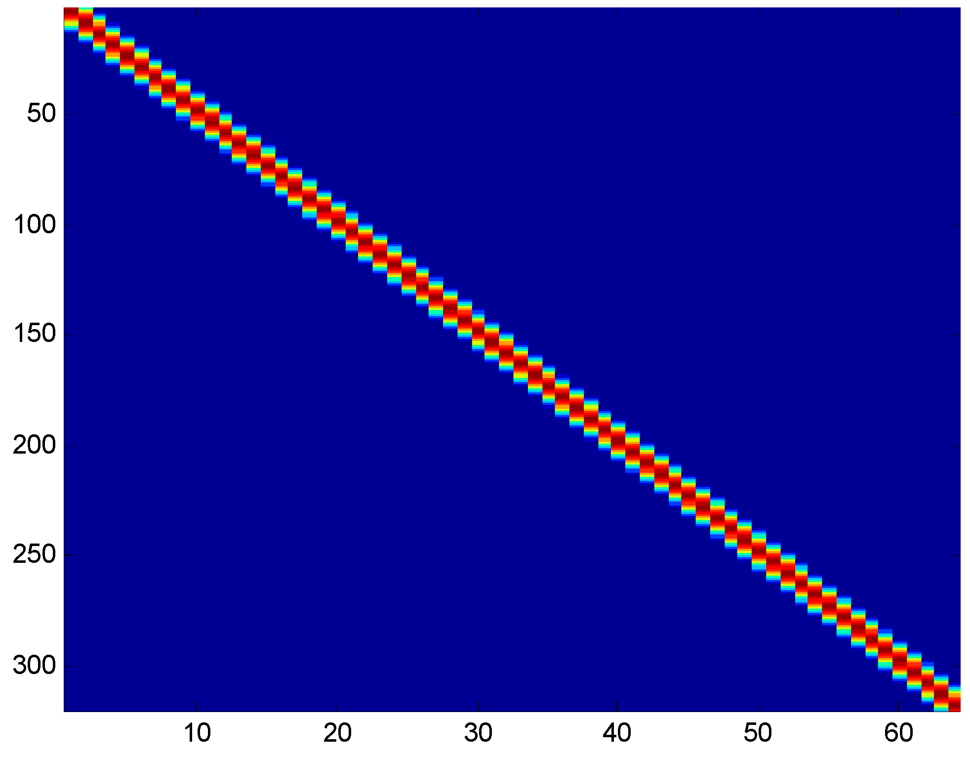
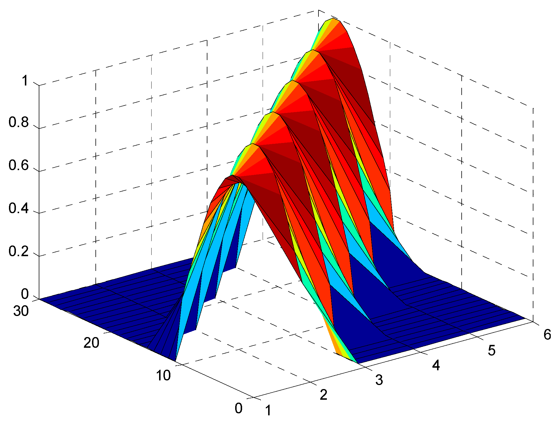
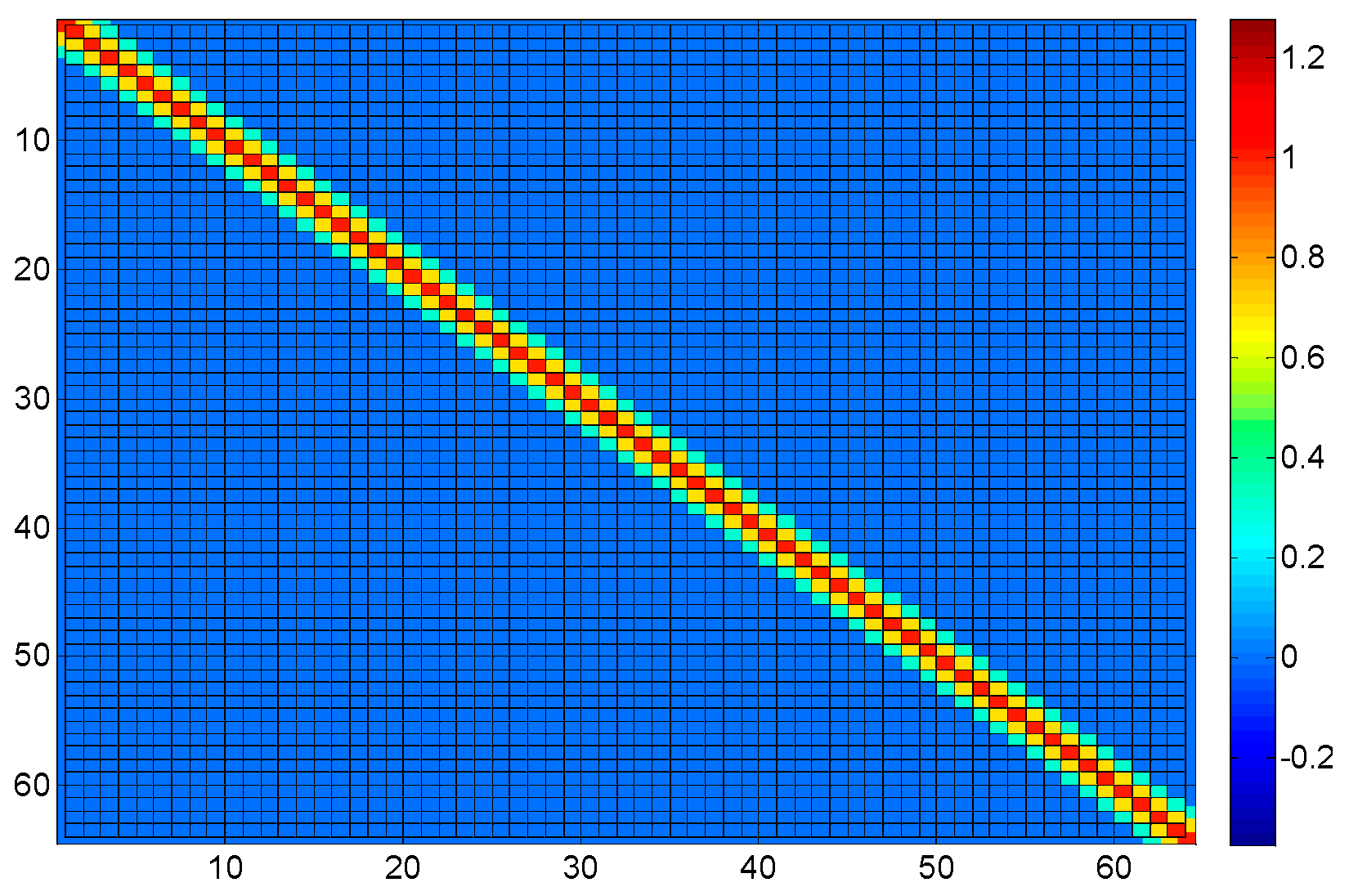
3.2. Identification of Coupling Matrix

In the CD control system, the measured dimension $m$ is usually much higher than that of the actuator setpoints dimension $n$ (generally, $3n<m<10n$). In the experimental simulation, taking a dilution water hydraulic headbox with 64 dilution water valves as an example, the measurements and the actuator form a large-scale interaction coupling matrix with dimensions of $320\times 64$. Experiments have shown that when a single dilution water valve is operated, the affected area includes 26 measured data points on both sides of the valve [8].

The number of measurements is an integer multiple of the number of actuators in this example, such as $m=5\times n$, which means that one actuator maps to five measured data points. Each actuator affects 26 measured data points on each side. The actuator has the strongest influence on the measured data point at the downstream position, and the coupling coefficient is the largest. As the distance increases, the impact will gradually decrease. If there are more than 26 lateral intervals, the effect is weak [9]. The mapping relationship between the actuators and the measured data is shown in Figure 7, where the solid line indicates the greatest impact, and the dotted line indicates the gradual weakening.

Based on such an example, a large-scale interaction coupling matrix $G_0$ can be described as shown in Equation (15). The parameters $g_1,\cdots ,g_{26}$ describe the spatial response of the process, where 26 is the half-width of the response of one actuator and $m$ represents the scanning space between adjacent actuators.

$$G_0=\left[\begin{array}{ccccccc}{g}_1& g_6& g_{11}& \cdots & g_{26}& 0& \cdots \\ g_2& g_5& g_{10}& \cdots & g_{25}& 0& \cdots \\ g_3& g_4& g_9& \cdots & g_{24}& 0& \cdots \\ g_4& g_3& g_8& \cdots & g_{23}& 0& \cdots \\ g_5& g_2& g_7& \cdots & g_{22}& 0& \cdots \\ g_6& g_1& g_6& \cdots & g_{21}& g_{26}& \cdots \\ g_7& g_2& g_{11}& \cdots & g_{20}& g_{25}& \cdots \\ ⋮& ⋮& ⋮& \ddots & ⋮& ⋮& ⋮\\ g_{26}& g_{21}& g_{16}& \cdots & g_1& g_6& \cdots \\ 0& g_{22}& g_{17}& \cdots & g_2& g_5& \cdots \\ 0& g_{23}& g_{18}& \cdots & g_3& g_4& \cdots \\ 0& g_{24}& g_{19}& \cdots & g_4& g_3& \cdots \\ 0& g_{25}& g_{20}& \cdots & g_5& g_2& \cdots \\ 0& g_{26}& g_{21}& \cdots & g_6& g_1& \cdots \\ ⋮& ⋮& ⋮& \ddots & ⋮& ⋮& ⋮\\ 0& 0& g_{25}& \cdots & g_{10}& g_5& \cdots \\ 0& 0& g_{26}& \cdots & g_{11}& g_6& \cdots \\ ⋮& ⋮& ⋮& \ddots & ⋮& ⋮& ⋮\\ 0& 0& 0& 0& 0& 0& \cdots \end{array}\right]\in R^{m\times n}$$

(15)

As the number of $n$ actuators in the system, the process model can be given by

$$G_0=[\overline{g_1},\overline{g_2}\cdots ,\overline{g_n}]\in {\mathrm{R}}^{m\times n}$$

(16)

where one of the columns $\overline{g_j}\in {\mathrm{R}}^m$ represents the sample space response of the $j^{th}$ actuator, which is determined by

$$\overline{g_j}(x)=g(x-c_j).$$

(17)

$c_j$ is the measured data coordinate of the spatial response centre for the $j^{th}$ actuator.

Based on the Gaussian shape, the coupling matrix $G_0$ can be calculated. $G_0$ is a sparse strip matrix with a large number of zero elements (see Figure 8), where the non-zero data reflect the coupling coefficient of each CD position and the strip width reflects the strength of the coupling. Figure 9 and Figure 10 show the non-zero data distribution. It can be seen that the elements on the main diagonal are larger, and the remaining elements are small. This indicates that $G_0$ is a non-square, high-dimensional, symmetric interaction matrix with small-range coupling characteristics.

As the symmetric inherent in the physical architecture of the web forming processes [10], the structure of a Toeplitz symmetric matrix is usually illustrated in the interaction matrix $G_0$. The same constant element is repeated along each diagonal of the matrix in a Toeplitz symmetric matrix. The constant square band–diagonal interaction matrix $G_0$ with m independent spatial coupling partials in Equation (15) can be expressed as a Toeplitz symmetric matrix: $G_0={\mathrm{Toeplitz}(\mathrm{g}}_1,\cdots {,\mathrm{g}}_{\mathrm{m}},0,\cdots ,0)$.

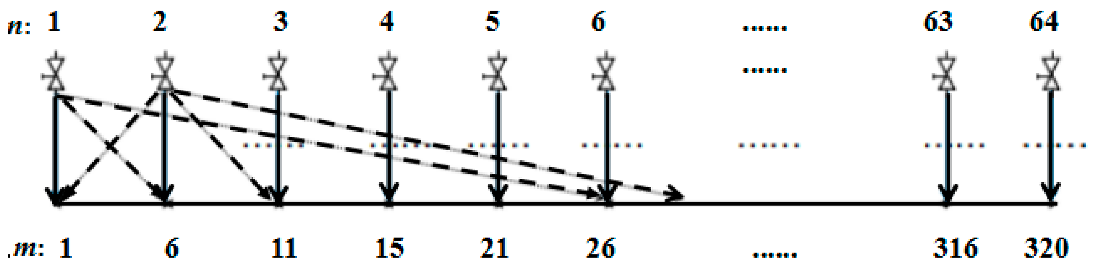
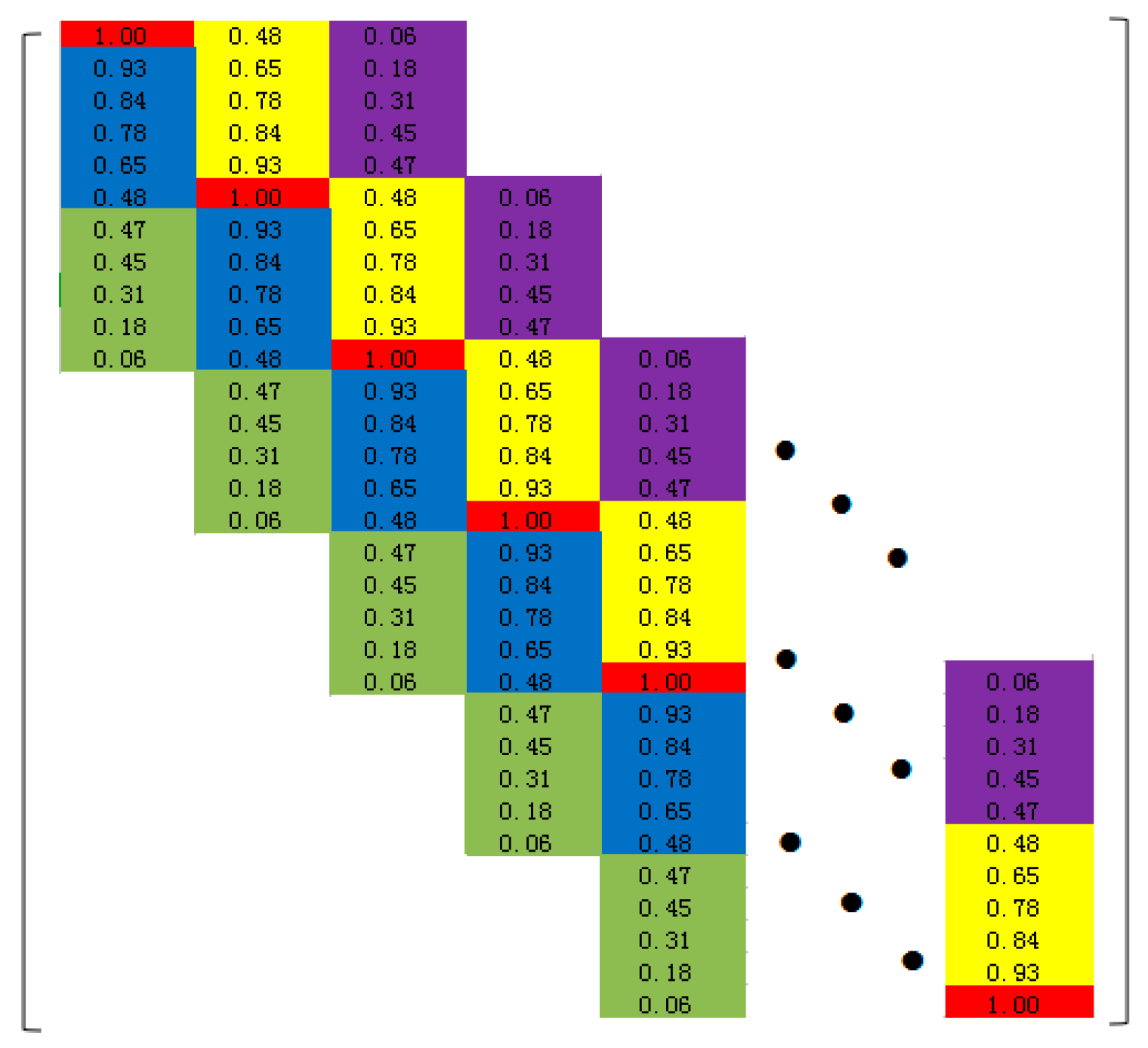
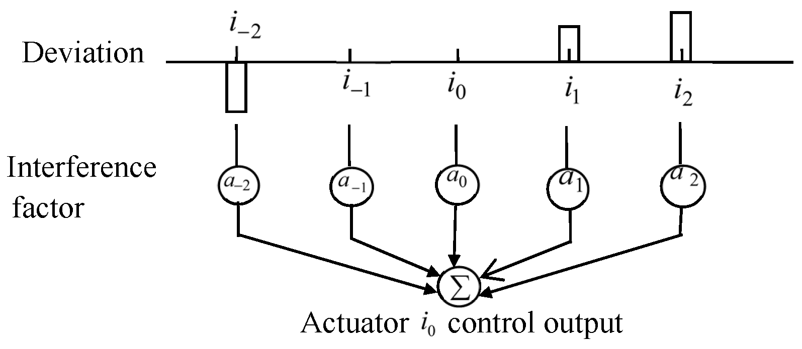
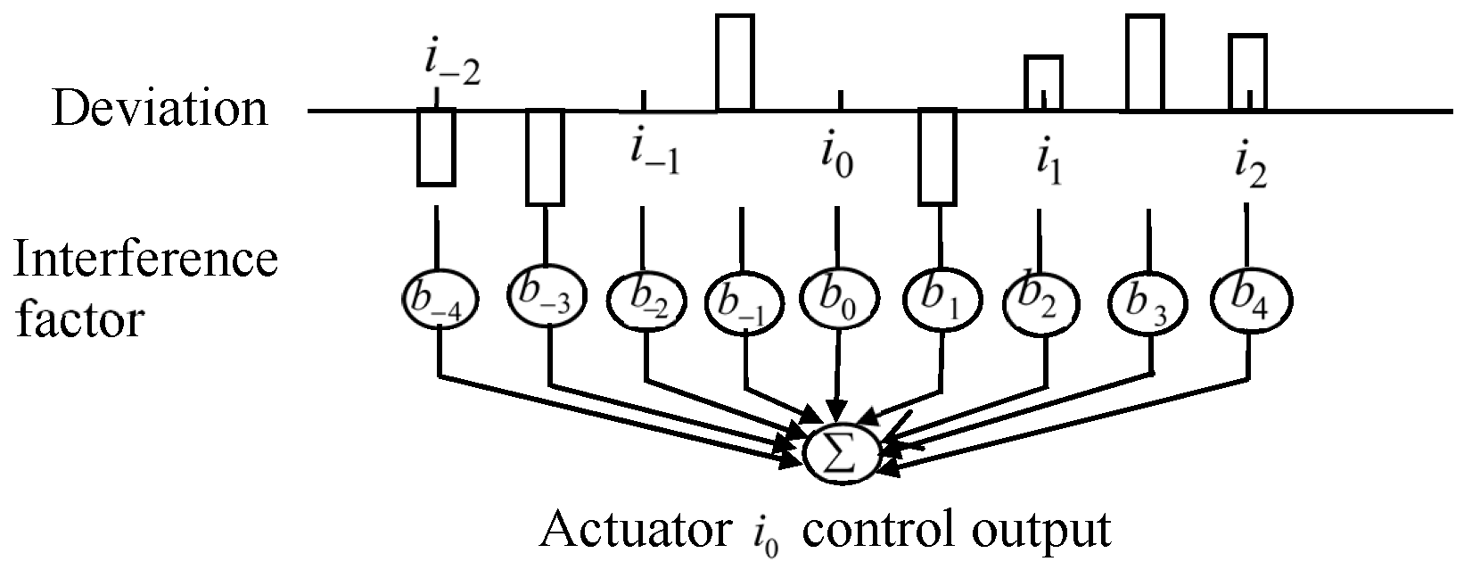
3.3. Block and Decomposition Control of Coupling Matrix

For non-square high-dimensional coupling systems, it is necessary to adopt a suitable method to reduce the system dimension and convert it into a square system for decoupling. According to the strip coupling width of the above interaction matrix, $G_0$ is standardized as shown in Figure 11, where $p$ is the coupling width, which indicates the number of affected actuators on the adjacent side when adjusting an actuator ($p=2$ in this paper), and $2p+1$ is the strip width.

3.3.1. Coupling Matrix Blocking

For simplifying the analysis, a blocking-based triangulation strategy is adopted for the coupling matrix $G_0$. Along the diagonal, the coupling matrix can be divided into $q\times q$ block matrices. Thus, a new block gain matrix of ${\widehat{G}}_0$ can be partitioned as

$${\widehat{G}}_0={\left[\begin{array}{ccccc}{G}_2& G_1{}^T& 0& \cdots & 0\\ G_1& G_2& G_1{}^T& \ddots & ⋮\\ 0& \ddots & \ddots & \ddots & 0\\ ⋮& \ddots & G_1& G_2& G_1{}^T\\ 0& \cdots & 0& G_1& G_2\end{array}\right]}_{q\times q}$$

(18)

where $q=\left[\frac{m}{2p+1}\right]=\left[\frac{320}{2\times 2+1}\right]=64$ and [ ] is the rounding up function; for example; for example, [H] represents the smallest integer, which is no less than H [11]. $G_1$ is an upper triangular $(2p+1)\times (2p+1)$ matrix, and $G_2$ is a symmetric $(2p+1)\times (2p+1)$ matrix. The structures of $G_1$ and $G_2$ are given by

$$G_1={\left[\begin{array}{ccccc}0& 0& g_p& \cdots & 0\\ 0& 0& \ddots & \ddots & ⋮\\ ⋮& \ddots & \ddots & \ddots & g_p\\ ⋮& & \ddots & 0& 0\\ 0& \cdots & \cdots & 0& 0\end{array}\right]}_{(2p+1)\times (2p+1)},G_2={\left[\begin{array}{ccccc}{g}_0& \cdots & g_p& \cdots & 0\\ ⋮& \ddots & ⋮& \ddots & ⋮\\ g_p& \cdots & g_0& \cdots & g_p\\ ⋮& \ddots & ⋮& \ddots & ⋮\\ 0& \cdots & g_p& \cdots & g_0\end{array}\right]}_{(2p+1)\times (2p+1)}.$$

(19)

For the new block gain matrix of ${\widehat{G}}_0$, the output variables are different from the original output of $Y(s)$. The new CD process model is shown in Equation (20).

$$\widehat{Y}(s)={\widehat{G}}_{0}h(s)U(s)$$

(20)

where $\widehat{Y}(s)\in {\mathrm{C}}^{\mathrm{n}}$ and $U(s)\in {\mathrm{C}}^{\mathrm{n}}$, $\widehat{Y}(s)$ indicates the low-dimensional measurement profile obtained by transformation matrix of $F$.

$$\widehat{Y}(s)=FY(s)=\left[\begin{array}{cccc}{f}_{11}& f_{12}& \cdots & f_{1m}\\ f_{21}& f_{22}& \cdots & f_{2m}\\ ⋮& ⋮& \ddots & ⋮\\ f_{n1}& f_{n2}& \cdots & f_{nm}\end{array}\right]\left[\begin{array}{c}{y}_1(s)\\ y_2(s)\\ ⋮\\ y_{\mathrm{m}}(s)\end{array}\right]$$

(21)

Based on such a division, the original CD control system with the dimensions of $m\times n$ is divided into $q$ groups, and each group contains $2p+1$ subsystems, where the model of the subsystem can be expressed as

$${\widehat{Y}}_j(t)=h(z^{-1})[\underset{1}{\underbrace{G_2{\hat{u}}_j(t-\mathsf{\tau })}}+\underset{2}{\underbrace{G_1{\hat{u}}_{j-1}(t-\mathsf{\tau })}}+\underset{3}{\underbrace{G_1{}^{\mathrm{T}}{\hat{u}}_{j+1}(t-\mathsf{\tau })}}]+E(t).$$

(22)

For the $j^{th}$ subsystem, ${\widehat{Y}}_j(t)$ is the output of the measurement profile at time t. These measurements can only be made on paper that is dry enough at the end of the line. This causes a long time delay between the actuators on the hydraulic headbox and measurements from the scanner at the end of the paper machine. ${\hat{u}}_j(t-\tau )$ is the input of the $j^{th}$ CD actuator set-point profile at $t-\tau$ time. $u_{j-1}(t-\tau )$ and $u_{j+1}(t-\tau )$ represent the ${(j-1)}^{th}$ and ${(j+1)}^{th}$ CD actuator set-point profile at $t-\tau$ time. $E(t)$ is the noise sequence. The symmetric parts of 2 and 3 in Equation (22) correspond to the paper CD basis weight boundaries. The block matrix $G_1$, $G_1{}^{\mathrm{T}}$ is located at the boundary of the interaction matrix, and $G_2$ is located on the main diagonal of the interaction matrix. When the effect controlled by $G_2$ is non-zero and the other parts of the control effect are zero, $G_0$ can be converted to a main diagonal matrix. Then, the system can be simplified as a main diagonal system, and the coupling can be reduced. Based on the input variable adjustment, the decomposition algorithm is adopted to eliminate the control effect of sub-blocks 2 and 3 in this paper.

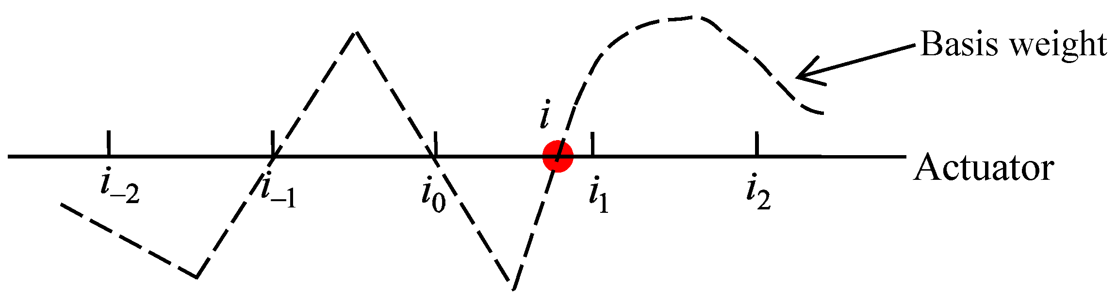
3.3.2. Decomposition Algorithm Control

By a blocking-based triangulation strategy, $q$ multivariable subsystems that have dimensions of $2p+1$ are obtained. To eliminate the edges of each subsystem, a decomposition algorithm is adopted in this part. The decomposition algorithm steps are as follows.

Divide the control variables into groups according to the horizontal position, each group containing five control points.

Construct a new constraint applied to the control input $U$.

The construction principle of the new constraint is that the control action cannot be applied to all the actuators in the same group at the same time [12], such as that the $u_j$ actuator cannot be set for simultaneous actions in subsystem $j$, although the actuators in different groups can be set simultaneously.

At one moment, each actuator rotates in a sequence of Equation (23):

$$[u_1,0,\cdots ,0],[0,u_2,0,\cdots ,0],[0,\cdots ,0,u_i,0,\cdots ,0],[0,\cdots ,0,u_{2p+1}].$$

(23)

Cyclically input the control variables in chronological order. Actuators belonging to different groups can act simultaneously [13]. For example, from the time of $t$ to $t+2p+1$, the following constraints are imposed on each subsystem control input, as shown in

Table 1. The form of the subsystem control input.

Time	$\mathbf{Control}\mathbf{Input}{\mathit{u}}_1$	$\mathbf{Control}\mathbf{Input}{\mathit{u}}_2$	$\cdots$	$\mathbf{Control}\mathbf{Input}{\mathit{u}}_{\mathit{q}-1}$	$\mathbf{Control}\mathbf{Input}{\mathit{u}}_{\mathit{q}}$
$t$	${\left[u_{1,}0,\cdots ,0\right]}^T$	${\left[0,\cdots ,0,u_{p,}0,\cdots ,0\right]}^T$	$\cdots$	${\left[u_{1,}0,\cdots ,0\right]}^T$	${\left[0,\cdots ,0,u_{p,}0,\cdots ,0\right]}^T$
$t+1$	${\left[0,u_{2,}0,\cdots ,0\right]}^T$	${\left[0,\cdots ,0,u_{p+1,}0,\cdots ,0\right]}^T$	$\cdots$	${\left[0,u_{2,}0,\cdots ,0\right]}^T$	${\left[0,\cdots ,0,u_{p+1,}0,\cdots ,0\right]}^T$
$⋮$	$⋮$	$⋮$	$⋮$	$⋮$	$⋮$
$t+p+1$	${\left[0,\cdots ,0,u_{p,}0,\cdots ,0\right]}^T$	${\left[0,\cdots ,0,u_{2p+1}\right]}^T$	$\cdots$	${\left[0,\cdots ,0,u_{p,}0,\cdots ,0\right]}^T$	${\left[0,\cdots ,0,u_{2p+1}\right]}^T$
$⋮$	$⋮$	$⋮$	$⋮$	$⋮$	$⋮$
$t+2p+1$	${\left[0,\cdots ,0,u_{2p+1}\right]}^T$	${\left[u_{1,}0,\cdots ,0\right]}^T$	$\cdots$	${\left[0,\cdots ,0,u_{2p+1}\right]}^T$	${\left[u_{1,}0,\cdots ,0\right]}^T$

.

The non-zero element of the control input $u(t)$ is shifted circularly. By reasonably arranging the cyclic order in adjacent subsystems, the associated impact can be minimized.

Based on the real mapping matrix method introduced by Duncan [14], the transformation matrix of $F$ can be simplified as described in Equation (24). The Equation (21) can be described in Equation (25).

$$F=\left[\begin{array}{cccc}{f}_{11}& f_{12}& \cdots & f_{1m}\\ f_{21}& f_{22}& \cdots & f_{2m}\\ ⋮& ⋮& \ddots & ⋮\\ f_{n1}& f_{n2}& \cdots & f_{nm}\end{array}\right]={\left[\begin{array}{cccccccccc}\frac{1}{5}& \cdots & \frac{1}{5}& 0& \cdots & 0& \cdots & 0& \cdots & 0\\ 0& \cdots & 0& \frac{1}{5}& \cdots & \frac{1}{5}& \cdots & 0& \cdots & 0\\ ⋮& \cdots & ⋮& ⋮& \cdots & ⋮& \ddots & ⋮& \cdots & ⋮\\ 0& \cdots & 0& 0& \cdots & 0& \cdots & \frac{1}{5}& \cdots & \frac{1}{5}\end{array}\right]}_{64\times 320}$$

(24)

$$\begin{array}{c}{\left[\begin{array}{cccccccccc}\frac{1}{5}& \cdots & \frac{1}{5}& 0& \cdots & 0& \cdots & 0& \cdots & 0\\ 0& \cdots & 0& \frac{1}{5}& \cdots & \frac{1}{5}& \cdots & 0& \cdots & 0\\ ⋮& \cdots & ⋮& ⋮& \cdots & ⋮& \ddots & ⋮& \cdots & ⋮\\ 0& \cdots & 0& 0& \cdots & 0& \cdots & \frac{1}{5}& \cdots & \frac{1}{5}\end{array}\right]}_{64\times 320}\times {\left[\begin{array}{c}{y}_1(s)\\ y_2(s)\\ ⋮\\ y_m(s)\end{array}\right]}_{320\times 1}\\ \begin{array}{l}\\ ={\left[\begin{array}{cccccccccc}\frac{1}{5}& \cdots & \frac{1}{5}& 0& \cdots & 0& \cdots & 0& \cdots & 0\\ 0& \cdots & 0& \frac{1}{5}& \cdots & \frac{1}{5}& \cdots & 0& \cdots & 0\\ ⋮& \cdots & ⋮& ⋮& \cdots & ⋮& \ddots & ⋮& \cdots & ⋮\\ 0& \cdots & 0& 0& \cdots & 0& \cdots & \frac{1}{5}& \cdots & \frac{1}{5}\end{array}\right]}_{64\times 320}\end{array}\times {\left[\begin{array}{cccc}{g}_{11}& g_{12}& \dots & g_{1n}\\ g_{21}& g_{22}& \ddots & ⋮\\ ⋮& \ddots & \ddots & ⋮\\ g_{m1}& \dots & \dots & g_{mn}\end{array}\right]}_{320\times 64}\times {\left[\begin{array}{c}{u}_1(s)\\ u_2(s)\\ ⋮\\ u_{\mathrm{n}}(s)\end{array}\right]}_{64\times 1}\times \frac{1}{Ts+1}{\mathrm{e}}^{-\tau \mathrm{s}}\end{array}$$

(25)

During the period from $t$ to $t+2p+1$, efficient control inputs $[u_1,u_2,\cdots ,u_q](q=64)$ are applied to the $320\times 64$ CD system. Based on these control inputs, the original high-dimensional non-square CD control system with the dimensions of $320\times 64$ can be converted to a new low-dimensional CD system with the dimensions of $64\times 64$, which can be described as shown in Equation (26).

$$\left[\begin{array}{c}{\widehat{Y}}_1(s)\\ {\widehat{Y}}_2(s)\\ ⋮\\ {\widehat{Y}}_{64}(s)\end{array}\right]={\left[\begin{array}{cccc}{G}_{11}& G_{12}& \dots & G_{1n}\\ G_{21}& G_{22}& \ddots & ⋮\\ ⋮& \ddots & \ddots & ⋮\\ G_{n1}& \dots & \dots & G_{nn}\end{array}\right]}_{64\times 64}\times \left[\begin{array}{c}{u}_1(s)\\ u_2(s)\\ ⋮\\ u_{64}(s)\end{array}\right]\times \frac{1}{Ts+1}{\mathrm{e}}^{-\tau \mathrm{s}}$$

(26)

For the new low-dimensional square system, the interaction matrix with a number of dimensions equal to the number of actuators and a one-to-one correspondence between the CD measuring point and the actuator is solved. The new interaction matrix ${\tilde{G}}_0$ can be given as follows

$${\tilde{G}}_0={\left[\begin{array}{cccccccc}1& 0.7& 0.3& & & & & \\ 0.7& 1& 0.7& 0.3& & & & \\ 0.3& 0.7& 1& 0.7& \ddots & 0.3& & \\ & 0.3& 0.7& 1& \ddots & 0.7& 0.3& \\ & & 0.3& 0.7& \ddots & 1& 0.7& 0.3\\ & & & 0.3& \ddots & 0.7& 1& 0.7\\ & & & & & 0.3& 0.7& 1\end{array}\right]}_{64\times 64}.$$

(27)

Moreover, the new interaction matrix ${\tilde{G}}_0$ is a Toeplitz symmetric matrix. ${\tilde{G}}_0=Toeplitz(f)$ [15], where $f=[1,0.7,0.3,0\cdots 0]$.

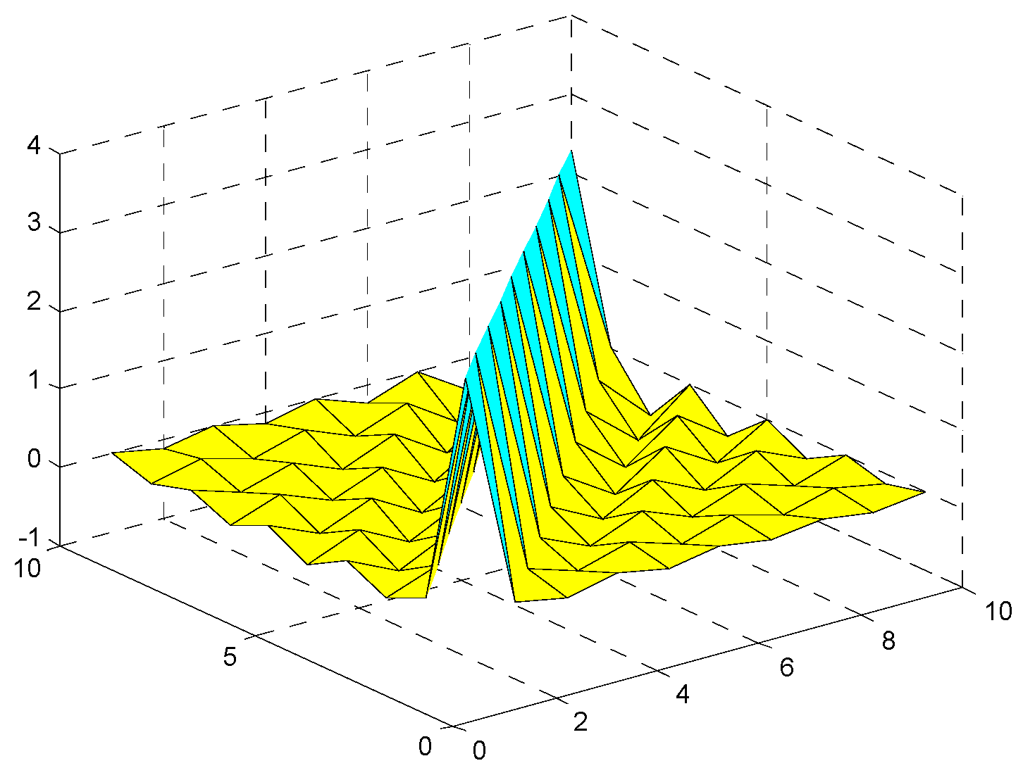
4. Interpolation Decoupling Strategy for CD Control System

For the high-dimensional Toeplitz symmetric interation matrix with small-scale coupling characteristics, a decoupling network is added between the controller and the controlled object. By the decoupling network, the controlled object is transformed into a principal diagonally dominant system. The control structure with a decoupler is shown in Figure 12.

The coupling matrix is a static matrix, which does not change with time. Then, the decoupler is also a static matrix [16]. For the new associated coupling matrix obtained above, the generalized inverse of a 64-dimensional Toeplitz matrix can be calculated. The product of a matrix and its adjoint matrix is a diagonal matrix in mathematics; that is,

$${\tilde{G}}_0\times adj({\tilde{G}}_0)=adj({\tilde{G}}_0)\times {\tilde{G}}_0=\det ({\tilde{G}}_0)\times I.$$

(28)

From the point of view of simplified design, the decoupler can be designed as

$$K=adj({\tilde{G}}_0).$$

(29)

The detailed structure is shown in Equation (30).

$$K={\left[\begin{array}{ccccccc}2.028& -1.715& 0.572& \cdots & -2.381& 0.572& 0.315\\ -1.715& 3.429& -2.286& \cdots & 4.984& -2.952& 0.572\\ 0.572& -2.286& 3.429& \cdots & -3.693& 4.984& -2.381\\ ⋮& ⋮& ⋮& \ddots & ⋮& ⋮& ⋮\\ -2.381& 4.984& -3.693& \cdots & 3.429& -2.286& 0.572\\ 0.572& -2.952& 4.984& \cdots & -2.286& 3.429& -1.715\\ 0.315& 0.572& -2.381& \cdots & 0.572& -1.715& 2.029\end{array}\right]}_{64\times 64}$$

(30)

It can be seen that the decoupling matrix of $K$ is a 64-dimensional symmetric matrix, and each element is not zero. Then, the number of decoupling network branches that need to be calculated is 64 $\times$ 64/2 = 2048, and the decoupling speed is slower with the increase of the system dimensions. In order to achieve fast decoupling of the controlled system, it is necessary to further analyze the system and simplify the decoupling network.

The number of basis weight measurements is typically about 360, and the number of actuators is about 64 (i.e., five data per actuator). In order to reduce the number of calculated measurements, the corresponding deviation of each actuator is obtained by averaging the corresponding five data.

However, the average for each actuator may not catch a peak if there is one between the actuators (see Figure 13, the dilution valve $i$ exists between $i_0$ and $i_1$). In this case, the dilution valve is interpolated, and the more dilution valves that are interpolated, the smaller the control deviation after the decoupling matrix. Based on the coupling matrix mentioned above, the interpolation matrix method is proposed to decouple the coupling system quickly.

It is assumed that a point of the dilution water valve is inserted in each equidistant area to obtain twice the number of dilution water valves. Strictly, (twice the number of actuators-1). Compared with the control method of the decoupling matrix in Figure 14, the average section width of the control deviation is halved, as shown in Figure 15. Then, the peak value of the basis weight profile between the actual actuators has a great impact on the average control deviation [17]. In addition, the size of the interference factor matrix is also doubled. This control deviation technique by the interpolated decoupling matrix is named the ‘Interpolated Decoupling Matrix Method’ [18].

For the output of the dilution valve actuator $U(s)={[u_1(s),u_2(s),\cdots ,u_n(s)]}^{\mathrm{T}}$, assuming the output of the $i_0{}^{th}$ dilution valve is $u_i{}_0$, when the $i_0{}^{th}$ dilution valve operates, it is necessary to adjust the opening of the left and right dilution valves in a certain proportion, while for the $i_0{}^{th}$ region, there is a combined control regulation. The output $u_i{}_0$ of the $i_0{}^{th}$ dilution valve can be expressed as

$$u_i{}_0={\displaystyle \sum _{\mathrm{j}=-2}^2{a}_j}{P}_j$$

(31)

where $a_j$ is the interference factor obtained for each existing actuator. $P_j$ is the control variable obtained from control deviation by the PI (Proportion-Integral) controller for each existing actuator.

In the interpolated decoupling matrix method, the coupling factor matrix is twice the original. The output $u_i{}_0$ of the $i_0{}^{th}$ dilution valve is expressed as follows.

$$u_i{}_0={\displaystyle \sum _{\mathrm{j}=-4}^4{b}_j}{P}_j{}^{\prime }$$

(32)

where $b_j$ is the interference factor obtained for the actuator, assuming that the number of actuators is equal to the number of actual actuators $\times$2. $P_j^{\prime }$ is the manipulated variable obtained from control deviation, assuming that the number of actuators is equal to twice the number of actual actuators.

After the interpolation input of the controller, when the opening of the dilution valve changes, the influence on the left and right sides of the slurry flow will be reduced [19]. Therefore, the correlation matrix can be further transformed into a new weak coupling correlation matrix ${\stackrel{⌢}{G}}_0$, which is expressed as

$${\stackrel{⌢}{G}}_0={\left[\begin{array}{cccccccc}1& 0.34& 0.16& & & & & \\ 0.34& 1& 0.34& 0.16& & & & \\ 0.16& 0.34& 1& 0.34& \ddots & 0.16& & \\ & 0.16& 0.34& 1& \ddots & 0.34& 0.16& \\ & & 0.16& 0.34& \ddots & 1& 0.34& 0.16\\ & & & 0.16& \ddots & 0.34& 1& 0.34\\ & & & & & 0.16& 0.34& 1\end{array}\right]}_{64\times 64}.$$

(33)

For the new coupling matrix, the new 64-dimensional Toeplitz matrix is singularity judged by $\det ({\stackrel{⌢}{G}}_0)\ne 0$, and the diagonal decoupler can be designed as

$$K^{\prime }=\mathrm{inv}({\stackrel{⌢}{G}}_0).$$

(34)

A new decoupling matrix is obtained by truncating the new decoupling matrix $K^{\prime }$, the value less than ${10}^{-3}$ is approximated to 0, and the banded symmetric matrix $K^{\prime }$ as shown in Equation (35) is obtained.

$$K^{\text{'}=}{\left[\begin{array}{cccccccccccccccc}1.279& -0.374& -0.086& 0.096& -0.016& -0.012& 0.007& & & & & & & & & \\ -0.374& 1.279& -0.347& -0.086& 0.102& -0.016& -0.012& 0.007& & & & & & & & \\ -0.086& -0.347& 1.279& -0.347& -0.116& 0.102& -0.016& -0.012& \ddots & & & & & & & \\ 0.096& -0.086& -0.347& 1.279& -0.347& -0.116& 0.103& -0.016& \ddots & 0.007& & & & & & \\ -0.016& 0.096& -0.086& -0.347& 1.279& -0.347& -0.116& 0.103& \ddots & -0.012& 0.007& & & & & \\ -0.012& -0.016& 0.096& -0.086& -0.347& 1.279& -0.347& -0.116& \ddots & -0.016& -0.012& 0.007& & & & \\ 0.007& -0.012& -0.016& 0.096& -0.086& -0.347& 1.279& -0.347& \ddots & 0.103& -0.016& -0.012& 0.007& & & \\ & 0.007& -0.012& -0.016& 0.096& -0.086& -0.347& 1.279& \ddots & -0.116& 0.103& -0.016& -0.012& 0.007& & \\ & & 0.007& -0.012& -0.016& 0.096& -0.086& -0.347& \ddots & -0.347& -0.116& 0.103& -0.016& -0.012& 0.007& \\ & & & 0.007& -0.012& -0.016& 0.096& -0.086& \ddots & 1.279& -0.347& -0.116& 0.103& -0.016& -0.012& 0.007\\ & & & & 0.007& -0.012& -0.016& 0.096& \ddots & -0.347& 1.279& -0.347& -0.116& 0.103& -0.016& -0.012\\ & & & & & 0.007& -0.012& -0.016& \ddots & -0.086& -0.347& 1.279& -0.347& -0.116& 0.103& -0.016\\ & & & & & & 0.007& -0.012& \ddots & 0.096& -0.086& -0.347& 1.279& -0.347& -0.116& 0.103\\ & & & & & & & 0.007& \ddots & -0.016& 0.096& -0.086& -0.347& 1.279& -0.347& -0.116\\ & & & & & & & & \ddots & -0.012& -0.016& 0.096& -0.086& -0.347& 1.279& -0.347\\ & & & & & & & & & 0.007& -0.012& -0.016& 0.096& -0.086& -0.347& 1.279\end{array}\right]}_{64\times 64}$$

(35)

The non-zero data distribution of $K^{\prime }$ is shown in Figure 16 and Figure 17. It can be shown that the main diagonal elements are larger and the other elements are smaller.

It can be seen that the decoupling network is also a Toeplitz matrix. There are only 436 non-zero branches in the strip of $K^{\prime }$, and the decoupling matrix $K^{\prime }$ is a symmetric matrix. It means that only 186 branches need to be calculated in the process of decoupling calculation. The decoupling branch is greatly reduced, which improves the decoupling speed of the system. This result indicates that the original complex decoupling network is transformed into a simple and easy-to-implement decoupling network based on the interpolation method.

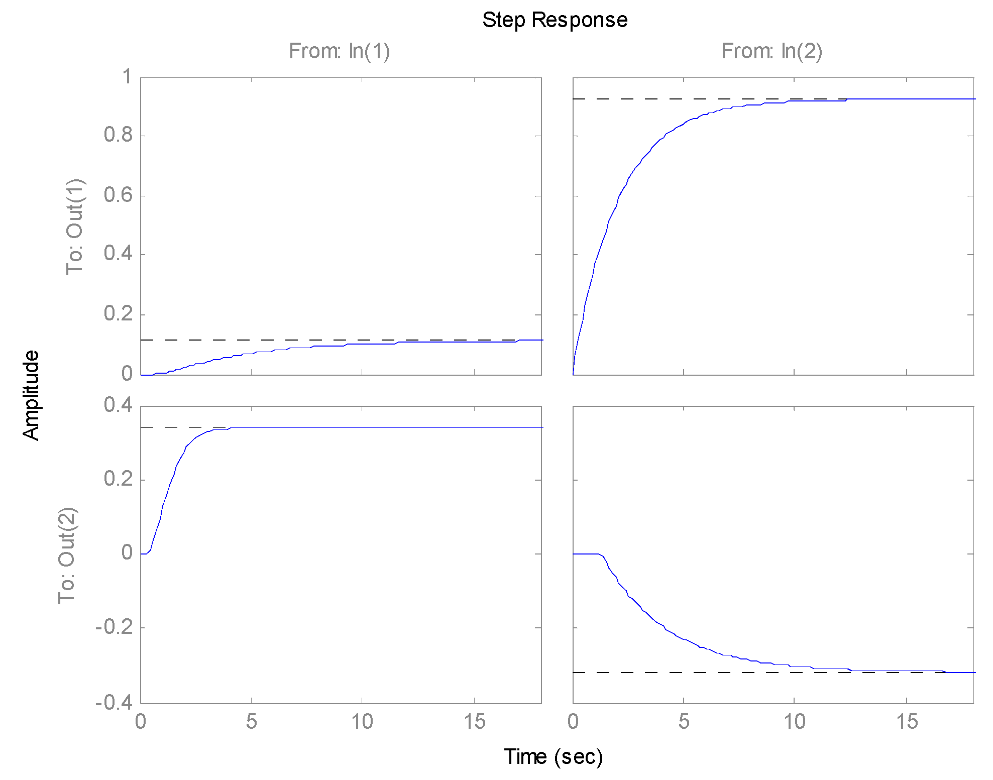
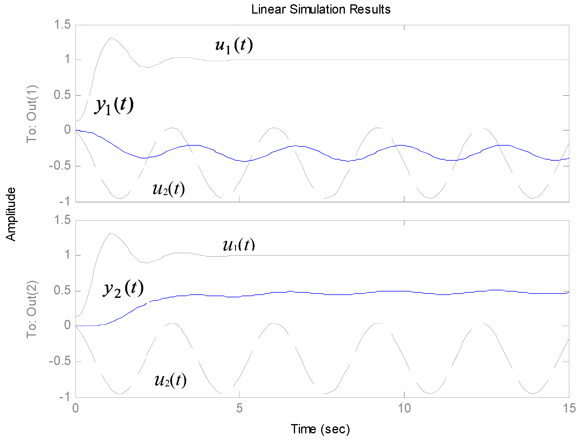
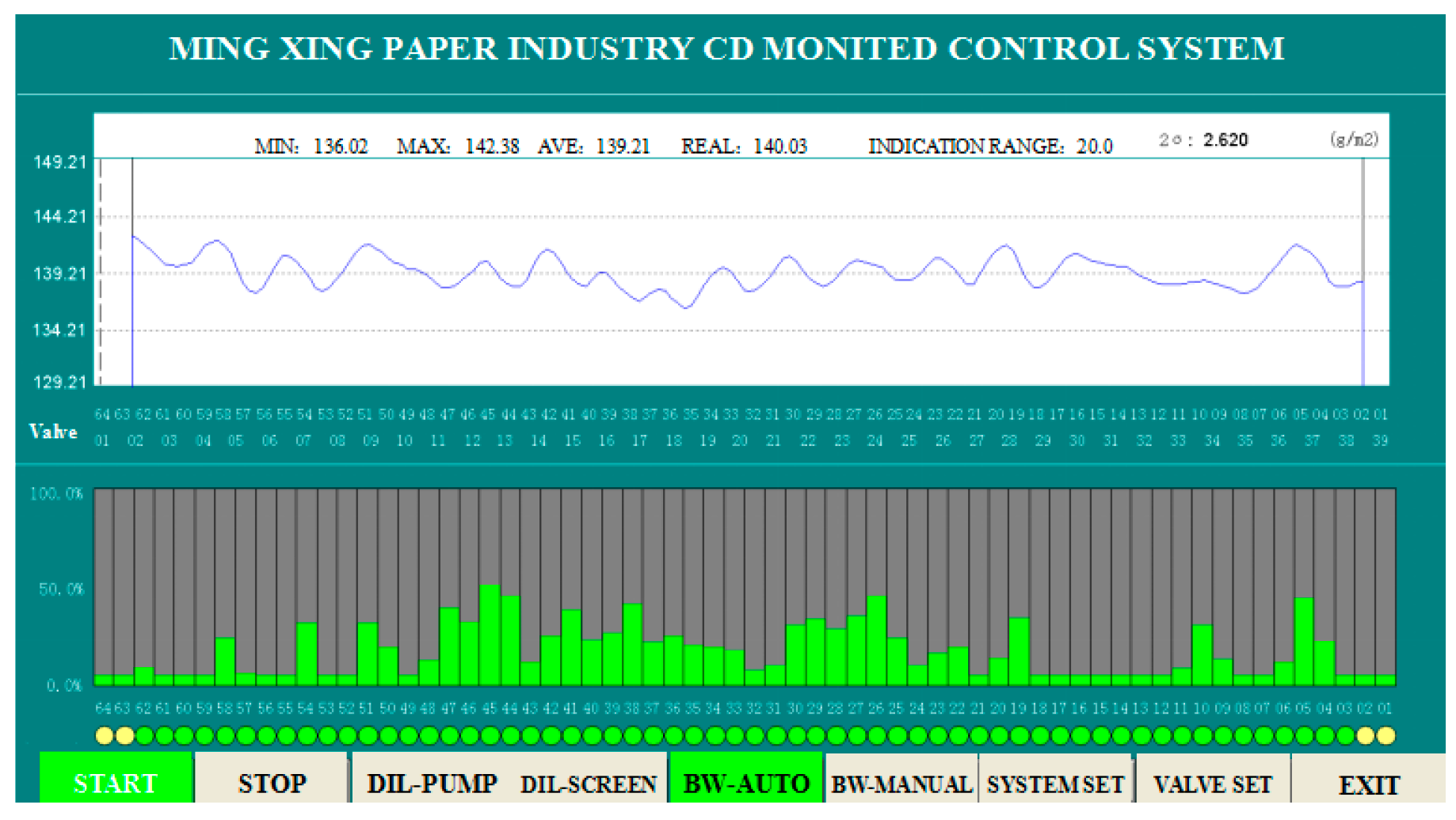
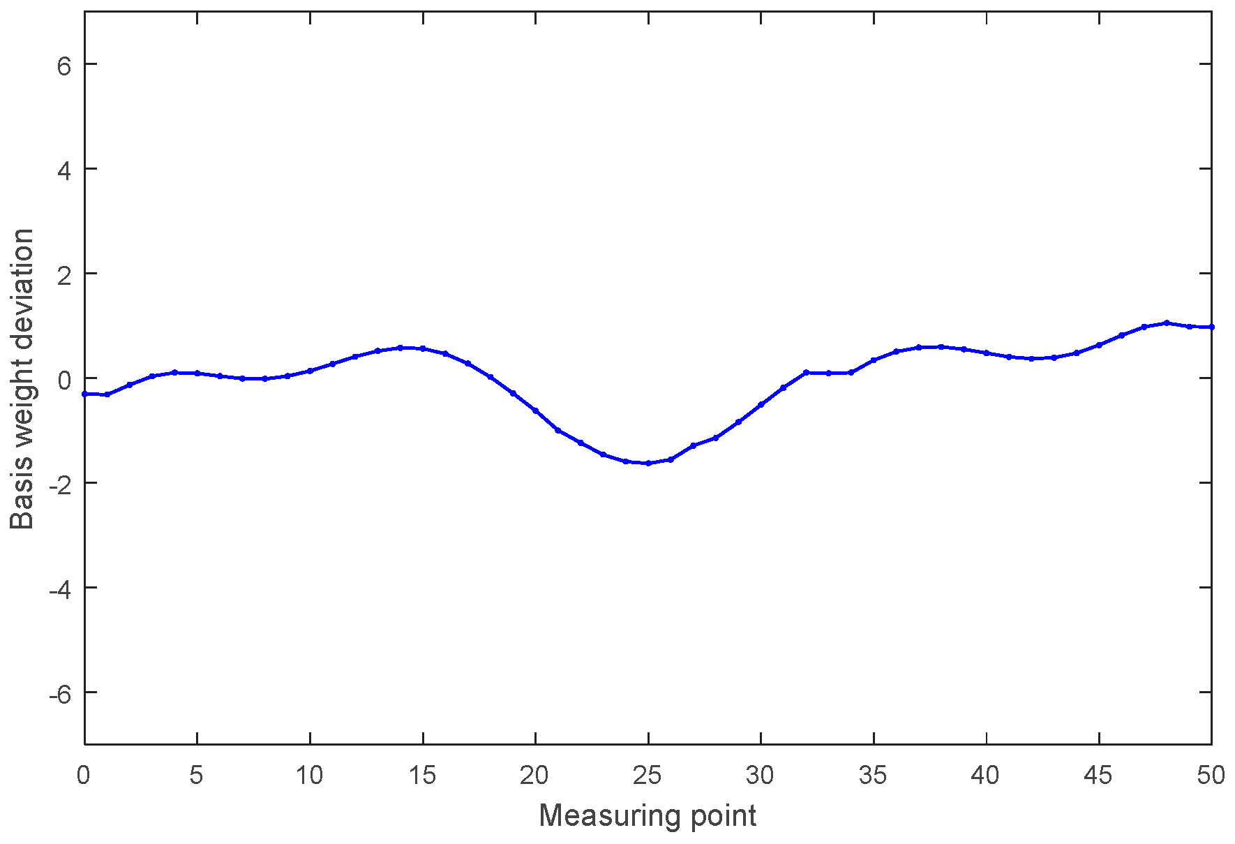
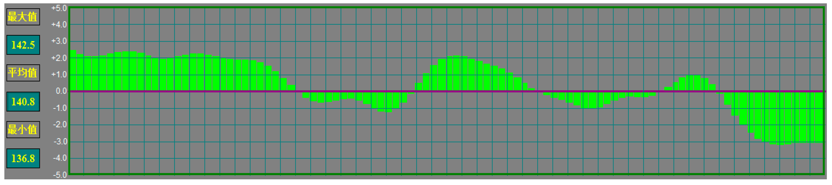
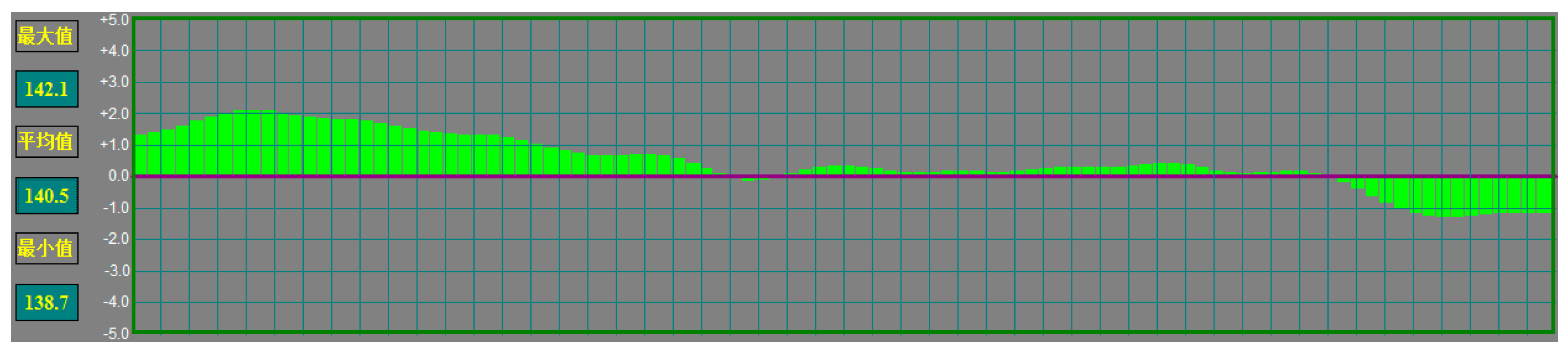
5. Results of Simulation and Application

For the new system with 64 dimensions, there are 64 actuators mapping 64 regions, which means that the coupling between each region is eliminated. Thus, the control of a high-dimensional large-scale system can be transformed into multiple single-loop control. The block diagram of subsystem parallel control is shown in Figure 18.

A decoupled CD control system for corrugated paper with a basis weight of 133 g/m² was implemented in an actual project of a paper mill.

The basis weight of corrugated paper is 140 g/m², and the allowable basis weight fluctuation range is $\pm 7$ g/m². In order to reduce the pulp consumption in the paper production process, the actual project stabilizes the paper basis weight at 133 g/m² for automatic control. Based on the criterion of equal basis weight in each region, the following model is established.

$$\{\begin{array}{l}{g}_{11}{u}_1+g_{12}{u}_2+g_{13}{u}_3=b\\ g_{21}{u}_1+g_{22}{u}_2+g_{23}{u}_3+g_{24}{u}_4=b\\ g_{31}{u}_1+g_{32}{u}_2+g_{33}{u}_3+g_{34}{u}_4+g_{35}{u}_5=b\\ ⋮\\ g_{64,62}{u}_{62}+g_{64,63}{u}_{63}+g_{64,64}{u}_{64}=b\end{array}$$

(36)

where $U=\left[\begin{array}{ccccc}{u}_1& u_2& \cdots & u_{63}& u_{64}\end{array}\right]$ is the output of the dilution valve actuator and $b$ is the normalized setting value of the CD basis weight.

As $rank(\tilde{G})=rank(\tilde{G},b)=64$, there is a unique solution to Equation (36).

$$\begin{array}{l}U=\left[\begin{array}{ccccc}{u}_1& u_2& \cdots & u_{63}& u_{64}\end{array}\right]\\ =[1,0.53,0.02,0.94,0.25,0.23,0.97,0,0.44,0.87,0.24,0.57,0.69,0.51,0.61,0.45,\\ 0.75,0.55,0.17,0.9,0.39,0.07,0.97,0.16,0.32,0.94,0.06,0.5,0.81,0.34,0.59,0.61,\\ 0.61,0.59,0.35,0.81,0.5,0.06,0.94,0.32,0.17,0.97,0.07,0.39,0.9,0.17,0.55,0.75,\\ 0.45,0.61,0.51,0.69,0.57,0.24,0.87,0.44,0,0.97,0.23,0.25,0.94,0.02,0.53,1]\end{array}$$

(37)

According to the calculated regulation of each dilution valve, the opening of the dilution valve is changed as the initial value of the input variable of the control system changes.

In the decoupled CD system, each single loop controlled by 64 actuators has similar physical characteristics. It is the first-order plus time delay (FOPTD) dynamic response of the process. Each loop controller design is relatively simple. Take a two-loop adjustment for example. For each single-loop design controller, the response curve under the action of the controller is shown in Figure 19 and Figure 20. According to the figures, the first-step input produces a good output $y_1(t)$ when applied to the system, and $y_2(t)$ is almost 0. The effect is found to be similar when the second input is used alone. The loops do not affect each other. It is proven that the coupling relationship has been eliminated very well. Moreover, the control quality is improved.

Setting the paper basis weight at 133 g/m², the dilution valves are controlled by the S7-300 PLC. When the working condition is stable, a monitoring picture of a certain period is shown in Figure 21, and 50 scanning points are measured randomly. The basis weight deviation curve is shown in Figure 22. It can be seen that the fluctuation deviation is small, so that the algorithm is proven to be very practical.

To further verify the effectiveness of the algorithm, a low-dimensional CD system was set up in the experiment, with the CD measured data points $m=24$ and the number of dilution valves being the same as m ($n=m$). The coupling width of the interaction matrix was 2, and the basis weight fluctuations after the decoupling control were compared. As shown in Figure 23 and Figure 24, it can be seen that the basis weight fluctuation range is significantly reduced, and the product quality is improved based on the decoupling control strategy.

6. Conclusions

In view of the characteristics of strong multivariable coupling in a cross-directional (CD) basis weight control system, a conventional decoupling control strategy may be difficult to meet the actual needs of a CD basis weight control system. Thus, it is necessary to study the effective decoupling or compensation control strategy. In this paper, a general method of transforming the control problem of a high-dimensional large-scale system into a single-loop group control problem is proposed based on the matrix block method and the interpolation decoupling strategy. Based on a model of the CD basis weight profile, the coupling properties of a CD control system are analyzed by numerical simulation. The matrix block method and model reduction were applied in the interaction coupling matrix of dimensions of $320\times 64$, and the original $320\times 64$ non-square CD control system can be converted to a new low-dimensional CD system with dimensions of only $64\times 64$. For the 64-dimensional Toeplitz symmetric subsystem with small-scale coupling characteristics, an interpolation decoupling algorithm is adopted, and then a decoupling compensator with the structure of a symmetric Toeplitz matrix was obtained. Based on the multi-actuator parallel control strategy, a decoupled multivariable system is achieved. The coupling calculation in this paper is based on the data collected from the actual paper mill. An interpolation decoupling controller is designed to transform an MIMO system into multiple SISO systems. Experimental results show that the method has an obvious decoupling control effect, and this control strategy can provide help for the actual project. In addition, the multidimensional interpolation decoupling control strategy and a real-time decomposition algorithm can be applied to various processes whose input and output numbers are different.

References

- Gorinevsky, M.; Stein, G. Structured Uncertainty Analysis of Robust Stability for Multidimensional Array Systems. IEEE Trans. Autom. Control 2003, 48, 1557–1568. [Google Scholar] [CrossRef]
- Fukumine, H.; Miura, F. Control Parameter Optimization Service for Paper Machine Quality Control Systems, QCS Tune-up Engineering, for Ideal Paper Manufacturing Plant. In Yokogawa Technical Report English Edition; Media Publications: Tokyo, Japan, 2011; Volume 54, pp. 61–64. Available online: https://www.yokogawa.com/th/library/resources/yokogawa-technical-reports/control-parameter-optimization-service-for-paper-machine-quality-control-systems-qcs-tune-up-engineering-for-ideal-paper-manuf/ (accessed on 8 January 2020).
- Stewart, G.E.; Gorinevsky, D.M.; Dumont, G.A. Feedback Controller Design for a Spatially Distributed System: The Paper Machine Problem. IEEE Trans. Control Syst. Technol. 2003, 11, 612–622. [Google Scholar] [CrossRef]
- Gorinevsky, M.; Gheorghe, C. Identification Tool for Cross-directional Processes. IEEE Trans. Control Syst. Technol. 2003, 11, 629–638. [Google Scholar] [CrossRef]
- Gheorghe, C.; Lahouaoula, A.; Chu, D.L. Multivariable CD Control with Adaptive Alignment for a High-production Linerboard Machine. J. Sci. Technol. For. Prod. Process. 2012, 2, 32–42. [Google Scholar]
- Toro, R.; Martínez, C.O.; Logist, F.; Impe, J.V.; Puig, V. Tuning of Predictive Controllers for Drinking Water Networked Systems. In Proceedings of the 18th IFAC World Congress, Milano, Italy, 28 August–2 September 2011. [Google Scholar]
- Ohenoja, M.; Leiviska, K. Multiple Property Cross Direction Control of Paper Machine. Model. Identif. Control 2011, 32, 103–111. [Google Scholar] [CrossRef][Green Version]
- Morales, R.M.; Heath, W.P. The Robustness and Design of Constrained Cross-directional Control via Integral Quadratic Constraints. IEEE Trans. Control Syst. Technol. 2011, 19, 1421–1432. [Google Scholar] [CrossRef]
- Chen, S.C.; Naimimohasses, R.; Zehnpfund, A. Improving Reel-building with Multivariable CD Control. In Proceedings of the Paper Conference and Trade Show: Growing in the Future, New Orleans, LA, USA, 22–25 April 2012. [Google Scholar]
- Amma, M.E.; Dumont, G.A. Identification of Paper Machines Cross-directional Models in Closed-loop. Model. Identif. Control 2013, 3, 245–256. [Google Scholar]
- Featherstone, A.P.; VanAntwerp, J.G.; Braatz, R.D. Cross-Directional Control, 1st ed.; Springer: London, UK, 2000. [Google Scholar]
- Sadighi, A.; Ahmad, A.; Irandoukht, A. Modeling a Pilot FixedBed Hydrocracking Reactor via a Kinetic Base and Neuro-Fuzzy Method. J. Chem. Eng. Jpn. 2010, 43, 174–185. [Google Scholar] [CrossRef]
- Malashenko, A. The Dilution Control Headbox. Pap. Technol. 1997, 12, 42–53. [Google Scholar]
- Hansen, O. MasterJet II—For Super Sheet Formation. Voith Pap. 2008, 25, 24–32. [Google Scholar]
- Jiang, W. Practical Experience of Headbox Rebuilding. China Pulp Pap. 2010, 11, 67–70. [Google Scholar]
- Lin, C. Research and Development of the Key Technology of MC Dilution Hydraulic Headbox. China Pulp Pap. 2010, 29, 56–61. [Google Scholar]
- Shi, X. Observer-based fuzzy adaptive control for multi-input multi-output nonlinear systems with a nonsymmetric control gain matrix and unknown control direction. Fuzzy Sets Syst. 2015, 23, 1–26. [Google Scholar] [CrossRef]
- Dave, P.; Willing, D.A.; Kudva, G.K.; Pekny, J.F.; Doyle, F.J. LP Methods in MPC of Large-Scale Systems: Application to Paper-Machine CD Control. AIChE J. 1997, 43, 1016–1031. [Google Scholar] [CrossRef]
- Jeremy, G.; Andrew, P.; Richard, D. Robust Cross-directional Control of Large Scale Sheet and Film processes. J. Process. Control 2011, 11, 149. [Google Scholar]