Article

LCA/LCC Model for Evaluation of Pump Units in Water Distribution Systems

1
Faculty of Technical Sciences, Department for Industrial Engineering and Management, University of Novi Sad, 21000 Novi Sad, Serbia
2
Faculty of Technical Sciences, Department for Mechanical Engineering, University of Novi Sad, 21000 Novi Sad, Serbia
*
Author to whom correspondence should be addressed.
Symmetry 2019, 11(9), 1181; https://doi.org/10.3390/sym11091181
Submission received: 7 August 2019 / Revised: 6 September 2019 / Accepted: 10 September 2019 / Published: 18 September 2019

Abstract

:
In this multidisciplinary research, an LCA/LCC model is developed for assessing the costs, energy consumption, and greenhouse gas (GHG) emissions during the pump unit lifecycles in drinking water distribution systems (WDS). The presented methodology includes the pump, motor, and variable frequency drive monitoring as a system (pump unit), through their life-cycle stages: the manufacturing stage, the exploitation stage, and the disposal stage at the end of their life-cycle. The developed model also analyses other processes such as the maintenance, testing, and reconstruction of the pump unit. Demonstration of the presented methodology was performed using the pump unit of an operating WDS system in different scenarios, in order to illustrate the proper application of this model. The obtained results show that the application of pump units is justified in terms of energy consumption. The results also show that 93%–94% of the consumed energy and the LCC costs are related to the pump operating costs, while the rest are related to auxiliary operations. The findings show that various countries can have considerably different prices of electrical energy and different GHG emissions that depend on the source of electric energy. The implemented model incorporates some of the symmetries that are commonly found in the mathematical models of water distribution systems. Finally, the results of pump unit exploitation within the WDS have been used to show the impact of such plants on different levels of energy consumption, GHG emissions, and LCC production.

Graphical Abstract

1. Introduction

Water distribution systems (WDS) consist of several pumps powered by electric motors. Pump units (PUs), which consists of pump, motor, and variable frequency drive (VFD) are major consumers of electric energy within WDS. Therefore, WDS pumps have been analyzed to improve and achieve optimum efficiency of WDS with the minimum cost and greenhouse gas (GHG) emissions. In the European Union countries, the electric motor drive is the most represented drive-in industry, representing 70% of total electricity consumption [1]. About 95% of WDS energy is used up on the processing of raw and processed water [2,3]. WDS pumps are often designed for longer periods of exploitation, usually 10 to 20 years, and there are systems which extend that period to even 30 to 40 years. Such systems are often inefficient because the pumps are oversized to begin with, have no frequency control, and often pressure and flow ratio is valve-controlled. Energy consumption is the best indicator of pump performance and WDS sustainability. PUs are primary consumers of electric energy within WDS, which results in the consumption of specific natural resources in the form of fossil fuels (coal, gas) or nuclear energy, produced at nuclear power plants. Input energy consumption can be even up to five times the amount needed to supply a real WDS, while this ratio in ideal systems, where there is no leakage, is about 3.72 times [4]. As a by-product of thermal and nuclear power plants, hazardous waste and gas emissions are generated, resulting in an increased amount of problematic CO2 [5].
Loss et al. [6] compared the traditional open-cut and pipe bursting systems for relining water pipelines with lifecycle assessment (LCA) and found that the pipe bursting technology generates lower environmental impacts in most of the impact categories. Uche et al. [7] provided a comprehensive approach with LCA in water management use in a Mediterranean water-stressed region. They demonstrated that the diversification of water supply alternatives considerably increases the environmental impact. Fantin et al. [8] performed a comparative LCA to evaluate the GHG emissions of tap and bottled water and showed that tap water always has the best environmental performance, even in case of high-energy-consuming technologies for drinking water treatments. Chang et al. [9] developed the model for optimization of water demand management and applied it on transferring water demand at storage facilities, aiming to lower the energy const.
The use of LCA and lifecycle cost (LCC) in WDS has been a point of interest over the recent years because it deals with the issue of PU optimization and the WDS as a whole, for which reason some authors are more concerned with this issue [10,11,12,13,14]. In previous research of LCA/LCC of WDS, none of the authors investigated the complete WDS with pump, motor, and VFD. Research presented in this paper provides an LCA/LCC model for evaluation of GHG emissions, energy consumption, and lifecycle cost associated with the lifecycle of the pump, motor, and VFD within the WDS.

2. Materials and Methods

A new model of LCA/LCC for evaluation of PUs in WDS (Figure 1) has been developed by combining various existing solutions [15], related to the WDS pumps and the model designed for LCA assessment in WDS pipeline production [16]. The development of LCA/LCC model involved multidisciplinary research requiring mechanical, process, fluid, and environmental engineering, as well as the economy.
First, according to the developed LCA/LCC model shown in Figure 1, the functional unit is defined. Afterward, the leading lifecycle stages are defined for the WDS pump. Inventories for each of the lifecycle stages are assembled, where the inventory for use stage requires special attention because of the calculations for energy consumption. Lifecycle inventories provide input data for LCA and LCC, and final results are obtained for GHG emissions, energy, and lifecycle costs. The following part of the methodology describes the developed LCA/LCC model in more detail.

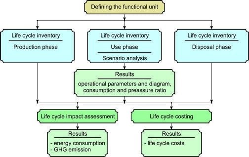
2.1. Methodology of LCA for Pumps/Motors WDS

The LCC analysis of the frequency-controlled pumps/motors in a WDS is based on a model that includes several costs “groups” that can be broken down into three parts: production, use, and disposal. The presented formula, developed by [17] was used to define the new model:
L C C = C i c + C i n Production + C e + C o + C m + C s Use + C e n v + C d Disposal
where Cic are initial costs, purchase price (pump, pipes, auxiliary services); Cin is installation and commissioning costs (including training); Ce are energy costs (predicted cost for system operation, including pump driver, controls, and any auxiliary services); Co are operation costs (labor cost of regular system supervision); Cm are maintenance and repair costs (routine and predicted repairs); Cs are downtime costs (loss of production); Cenv are environmental costs (contamination from pumped liquid and auxiliary equipment); Cd is decommissioning/disposal costs (including restoration of the local environment and disposal of auxiliary services). All parameters in formula (1) are expressed in (€).
The level of sustainability of a WDS is obtained when observing the total value of the LCC calculated in (€), the total amount of consumed energy, measured in (MWh), and the GHG gas emissions calculated in (t-CO2-eq) as a consequence of energy consumption.
From the formula (1), the authors have defined the LCA model, which shows the three boundary stages in the lifecycle of a PU in a WDS system—Figure 2, where input and output elements are energy and CO2 gas emissions.
From this formula (1), other formulas for the total necessary (consumed) energy and gas emission for the production, operation, and disposal of the PU have been derived. Thus, the new formula for the total energy consumption will be as follows:
E t o t = E i c + E i n + E e + E o + E m + E s + E e n v + E d
New formula for total GHG emissions is:
G t o t = G i c + G i n + G e + G o + G m + G s + G e n v + G d
where parameters related to the specific consumption of energy per stage of the lifecycle of PU are expressed in (kWh), while the GHG emissions are expressed in (kg-CO2-eq).

2.1.1. Production Stage

The production process of a specific component (pump, motor, frequency controller) implies the consumption of adequate material assets for production, expressed through capital expenditure and GHG emissions.
Accordingly, formulas have been created, and the defined LCA model was used to calculate the coefficient values for energy consumption in PU production and at the same time, the coefficients values related to GHG emissions during production.
The formulas for energy consumption and GHG emissions are calculated using (5):
E p r o d = E i c + E i n = ( k p r o d ,   p u m p W i c ,   p u m p + k p r o d .   m o t o r W i c ,   m o t o r + k p r o d .   V F D W i c ,   V F D ) + E i n
G p r o d = G i c + G i n = ( g p r o d ,   p u m p W i c ,   p u m p + g p r o d .   m o t o r W i c ,   m o t o r + g p r o d .   V F D W i c ,   V F D ) + G i n
where kprod, index stands for the factor of energy consumption per unit (kWh/kg); gprod, index represents the factor of GHG emissions (kg-CO2-eq./kg); and Wic, index is the weight ratio of the material (steel, copper, aluminum, paint...) in a component (kg). Energy consumption and GHG emissions factors relate only to the production process of the materials themselves and their processing to obtain a certain component. The Ein and Gin parameters define the energy consumption and GHG emissions during the installing, testing, and transporting the pump, electric motor, and VFD, which, however, will not be dealt with in this section.

2.1.2. Use Stage

During the exploitation, for each of the components of a PU, working parameters are defined for WDS. In addition to their operation, the following essential parameters, related to the pump/motor drive unit, are also monitored:
C u s e = C e + C o + C m + C s
where: Ce stands for the energy consumption of the electric motors of the pumps as well as other components in the system, such as the frequency controller. Energy consumption is predominant in LCC calculation, especially if the pumps are performing over 2000 operating hours on average on an annual basis. Co stands for the costs related to pump system management (i.e., PU monitoring). In the operation of nonautomated systems, it is necessary to engage workers to monitor PU performance and to perform corrections in the system operation. In fully automated systems, this parameter can be reduced according to daily needs. Also, it can be reduced by a number of system adjustments to a certain period (once a year, twice a year, or more years), depending on the use of PU in WDS. Cm is a parameter related to PU maintenance and servicing. Servicing can be scheduled according to the number of operating hours of the drive unit or according to the monitoring, such as vibration diagnostics. However, it has been proven in practice that servicing intervals are impacted by various factors such as load variation (flow—Q, pressure—p, and revolution per minute—n), the number of start-ups and shutdowns, and other factors related to working fluid (water purity and temperature). The maintenance can be planned depending on the ability to monitor operating parameters and pump/motor vibration. Cs is a parameter related to the occurrence of losses within a WDS when the system is not working. Fundamentally, WDS systems are always designed with at least one spare parallel pump in the system, which can replace one system failure. The initial investment is somewhat higher, but the cost of unplanned maintenance is reduced to the repair costs of the pump that failed, without the occurrence of any production losses. The costs related to production losses depend on the downtime interval and depend on a specific case and WDS. All parameters related to Cuse calculation are expressed in (€).
A new formula has been derived from formula (6), which specifies in more detail specific actions related to the calculation of energy consumption and GHG emissions during the use of PU and VFD.
E u s e = ( E e , m o t o r + E e , V F D + e w ( ( f t e s t c t e s t ) + ( f m a i n ,   p u m p c m a i n ,   p u m p ) + ( f m a i n ,   m o t o r c m a i n ,   m o t o r ) + c o v e r h a u l N o v e r h a u l ) ) T
G u s e = ( G e , m o t o r + G e , V F D + g w ( ( f t e s t c t e s t ) + ( f m a i n ,   p u m p c m a i n ,   p u m p ) + ( f m a i n ,   m o t o r c m a i n ,   m o t o r ) + c o v e r h a u l N o v e r h a u l ) ) T
where Ee,index stands for the energy consumption during operation motor+VFD (MWh/year(s)); Ge,index stands for the GHG emissions during operation motor+VFD (kg-eq-CO2/year(s)); ew stands for the work-energy conversion factor (kWh/€); gw represents the work-GHG emissions conversion factor (kg-CO2-eq); ctest is the pump/motor test cost rate (€/test); cmain,index stands for the pump/motor maintenance cost rate (€/h); ftest stands for the number of tests per year (test/year); fmain,index stands for the number of hours per year on maintenance of the pump/motor (h/year); coverhaul stands for the overhaul cost rate (€); Noverhaul stands for the number of overhauls during the planning period (-); and T is the planning period (year(s)).

2.1.3. Disposal Stage

In the end-of-life process of WDS components such as PU and VFD, only the recycling process is considered, since the mentioned components have no significant impact on the environment, except for the recycling process.
According to the LCC formula, where the environmental impact costs are neglected, and only the recycling process costs are included in the calculation, the disposal costs can be calculated as follows:
C e o l ,   d i s p = C e n v + C d = C d
Formulas for energy consumption and GHG emissions during recycling are the following:
E e o l ,   d i s p = e r e c W t m m
G e o l ,   d i s p = g r e c W t m m
where erec stands for the recycling-energy conversion factor (kWh/kg); grec stands for the GHG emissions-energy conversion factor (kg-CO2-eq/kg), and Wtmm stands for the total mass of the materials (cast iron, steel, copper, aluminum, PVC, bronze, etc.) in (kg).

2.2. Functional Unit

The functional unit for a WDS is the total volume of water pumped during one year, measured in (m3). The main task of WDS is to deliver a sufficient amount of drinking water over a given time interval. The total volume of water distributed (m3) on a daily, monthly, or annual basis typically varies due to weather and time of the year (summer–winter), or due to a consumption resulting from increased activities in industry or agriculture or other factors (holidays, etc.). Typical values in water consumption are usually the average values. The maximum consumption value can be determined by adding 10%–30% [18] of an average observed consumption (on a daily, monthly, or annual basis) or the measured current consumption. Depending on the WDS type (branched- or grid-type network configuration) it is necessary to determine peak loads. The most precise data on any process including the distributed quantity of water can be obtained when the existing system is equipped with monitoring and data acquisition devices [19]. By measuring the volumes of water being distributed as well as the pressures, the data are gathered allowing the analysts and engineers to adequately respond and adjust the current WDSs’ PU, to achieve a more efficient system and lower energy consumption. In order to prevent variations in the distributed water volumes during a given period, it is necessary to provide the possibility of optimization and correction of PU during the lifecycle of WDSs’ PU in frequency-controlled systems.
In order to determine the pump/motor performance in a WDS, three fundamental indicators should be used: pump head, system pressure, and the number of operating PU’s. According to these values, the diagram of the parallel operating pumps will be drawn for two basic scenarios.

2.3. Energy Consumption in the Use Stage—Ee

Pump and motor energy consumption data are essential for defining the best ratio of the drive unit fuel consumption (kWh) and the amount of produced water that is pumped into the WDS by the frequency-controlled pumps. The optimization period of the PU is set daily. The number of pumps to be used for a particular WDS is calculated according to the real daily consumption period and the average consumption on a monthly and annual basis for other exploitation variants of frequency-controlled motors in a WDS. Also, a 24 h time interval is used to calculate the costs of consumed electrical energy because the pumps are set to operate during that time interval. What matters most in a WDS is establishing a balance between the costs of production and the quality of drinking water distribution. In the energy consumption model for a real PU, the consumption of electricity based on the two-tariff options of the electricity pricing is included when an electricity distribution system provides lower and higher tariffs of electrical energy (electricity generated mainly with dirty technologies), as well as in the second case, the consumption of electricity generated by various production systems (so-called “green” energy generated by wind generators, solar energy, photo panels, etc.). When it comes to an electricity distribution system that has an average tariff for electrical energy during the entire day, the formula is simplified and takes into account only the single electricity tariff.
The cost of energy consumed during 24 h based on two-tariff options can be represented by the following formula:
C e = S P n i = 1 j E n [ P C ( i , j ) ] + S P d k = j + 1 l E d [ P C ( k , l ) ]
where the SPn stands for the night tariff in (€/kWh), i stands for the start of the night tariff interval (h), j stands for the end of the night tariff interval (h), PC (i, j) stands for the number of (combinations) of the pumps in operation during the night mode, SPd stands for the day tariff (€/kWh), k stands for the start of the day tariff interval (h), l stands for the end of the day tariff interval (h), PC(k,l) stands for the number of (combinations) of the pumps in operation during the day mode, En and Ed stand for the consumed electricity during the night/day operation mode of pumps/motors (kWh). Time intervals can be defined depending on the power of the electric motor drive and the pump capacity affecting the speed of electric energy withdrawal from the electricity grid. Parameter E can be calculated as the product of the multiplication of the flow and the pressure supplied by one pump with the inclusion of appropriate pump and motor efficiency coefficients. Therefore, current energy consumption on an hourly basis can be calculated as follows:
E = t = 1 n P ( t ) η ( t ) t o t Δ t = t = 1 n γ Q ( t ) H ( t ) η ( t ) p u m p η ( t ) m o t o r Δ t 60 3600
where t stands for the number of pump/motor operation cycles during one day; P(t) stands for the pump drive energy (kW); γ stands for the water density (N/m3); Q(t) stands for the pump flow rate (m3/s); H(t) stands for the pump head (m); η ( t ) t o t = η ( t ) p u m p × η ( t ) m o t o r stands for the total efficiency, pump efficiency, and motor efficiency; Δt stands for the time interval of the pump/motor operation, expressed in (min). Formula (13) can be used for a pump operating within the system of either different or the same pump volumes. It should be noted that the frequency-controlled motors of each of the WDS pumps are adjusted to work under the same revolutions per minute in the modes with two or more parallel operating pumps in a WDS.
Daily consumption diagrams are particularly important when designing primary and secondary water supply networks, especially the pump stations and tank facilities. In such WDSs, the shortest water consumption cycle is expressed as one day when the consumption is at the peak during the year, which implies the synchronization of components operation in a WDS (pump stations and tanks) with similar supply conditions occurring every 24 h.
Water demand (consumption) patterns are usually obtained through monitoring at delivery locations (critical points in the network, the pressure of the amplification station, tanks, control points with permanent or mobile equipment). In this way, actual consumption data are obtained, because this approach allows separation of various consumptions, while on the other side, excludes the losses caused by leakage.
For WDS water supply, an energy equation can be used for calculating the pump head, starting from the water level in the source (pump tank), through any pump “i”, up to the pump station outlet:
H p i = ( H o u t H s o u r c e ) + Δ h p i + Δ h s ( j ) i + Δ h m ( i , j ) = ( H o u t H s o u r s ) + Δ h ( j ) i = H c ( j ) i
where H p i stands for the pump head “i” (m); H o u t stands for the piezometric height at the output of the pump station (m); H s o u r c e stands for the water level at the source (m); Δ h p i   are losses in the pump “i” pipeline (depends on the characteristics of the suction and displacement pump pipework and the flow through the pump); Δ h s ( j ) i are losses in the collector pipe for the pump “i” (depends on the characteristics of the collector pipe, the number and arrangement of the pump “j” in parallel operation with pump “i”, and of all the flow of active pumps); Δ h m ( i , j ) are losses in the main (pressure) pipeline (depend on the characteristics of the main pipeline and the total flow of all the pumps currently in operation); Δ h ( j ) i are total pump losses “i” in parallel operation with pumps “j” from suction ring pump to outlet from pump station; H c ( j ) i stands for the pipeline characteristics for the pump “i” from the water level of the wall and fill to the output from the pump station.

3. Results

The developed LCA/LCC model for evaluation of WDS was tested in Novi Sads’ WDS. This WDS consists of five identical pumps, connected in parallel to the main pipeline for distribution of drinking water for the city of Novi Sad (approximate population of 300,000). The pumps were installed in the WDS in 2009, and by 2018 there was one overhaul on each electric motor when the bearings were replaced (the overhauls were performed when needed, i.e., at the time when the damage occurred, the pump was stopped and the overhaul was done). The pumps were initially coated on the inside with an epoxy coating, and the pump impellers were made of stainless steel to prevent corrosion. By 2018, the pumps had performed on average 35,000 working hours. The performance of the pumps over the observed 12 month period (July 2017 to June 2018) is shown in Figure 3, wherein the observed year, the pumps performed on average 51.12% of the total time in the year, representing about 4478 (h/year) or 187 (day/year) per pump.
In order to calculate the energy consumption of the PU, measurements of the amount of water distributed under a certain pressure at the pump outlet were monitored, because it is the actual quantity of water that the pump supplies to the system, not including either detailed network losses or the extent of the network friction, which were disregarded, because in further analysis the same network is observed with different usage scenarios for frequency-controlled pumps in the WDS. The measured values will be used to determine the operating capacity of the pump and the power of the motor (i.e., the daily and total energy consumption over the observed period). It needs to be emphasized that in the WDS, the maximum of four pumps are operating during the water consumption peaks, while the fifth one serves as a spare. The simulation of demanded consumption and provision of the minimum working pressure was done in the EPANET program [20], according to which the necessary operating parameters (pressure and average flow rate) were determined. The advantage of Novi Sads’ WDS is that by using the frequency-controlled pumps connected in parallel, it is possible to adjust the flow, or current water consumption during the day, as well as the pressures that can be adjusted by the frequency change in the electric motor. Contrary to the study [15], where the observed pump has approximately constant values of the operating point, the operating point of Novi Sads’ WDS changes during the day depending on whether two, three, or four pumps operate in the system.
The fifth pump is a spare, and the combination of the pumps provides an approximate number of operating hours during the year (Figure 3.). In October, the overhaul of the bearings on the electric drive motor of P2 was performed, and it was the last pump to sustain bearing replacement (Figure 3.). Bearings of the electric motors operated for about 30,000 work hours on average, which is considerably below the designed 100,000 h.

3.1. Characteristics of PU in the Pump Station

The parameters describing the characteristics of the PU are shown in Table 1. The designed pump head values and the values of the power required for the pump drive were used to determine and model the curves and to obtain the operating points of the use of two, three, and the maximum of four pumps in parallel operation, as shown in Figure 4 and Figure 5.
According to the formula (14), all the functional flow-dependent losses were calculated Δ h p i ; Δ h s ( j ) i ; Δ h m ( i , j ) and Δ h ( j ) i , using the references [22,23].
Based on the coefficients of local resistances in the suction and discharge pipelines and the flow through the pump “i”, the following loss values were obtained:
Δ h p 1 , 5 = 8 Q 2 g π 2 d u 4 ξ u + 8 Q 2 g π 2 d p 4 ξ p = 9.43 Q 2 = b p 1 , 5 Q 2
where du is the diameter of the suction pipeline (value 0.5 m); dp is the diameter of the pressure pipeline (value 0.35 m); ξu is the total coefficient of local resistance of the suction pipelines of the pumps; ξp is the total coefficient of local resistance of the pressure pipelines of the pumps; pumps P1 and P5 were defined as the most critical pumps in terms of the length of the pipeline, which is why the loss in pipelines P1 and P5 are equal and expressed as a loss coefficient b p 1 , 5 = 9.43 . For the flow value Q = 400 L/s, total resistance coefficients are ξu = 0.55, i ξp = 1.58.
Local resistance losses of the discharge pump station pipeline were calculated according to the following formula:
Δ h m ( i , j ) = 8 Q ( i , j ) 2 g π 2 d p r e s 4 ξ m = 0.244 Q ( i , j ) 2 = b m ( i , j ) Q ( i , j ) 2
where dpres stands for the diameter of the pressure pipeline pump station (value 0.9 m); ξm stands for the total coefficient of local resistance of the pressure in pump station pipeline; Q(i,j) stands for the total flow generated by the pumps “i” and “j”, which are currently in operation; b m ( i , j )   stands for the coefficient of losses and amounts b m ( i , j ) = 0.244 .
Coefficients of local resistances in the collection pipeline were calculated for the following pump combinations:
(a)
P1 pump is in parallel operation with P2, P3, and P5 pumps:
Δ h s ( 2 , 3 , 5 ) 1 = 8 Q 2 g π 2 d s 1 4 ξ s 1 + 8 ( 2 Q ) 2 g π 2 d s 2 4 ξ s 2 + 8 ( 3 Q ) 2 g π 2 d s 3 4 ξ s 3 + 8 ( 3 Q ) 2 g π 2 d s 5 4 ξ s 5 = 1.82 Q 2 = b s ( 2 , 3 , 5 ) 1 Q 2
(b)
P5 pump is in parallel operation with P1, P2, and P3 pumps:
Δ h s ( 1 , 2 , 3 ) 5 = 8 Q 2 g π 2 d s 5 ´ 4 ξ s 5 ´ = 0.4 Q 2 = b s ( 1 , 2 , 3 ) 5 Q 2
(c)
Finally, when P5 pump is operating independently, the loss is calculated according to the following formula:
Δ h s ( ) 5 = 8 Q 2 g π 2 d s 5 ´ 4 ξ s 5 ¨ = 1.45 Q 2 = b s ( ) 5 Q 2
where d s 1 ,   d s 2 ,   d s 3 ,   d s 5 ,   d s 5 ´ are diameters of collecting pipelines; ξ s 1 ,   ξ s 2 ,   ξ s 3 ,   ξ s 4 ,   ξ s 5 ´ ,   ξ s 5 ¨ , are the total coefficients of local resistance of the collecting pipelines; ds1 = 0.45 m; ds2 = 0.6 m; ds3 = 0.7 m; ds5 = 0.8 m; d s 5 ´ = 0.5 m; i ξs1 = 0.19; ξs2 = 0.37; ξs3 = 0.033; ξs5 = 0.235; ξ s 5 ´ = 0.3; ξ s 5 ¨ = 1.1.
According to formulas (15)–(18), from the pump inlet to the outlet of the pump station in the pump flow function, and related to pumps P1 and P5 when operating in parallel with pumps P2 and P3, total losses were calculated as follows:
Δ h ( 2 , 3 , 5 ) 1 = b p 1 Q 2 + b s ( 2 , 3 , 5 ) 1 Q 2 + b m ( 1 , 2 , 3 , 5 ) ( 4 Q ) 2 = ( 9.43 + 1.82 + 3.9 ) Q 2 = 15.15 Q 2
Δ h ( 1 , 2 , 3 ) 5 = b p 5 Q 2 + b s ( 1 , 2 , 3 ) 5 Q 2 + b m ( 1 , 2 , 3 , 5 ) ( 4 Q ) 2 = ( 9.43 + 0.4 + 3.9 ) Q 2 = 13.73 Q 2
For the pump flow of Q = 400 L/s per pump, the losses obtained according to (20) and (21) were 2.42 m and 2.2 m. Since the selected pumps achieved 58 m head with the given flow, the difference between these losses was negligible (only 0.22 m) so it was not included in further analysis. Total losses in the pump flow function, for any pump in parallel operation with three other pumps, were calculated on the basis of the mean value:
Δ h ( + 3 ) i = ( 15.15 + 13.73 ) 2 Q 2 = 14.44 Q 2
In case of single-pump operation, the maximum flow that can be reached by one pump is considered to be the maximum flow generated by pump P5. Therefore, for the modelling of any single-pump operation, the P5 pump losses will be used, and its formula, based on (15), (16), and (19), will be as follows:
Δ h ( ) 5 = b p 5 Q 2 + b s ( ) 5 Q 2 + b m ( 5 ) Q 2 = ( 9.43 + 1.45 + 0.244 ) Q 2 = 11.12 Q 2
According to formulas (14), (22), and (23), the diagram of pumps exploitation was drawn for one, two, three, or maximum four pumps in parallel operation; for two exploitation variants:
(a)
the pumps in the pump station maintain constant pressure at the outlet from the pump station and allow tank filling at a certain height point;
(b)
the pumps in the pump station maintain constant pressure on the outskirts of the urban area with a minimum set pressure of 3.5 bar.

3.1.1. Pump Exploitation—Option “a”

Figure 4 shows possible working points of the pumps when the pump station operates in the set pressure maintenance mode at the pump station outlet, which enables the tank filling at the piezo metric height of H o u t 1 = 132   m , and the suction level of the pump is at the minimum height of H s o u r c e 1 = 76.2   m or H s t a t i c 1 = H o u t 1 H s o u r c e 1 .
Based on formulas (14) and (17), the characteristic of the pipeline H c ( + 3 ) i is modeled, which indicates the operation of four pumps in parallel operation is as follows:
H c ( + 3 ) i = H s t a t i c 1 + 14.44 Q 2
Figure 4 also marks H c ( ) i characteristic of the pipeline when one pump is in operation and the pump station level is maximum at the level H s o u r c e 2 = 80.2   m , and the piezo metric height at the outlet is maintained at the level of H o u t 2 = 128   m ; where H s t a t i c 2 = H o u t 2 H s o u r c e 2 .
H c ( ) i = H s t a t i c   2 + 11.12 Q 2
Numbers in Figure 4 indicate possible operating modes of frequency-controlled pumps in different pump operation combinations: point 1—parallel operation of four pumps with Hstatic1; point 2—parallel operation of four pumps at n ≈ 0.91no, operation of the pumps with minimum flow; point 3—one pump in operation at n = 0.85no and with Hstatic2; points 4, 5, 6, and 7 represent the pump operation combinations with different piezometric heights of pump suction in the pump station and outlet pressure from the pump station towards the tank.
The framed area a-b-c-d in Figure 4 provides a safe filling level of 50.5 m high-pressure tank under all possible regular WDS operating conditions. The number of pumps turned on/off is defined on the basis of the number of revolutions per minute and the minimum allowed flow of the pump, which is defined by the operating frequency of the electric motor, pressure at the reference point in the city, and level meters in the tank of the source and the elevated tank.

3.1.2. Pump Exploitation—Option “b”

Under conditions when the pump station is operated according to the pressure in the reference node on the outskirts of the urban area, the pressure at the outlet from the pump station will not be constant and will vary depending on the current flow or consumption. In other words, the value of Hout in Equation (14) is not constant and varies with the flow.
The dependence of Hout(Q) is determined indirectly based on the data obtained from simulations on the WDS hydraulic model. For this purpose, the diagrams of pump station flow and pressure at node 94 were used in conditions when the piezometric height at the outlet of the pump station is maintained at 120 m a.s.l—Figure 6a and 128 m a.s.l—Figure 6b.
Under condition when the pressure at node 94, on the periphery of the city, is constant and equals 35 m, and based on the consumption diagram, Table 2 was created, showing the values of the Hout(Q) of the pump station depending on the flow performed by the pump station.
Based on the data from Table 2, the curve Equation (26) shows the dependence of piezometric heights on the flow (obtained by the method of least squares), which connects the obtained operating points.
H o u t ( Q ) = 115.0618 + 2.6528 Q + 3.2518 Q 2
By replacing formula (26) with the energy Equation (14), taking into account losses (22) and (23), the following characteristics of the pipeline are obtained from the water level in the pump station (source) to the pump station outlet, under conditions when the pump station with four pumps is in operation and when only one pump is operating:
H c ( + 3 ) i = [ H o u t ( 4 Q ) H s o u r s 1 ] + 14.44 Q 2
H c ( ) i = [ H o u t ( Q ) H s o u r s 2 ] + 11.12 Q 2
By the linear interpolation of the calculation of losses for the cases when either three or two pumps are operating, the following formulas are obtained:
H c ( + 2 ) i = [ H o u t ( 3 Q ) H s o u r s 1 , 2 ] + 13.33 Q 2
H c ( + 1 ) i = [ H o u t ( 2 Q ) H s o u r s 1 , 2 ] + 12.23 Q 2
By using Equations (26)–(30), in Figure 5 the operating points of the pumps have been considered when the pump station operates in the set pressure maintenance mode on the periphery of the urban area (node 94).
Characteristics of the pipeline (Figure 5) are indicated with H c ( + 3 ) i (Hsours1 = 76.2 m), when four pumps are in operation and the water level in the pump station is Hsours1 = 76.2 m (minimum possible level). The characteristics of the pipeline when three, two, and one pump is in operation at the same water level in the pump station are indicated with dashed lines.
H c ( ) i (Hsours2 = 80.2 m) indicates the pipeline characteristics when one pump is in operation and the water level in the pump station is Hsours2 = 80.2 m (maximum possible level). The dot dash lines indicate the pipeline characteristics when two, three, and four pumps are in operation at the same level of water in the pump station (Figure 5).
Since, according to the design, the pumps in the pump station operate under the frequency-controlled revolution per minute in all pumps, the highlighted area in Figure 5, limited by the curve H c ( ) i (Hsours2 = 80.2 m), H−Q pump characteristic at no, the curve H c ( + 3 ) i (Hsours1 = 76.2 m), the line a-b-2, and the vertical Q = 180 L/s; represents the area of possible operation modes of the pumps. The line a-b-2 has not been defined in advance, and its position depends on the method of selection of minimum flows for two, three, and four pumps in parallel operation. In this example of VFD pump/motor application, the number of pumps in operation is defined by measuring the revolution per minute and the minimum flow that pumps are allowed to reach, which are defined on the basis of the operating frequency of the electric motor, the pressure at the reference point in the city, and the level meter in the source tank.

3.2. Planned and Actual Water Consumption in the WDS

One-hour water consumption recording is commonly accepted and mostly used in practice. The maximum consumption recorded in that time period is most often represented as hourly (or daily) consumption peak, as shown in Figure 7, of water for a city having a population of 300,000 consumers, which also represents the day with the highest consumption in the observed 2017/2018.
In Figure 7, the demand for larger quantities of water can be noticed from 6:00 a.m. until 11:00 p.m. By calculating the mean values on an annual basis, the water consumption is obtained at the level of 1075 L/s. Figure 8 shows the maximum daily consumption for the observed 2017/2018, which will also be the basis for the operation of the PU, according to option “a” and option “b” for WDS.
Regarding the diagram in Figure 8, electrical energy consumption for the pumps in parallel operation was calculated depending on the daily water consumption. Figure 9 and Figure 10 show the consumption of electrical energy for the pumps in combinations of two, three, and four pumps on a daily basis, as well as the consumption of electrical energy of one pump when the system operates according to the parameters of the options “a” and “b”.
In the presented research, the pump station optimization was not performed. However, the calculations suggest possible variant solutions that can make significant savings in electrical energy consumption as well as GHG emissions, which the results will show.

3.3. LCA/LCC Coefficients

In order to carry out the assessment of the lifecycle of a product LCA—which, in this case is a pump, a motor, and a VFD—formulas (4), (5), (7), (8), (12), and (13) of the operation model are used, using the coefficients shown in Table 3, Table 4 and Table 5. The coefficients have been calculated for LCA values per one PU (motor, pump, VFD), while the testing and reparation coefficients have been selected on the once-in-ten-years basis and the planned exploitation period of 40 years.
Factors kprod, index and gprod, index have been obtained on the basis of lifecycle inventory (LCI) analysis of the amount of consumed energy and GHG emissions for the production of each of the components. Table 4 shows the values of material quantities required for the pump, motor, and VFD, the amount of the consumed energy, and the coefficient of production, obtained as the quotient of total consumed energy for the material production and the total mass of the component. The EcoInvent 3 LCI database was used for the processes listed in Table 4.
Table 5 shows the parameters for the calculation of electrical energy consumption and GHG emissions when one pump/motor/VFD is operating. To calculate the displayed parameters, the data obtained from the testing and repairing of the pumps/motors were used. The operation and energy conversion factors ew were obtained on the basis of the price of consumed kWh per monetary unit and refer to both the energy prices in the observed environment and the global energy prices 0.13 €/kWh for 2017/2018. This parameter has variable value and can be adjusted to the current electrical energy price. The loss-related parameters Cs are not included because in the given example, the losses can be avoided by an additional pump that replaces any failed pump and provides a higher reliability of the WDS.
Table 6 shows the parameters related to the recycling of PU and VFD, using the data obtained from the software (EcoInvent 3 LCI database) and a procedure similar to the one shown in Table 4. All the factors (energy and GHG emissions) are related to the mass recycling of certain materials (copper, steel, cast iron, PVC, etc.) of which components are made.
Factors erec and grec show that recycling the reusable materials reduces both the energy consumption and GHG emissions.

4. Discussion

The results obtained in this research include several scenarios for the use of a PU which, according to the diagram in Figure 3, operates on average 187 days a year. The PU operates in two different modes when the frequency adjusts to the current water consumption in the system (Figure 10)—scenario 1, and when the pump operates in a relatively balanced mode when it supplies the water tank that provides a smaller volume of water for consumption (Figure 9)—scenario 2. Both scenarios imply two-tariff options of the electricity pricing at prices that are valid in Serbia, burning of fossil fuels and the use of Serbia’s hydropower, with the cheaper night tariff of electrical energy. Scenarios 3 and 4 imply the operation of both systems, but with prices that apply in Germany, as the country with the most expensive price of electrical energy, which is equal for both night and day tariffs, amounting to 0.15 €/kWh [25]. Scenarios 5 and 6 include the modes of operation when energy from the “green” sources (wind generators, solar cells...) is consumed, or when the electricity is cheaper in the daily operation mode compared with the electricity generated for the night operation mode (without changing operation modes and pump combinations)—the example of Spain, where the price of electrical energy in 2017 was 0.1 €/kWh [26]. Table 7 shows the data related to LCC, consumed energy, and GHG emissions in each of the scenarios obtained by formulas 10 and 11 for the operation of one pump, 187 h/year at 40 year exploitation period.
In Figure 11a, the scenario 1 shows energy consumption of the PU in operation according to the parameters of the flow measurement at the outlet from the pump station and the pressure measurement at the node in the city. Based on the presented values, it can be noticed that energy consumption is significantly smaller in relation to the scenario 2, which exceeds scenario 1 by all parameters (GHG and costs). However, scenario 2 allows for the supply of sufficient quantity of drinking water during the day, in case of a stoppage or failure and does not significantly affect the operating parameters of the system. Scenario 2 provides better distribution of water in the system with a minimum reserve compared with scenario 1.
However, the disadvantage of scenario 2 is that the water level should be raised to higher values, and thus more energy is consumed and more GHG is emitted. The other four scenarios are similar regarding the operation, but for different areas (scenario 3 and 4 for Germany, scenario 5 and 6 for Spain).
Based on the results shown in Figure 11a,b, the following facts can be determined: the PU supplying WDS in Serbia produces the highest amount of GHG emissions per spent monetary unit (€)—Table 7. Compared with Germany, which has one of the highest prices of electrical energy in the EU, this ratio is 2.41 (ratio 5.85/2.41, Serbia/Germany) times higher compared with Spain 2.8 (ratio 5.85/2.09, Serbia/Spain), the ratio of scenarios 1, 3, and 5 in Figure 11b, Table 7. Regarding scenario 2, the amount of GHG emissions per monetary unit is even higher and ranges from 2.54 (ratio 6.61/2.60, Serbia/Germany) to 2.95 (ratio 6.61/2.24, Serbia/Spain), the ratio of scenarios 2, 4, and 6 in Figure 11 b, Table 7. Regardless of the fact that Serbia consumes the least amount of money for the same amount of consumed energy and produced water, in comparison with Germany and Spain, which in their energy production use the so-called “green energy”, Serbia produces from 2.41 to 2.8 times (with pump operation option “b”) and from 2.54 to 2.95 times (with pump operation option “a”) higher amount of GHG per monetary unit. Analyzing the amount of tons of GHG emissions, Serbia emits from 1.61 (ratio 1018.18/630.24, Serbia/Germany) to 2.19 (ratio 1018.18/463.13, Serbia/Spain) times higher amount of GHG in tons. The results show that the amount of consumed energy normally affects the GHG emissions, but the amount of GHG emissions depends on the source of the obtained energy for driving the PU in the WDS. Since production costs are related only to the operation of one pump, it is not difficult to calculate the costs and GHG emissions for the combined operation of two, three, and four pumps. Normally, the variability in costs and GHG emissions is influenced by the main functional unit—flow, which is variable on both the daily and annual basis. This results in the variability of other parameters and directly depends on water consumption.
End of life for water PU considers recycling process where materials such as steel, aluminium, copper, and other are recovered, and this lowers costs, energy, and GHG emission (Table 6). This positive effect on cost, energy, and GHG emission is reflected through factors erec and grec (i.e., their negative values).

5. Conclusions

Presented in this study is the LCA/LCC model for assessing the costs, energy consumption, and GHG emissions during the PU lifecycle in WDS. Based on this research, it can be concluded that Serbia consumes the least amount of money for the same amount of consumed energy and produced water, in comparison with Germany and Spain, which in their energy production use the so-called “green energy”. Also, Serbia produces a higher amount of GHG per monetary unit (€). By using “green energy”, GHG emissions can be significantly reduced, especially when Serbia is concerned, because it generates a considerably higher amount of energy from thermal power plants. The results presented in this paper show that the EU countries with notably higher prices of electrical energy also have a few times lower GHG emissions. Investment in alternative energy sources will increase the price of electrical energy, but will also significantly reduce GHG emissions.
The developed LCA/LCC model for evaluation of PU can be implemented to any PUs in the WDS system with necessary modification of input values for each of the components of PU and using EcoInvent 3 LCI database. Future research will be focused on PU optimization and their operation in the current WDS supply and the monitoring of the possible reduction of PU efficiency through more prolonged exploitation.

Author Contributions

The contribution of the authors to this manuscript can be defined as conceptualization, M.J., and G.O.; methodology, M.J. and V.K.; software, B.A. and M.I.M.; validation, M.J. and M.O.; formal analysis, M.J.; investigation, M.O.; resources, V.K.; data curation, S.S.; writing—original draft preparation, M.J.; writing—review and editing, S.S.; visualization, B.A. and G.O.; supervision, S.S.; project administration, M.J.

Funding

This research was partially funded by Ministry of Education, Science and Technology Development of the Republic of Serbia under the Grant 401-00-00589/2018-09.

Conflicts of Interest

The authors declare no conflict of interest.

References

  1. Ferreira, F.J.; Fong, J.A.; Almeida, A.T. Ecoanalysis of Variable-Speed Drives for Flow Regulation in Pumping Systems. IEEE Trans. Ind. Electron. 2011, 58, 2117–2125. [Google Scholar] [CrossRef]
  2. Burton, F.L.; Stern, F. Water and Wastewater Industries: Characteristics and DSM Opportunities; U.S. Department of Energy Office of Scientific and Technical Information: Washington, DC, USA, 1993.
  3. Tegeltija, S.; Lazarevic, M.; Stankovski, S.; Cosic, I.; Todorovic, V.; Ostojic, G. Heating circulation pump disassembly process improved with augmented reality. Therm. Sci. 2016, 20, S611–S622. [Google Scholar] [CrossRef]
  4. Cabrera, E.; Cobacho, R.; Pardo, M.A. Energy Audit of Water Networks. J. Water Resour. Plan. Manag. 2010, 136, 669–677. [Google Scholar] [CrossRef]
  5. Stjepanovic, A.; Stojcic, M.; Stjepanovic, S. Hybrid Power Energy Source Based on Pem Fuel Cell/Solar System. J. Mechatron. Autom. Identif. Technol. 2019, 4, 5–8. [Google Scholar]
  6. Loss, A.; Toniolo, S.; Mazzi, A.; Manzardo, A.; Scipioni, A. LCA comparison of traditional open cut and pipe bursting systems for relining water pipelines. Resour. Conserv. Recycl. 2018, 128, 458–469. [Google Scholar] [CrossRef]
  7. Uche, J.; Martínez-Gracia, A.; Círez, F.; Carmona, U. Environmental impact of water supply and water use in a Mediterranean water stressed region. J. Clean. Prod. 2015, 88, 196–204. [Google Scholar] [CrossRef]
  8. Fantin, V.; Scalbi, S.; Ottaviano, G.; Masoni, P. A method for improving reliability and relevance of LCA reviews: The case of life-cycle greenhouse gas emissions of tap and bottled water. Sci. Total Environ. 2014, 476–477, 228–241. [Google Scholar] [CrossRef] [PubMed]
  9. Chang, Y.; Choi, G.; Kim, J.; Byeon, S. Energy Cost Optimization for Water Distribution Networks Using Demand Pattern and Storage Facilities. Sustainability 2018, 10, 1118. [Google Scholar] [CrossRef]
  10. Herstain, L.; Filion, Y.; Hall, K. Evaluating environmental impact in water distribution system design. J. Infrastruct. Syst. 2009, 15, 241–250. [Google Scholar] [CrossRef]
  11. Wu, W.; Maier, H.; Simpson, A. Multiobjective optimization of water distribution systems accounting for economic cost, hydraulic reliability, and greenhouse gas emissions. Water Resour. Res. 2013, 49, 1211–1225. [Google Scholar] [CrossRef] [Green Version]
  12. Makov, T.; Meylan, G.; Powell, J.; Shepon, A. Better than bottled water?—Energy and climate change impacts of on-the-go drinking water stations. Resour. Conserv. Recycl. 2019, 143, 320–328. [Google Scholar] [CrossRef]
  13. Arden, S.; Ma, X.; Brown, M. Holistic analysis of urban water systems in the Greater Cincinnati region: (2) resource use profiles by emergy accounting approach. Water Res. X 2019, 2, 1000012. [Google Scholar] [CrossRef] [PubMed]
  14. Schaefer, T.; Udenio, M.; Quinn, S.; Fransoo, J.C. Water risk assessment in supply chains. J. Clean. Prod. 2019, 208, 636–648. [Google Scholar] [CrossRef]
  15. Nault, J.; Papa, F. Lifecycle Assessment of a Water Distribution System Pump. J. Water Resour. Plan. Manag. 2015, 141, A4015004. [Google Scholar] [CrossRef]
  16. Filion, Y.R.; MacLean, H.L.; Karney, B.W. Life-Cycle Energy Analysis of a Water Distribution System. J. Infrastruct. Syst. 2014, 10, 120–130. [Google Scholar] [CrossRef]
  17. Hydraulic Institute, Europump and the US Department of Energy’s Office of Industrial Technologies (OIT). Pump Life Cycle Costs: A Guide to LCC Analysis for Pumping Systems. Available online: https://www1.eere.energy.gov/manufacturing/tech_assistance/pdfs/pumplcc_1001.pdf (accessed on 25 January 2019).
  18. Trifunovic, N. Introduction to Urban Water Distribution; Taylor & Francis/Balkema: Leiden, The Netherlands, 2005. [Google Scholar]
  19. Senk, I.; Ostojic, G.; Jovanovic, V.; Tarjan, L.; Stankovski, S. Experiences in developing labs for a supervisory control and data acquisition course for undergraduate mechatronics education. Comput. Appl. Eng. Educ. 2015, 23, 54–62. [Google Scholar] [CrossRef]
  20. EPANET Application for Modeling Drinking Water Distribution Systems. Available online: https://www.epa.gov/water-research/epanet (accessed on 24 February 2019).
  21. Vojvodinaprojekt. Preliminary Design of High Pressure Pump Stations STRAND; Vojvodinaprojekt: Novi Sad, Serbia, 2005. [Google Scholar]
  22. Idelʹchik, I.E.; Fried, E. Handbook of Hydraulic Resistance; Hemisphere Pub. Corp.: Washington, DC, USA, 1986. [Google Scholar]
  23. Hajdin, G. Mechanics of Fluid—Introduction to Hydraulics; Faculty of Civil Engineering: Belgrade, Serbia, 2002. [Google Scholar]
  24. Municipal Water Company project. Determining water consumption; Municipal Water Company: Novi Sad, Serbia, 2017. [Google Scholar]
  25. Statista. Available online: https://www.statista.com/statistics/595803/electricity-industry-price-germany (accessed on 14 January 2019).
  26. Statista. Available online: https://www.statista.com/statistics/595813/electricity-industry-price-spain/ (accessed on 14 January 2019).
Figure 1. LCA/LCC model for evaluation of PU in WDS. PU: pump unit. WDS: water distribution system. GHG: greenhouse gas. VFD: variable frequency drive.
Symmetry 11 01181 g001
Figure 2. PU lifecycle stage in WDS.
Symmetry 11 01181 g002
Figure 3. Percentage of pump operation in the observed year.
Symmetry 11 01181 g003
Figure 4. Pump operation diagram in constant-pressure maintenance mode at the pump station output.
Symmetry 11 01181 g004
Figure 5. Pump operation diagram in constant-pressure maintenance mode at the periphery of the city.
Symmetry 11 01181 g005
Figure 6. Consumption and pressure ratio (simulation in EPANET software [20]): (a) for Hout = 120 m; (b) for Hout = 128 m.
Symmetry 11 01181 g006aSymmetry 11 01181 g006b
Figure 7. Demand pattern in Novi Sad, Serbia [24].
Symmetry 11 01181 g007
Figure 8. The relationship between current demand (option “b”) and reservoir supply (option “a”).
Symmetry 11 01181 g008
Figure 9. Power consumption of the pump(s) according to the option “a”.
Symmetry 11 01181 g009
Figure 10. Power consumption of the pump(s) according to the option “b”.
Symmetry 11 01181 g010
Figure 11. (a) Costs, energy, and GHG emissions for one PU according to the scenario; (b) Emission and cost ratio Gtot1/Ctot1.
Symmetry 11 01181 g011
Table 1. Operating parameters of the Pump, Motor, and VFD [21].
ParameterUnitValue
Rated flow(L/s)450
Rated head(m)52
Rated power—Motor(kW)315
Rated power—VFD(kW)9
Pump Peak efficiency(%)87.5
Motor Peak efficiency(%)96.3
Pump Capital Cost(€/per unit) *50.000
Motor Capital Cost(€/per unit) *40.000
VFD Capital Cost(€/per unit) *28.000
* Without the costs of transportation, installation and testing, or commissioning.
Table 2. The dependence of the piezometer heights at the outlet from the pump station.
Q (L/s)Hout (m a.s.l)Q (L/s)Hout (m a.s.l)Q (L/s)Hout (m a.s.l)Q (L/s)Hout (m a.s.l)
180115.7550117.4950120.51350124.8
250116.0650118.11050121.41450125.9
350116.4750118.81150122.51550126.9
450116.9850119.61250123.51650128.2
* Meters above sea level (m a.s.l.).
Table 3. Conversion factors for the production of components.
ParameterUnitValue
kprod, pump(kWh/kg)3.15
kprod, motor(kWh/kg)2.2
kprod, VFD(kWh/kg)11.3
Wic, pump(kg)1107
Wic, motor(kg)2831
Wic, VFD(kg)62.37
gprod, pump(kg-CO2-eq./kg)2.59
gprod, motor(kg-CO2-eq./kg)2.19
gprod, VFD(kg-CO2-eq./kg)12.85
Table 4. Conversion factors for the production of components obtained by LCI.
LCIValueEnergy for ProductionEmission GHGkprod,indexgprod,index
Pump(kg)(kWh)(kg-CO2-eq)(kWh/kg)(kg-CO2-eq./kg)
market for cast iron production—GLO*6951329.951493.11kprod,pump

3.15
gprod,pump

2.59
market for steel, chromium steel 18/8— GLO*1771526.91835.26
market for metal working, average for chromium steel production— GLO*177483.99339.53
market for bronze— GLO*25103.69153.1
market for silicon carbide— GLO*421.5930.12
market for alkyd paint, white, without solvent, in 60% solution state— GLO*426.1322.63
market for casting, bronze— GLO*254.681.59
Electrical motor(kg)(kWh)(kg-CO2-eq/kg)(kWh/kg)(kg-CO2-eq./kg)
market for metal working, average for steel production— GLO*10552700.212263.294kprod,motor

2.2
gprod,motor

2.19
market for steel, low-alloyed— GLO*10552255.0612108.202
market for cast iron— GLO*441843.90947.431
market for copper— GLO*110227.63558.8027
market for epoxy resin, liquid— GLO*170.32116.254
market for aluminum, cast alloy— GLO*3187.4198.72751
market for wire drawing, copper— GLO*11080.6673.55919
market for alkyd paint, white, without solvent, in 60% solution state— GLO*639.2033.94907
market for polyvinylchloride, bulk polymerized— GLO*60.0913.19395
Variable frequency drive(kg)(kWh)(kg-CO2-eq/kg)(kWh/kg)(kg-CO2-eq./kg)
market for electronics, for control units— GLO*19.845495.13550.2368kprod,VFD

11.3
gprod,VFD

12.85
market for printed wiring board, for power supply unit, desktop computer, Pb containing— GLO*2.835134.97164.7126
market for metal working, average for steel product manufacturing— GLO*14.17536.2830.40966
market for steel, low-alloyed— GLO*14.17530.2928.32584
market for polyvinylchloride, bulk polymerized— GLO*8.5050.1318.70243
market for aluminum, cast alloy— GLO*2.8357.999.02879
* GLO-global, activities which are considered to be an average valid for all countries in the world.
Table 5. Maintenance, Testing, and Repair Parameters.
ParameterUnitValue
ew(kWh/€)7.69
gw(kg-CO2-eq./kWh)1.077/0.665/0.487 *
ftest(test/year)0.1
fmain,pump(h/year)75
fmain,motor(h/year)50
ctest(€/test)1000
cmain,pump(€/h)50
cmain,motor(€/h)50
coverhaul(€)15,000
Noverhaul(-)0.1
T(year(s))40
* The coefficient depends on the price of kWh el. energy in EU countries (Serbia, Germany, and Spain).
Table 6. Conversion factors for product recycling.
ParameterUnitValue
erec(kWh/€)−2.32
grec(kg-CO2-eq./kg)−2.13
Wtmm(kg)2563
Al(kg)33.83
Steel(kg)2382.17
Copper(kg)110
El.scrap(kg)22.68
PVC(kg)14.5
Table 7. Results of costs, energy, and GHG emissions for one pump unit.
ScenarioCtot1
(×103 €)
Ctot40
(×103 €)
Etot1
(MWh)
Etot40
(MWh)
Gtot1
(t-CO2-eq.)
Gtot40
(t-CO2-eq.)
Gtot1/Ctot1
(kg-CO2-eq.)/€
1173.892316.50945.0537,627.401018.1840,555.045.85
2179.162527.021100.4743,844.131185.6947,255.536.61
3241.235010.03945.0537,627.40630.2425,037.502.43
4261.445818.201100.4743,844.13733.6529,173.912.60
5220.554182.73945.0537,627.40463.1318,352.832.09
6240.154966.891100.4743,844.13538.9221,384.692.24

