A Bi–LSTM and k-NN Based Method for Detecting Major Time Zones of Overloaded Vehicles

Abstract

Overloaded vehicles such as large cargo trucks tend to cause large traffic accidents. Such traffic accidents often bring high mortality rates, including injuries and deaths, and cause fatal damage to road structures such as roads and bridges. Therefore, there is a vicious circle in which a lot of the budgets is spent for accident restoration and road maintenance. It is important to control overloaded vehicles that are around roads in urban areas. However, it often takes a lot of manpower to track down on overloaded vehicles at appropriate interception points during a specific time. Moreover, the drivers tend to avoid interception by bypassing the interception point, while exchanging interception information with each other. In this work, the main bridges in a city are chosen as the interception point. Since installing vehicle-weighing devices on the road surface is expensive and the devices cause frequent faults after the installation, inexpensive general-purpose Internet of Things (IoT) sensors, such as acceleration and gyroscope sensors, are installed on the bridges. First, assuming that the sensing value of the overloaded vehicle is different from the nonoverloaded vehicle, we investigate the difference in the sensed values between the overloaded and nonoverloaded vehicles. Then, based on the hypothesis, we propose a new method to identify prime time zones with overloaded vehicles. Technically, the proposed method comprises two steps. In the first step, we propose a new bridge traffic classification model using Bidirectional Long Short-Term Memory (Bi–LSTM) that automatically classifies time series data to either high or low traffic condition. The Bi–LSTM model has higher accuracy than existing neural network models because it has a symmetric neural network structure, by which input information can be processed in forward and backward directions. In the second step, we propose a new method of automatically identifying top-k time zones with many overloaded vehicles under the high traffic condition. It first uses the k-Nearest Neighbor (NN) algorithm to find the sensing value, most similar to the actual sensing value of the overloaded vehicle, in the high traffic cluster. According to the experimental results, there is a high difference of the sensing values between the overloaded and the nonoverloaded vehicle, through statistical verification. Also, the accuracy of the proposed method in the first step is ~75%, and the top-k time zones in which overloaded vehicles are crowded are identified automatically.

1. Introduction

Excessive driving can lead to large traffic accidents by lengthening the braking distance of the vehicle or causing rupture of the brakes, as well as causing serious damage to road structures such as roads, bridges, and overpasses. When an overloaded vehicle passes through a bridge, the bridge is affected by unreasonable forces, which shorten the life of the bridge. For example, if a 40 ton cargo truck is loaded with 50 tons, the life of the bridge is shortened by ~36 months, and if it is converted into the amount, the tax of ~10 billion dollars is needed nationwide [1]. In addition, if the weight of one vehicle exceeds 1 ton, the road pavement will be destroyed as much as when 110,000 small cars pass. Therefore, the cost of repair is 2.5 times more than usual. Specifically, the number of small cars that correspond to an overloaded vehicle with about 11 tons of axial load is ${\left(\frac{11 \mathrm{tons}}{0.7 \mathrm{ton}}\right)}^{4.2}=100,000$ and road pavement damage degree is ${\left(\frac{11 \mathrm{tons} \mathrm{of} \mathrm{axial} \mathrm{load}}{10\mathrm{tons} \mathrm{of} \mathrm{axial} \mathrm{load}}\right)}^{4.2}=1.5$ [1]. As a result, when an overloaded vehicle is more than 40 tons, the road maintenance and repair cost of highways and provincial roads, which are major roads in Korea, will increase by 2.7 billion dollars a year. Moreover, the fatality rate is high when a traffic accident occurs. In the event of a traffic accident, the rate of deaths caused by a vehicle with a gross weight of 45 tons or more is four times more than that of small cars. The percentage of the overloaded vehicles that caused traffic accidents was only 4%, but ~12.5% of all traffic accident fatalities were caused by the overloaded vehicles. Such overloaded vehicles have a great effect not only on road pavement damage, tax wastage, as well as human casualties.

In recent five years, Korea Highway Corporation has controlled overloaded vehicles. However, there has been an average of 34,400 overloaded vehicles being caught, and the number is largely increasing. Traditionally, overloaded vehicle enforcement service teams are likely to wait over main roads to intercept overly suspected vehicles. Such an enforcement way can not control the overloaded vehicles properly because freight vehicle drivers quickly bypass the other roads, while periodically exchanging information on overloaded vehicle interception with one another. The bigger problem is that the overloaded vehicle detection squad has no idea of the right time to track down on overloaded vehicles. For example, if the members of the overloaded vehicle detection squad team do not know the time when a lot of overloaded vehicles pass, they will keep waiting in the same place for a long time. This is not an effective way with a very low detection rate even when many squad members inspect at many roads, intersections, junctions, and bridges in a city. Therefore, it is important to select the time zone in which a few squad members can detect a lot of overloaded vehicles at a certain road in the city. However, until now, no concrete approaches have been proposed to identify effective times for controlling overloaded vehicles.

As an alternative, a method of detecting overloaded vehicles by installing vehicle-weighing devices on a bridge has actually been proposed these days. However, this approach has several disadvantages. First, the cost of installing vehicle-weighing devices is very high. For instance, the cost of installing a vehicle-weighing device on the road surface is close to $100,000 in Korea. In addition, even if the vehicle-weighing device is installed on the road, malfunction is likely to occur due to the pressure generated as vehicles pass. In particular, when a vehicle-weighing device is added to an existing road surface, the pressure becomes larger due to a minute gap between the road surface and the device. To handle this problem, the idea of our work is to use “inexpensive” general-purpose IoT, a technology that connects computerized objects to the Internet by embedding tiny processors and communication devices to objects and tools used by humans, and provides users with more convenient and intelligent services through the exchange of information among objects sensors such as the acceleration and gyroscope sensors. As usual, such sensors can be purchased for several tens of dollars. Suppose that (1) a 9-axis acceleration($x_1$, $y_1$, and $z_1$)/gyroscope($x_2$, $y_2$, and $z_2$)/magnetometer($x_3$, $y_3$, and $z_3$) sensor is installed in a certain section (r) of the road; (2) three small cars $a_1$, $a_2$, and $a_3$ have passed through r, while three overloaded vehicles $a_4$, $a_5$, and $a_6$ have passed through r; and (3) the sensing values (corresponding to $z_1$ in the nine axes $x_1$, $y_1$, $z_1$, $x_2$, $y_2$, $z_2$, $x_3$, $y_3$, and $z_3$) of $a_1$, $a_2$, $a_3$, $a_4$, $a_5$, and $a_6$ are 320, 321, 325, 448, 470, and 465, respectively. If the sensing values of small cars and overloaded vehicles have large differences, it is reasonable to detect small cars and overloaded vehicles using 9-axis acceleration/gyroscope/magnetometer sensors. Therefore, in this work, we first investigate the 9-axis acceleration/gyroscope/magnetometer sensing values measured when the overloaded vehicle passes, in order to see a high correlation between the 9-axis acceleration/gyroscope/magnetometer sensor and the overloaded vehicle.

The effect of controlling overloaded vehicles is limited because freight vehicle drivers share information on interception and bypass the other roads in the city when the overloaded vehicle enforcement service is initiated. In order to fundamentally avoid this problem, it is a good strategy to control overloaded vehicles not at major roads, but at major bridges in the city. The reason is that in order to reach any other destination in the city, all vehicles must pass through the bridge. This is, we first install inexpensive IoT sensors such as 9-axis acceleration/gyroscope/magnetometer sensors on main bridges in the city and then investigate the correlation between the 9-axis acceleration/gyroscope/magnetometer sensor and the overload vehicle. In particular, bridges are expected to be more influential than common roads whenever each overloaded vehicle passes through the bridge. This environment will allow our proposed method to work more effectively.

In this work, we present two-step approaches that help controlling the overloaded vehicles in the city. The overloaded vehicle in Korea is defined as in

Table 1. Definition of overloaded vehicles.

Control Item	Violation Criteria	Etc.
Gross weight	More than 40 tons	Protection of road structures such as bridges
Axial load	More than 10 tons	Protection of road pavement damage
Length	More than 16.7 m	To ensure radius of rotation and road traffic safety
Width	More than 2.5 m	To ensure radius of rotation and road traffic safety
Height	More than 4.0 m∼4.2 m	Protection of road crossing facilities such as overpasses

. In the first step, we propose a novel Bi–LSTM-based model that automatically classifies the traffic condition of the overloaded vehicles that pass through the bridges. The Bi–LSTM model has higher accuracy than existing neural network models because it has a symmetric neural network structure, by which input information can be processed in forward and backward directions. In the second step, we propose a novel k-Nearest Neighbor (NN)-based model that automatically identifies top-k time zones in which a lot of overloaded trucks pass through the bridges. In particular, the proposed method provides symmetrical information about the detection of overloaded vehicles at high and low traffic volumes. This helps to control overloaded vehicles effectively with less manpower and budget. In addition, we collect sensing data created in real-time and conduct the preprocessing step to clean the collected sensing data. We also conduct statistical tests to verify our hypothesis that there is a high correlation between the 9-axis acceleration/gyroscope/magnetometer sensing values and the overloaded vehicle.

The remainder of this article is organized as follows. In Section 2, we introduce previous methods related to this work. We then define the problem in Section 3. We summarize the key concepts of the proposed method in Section 4. In Section 5, we present the experimental setup, and we discuss the details of the experimental results in Section 6. We conclude our work and present future research directions in Section 7.

2. Related Work

2.1. Traffic Volume Estimation

Real-time road traffic prediction is a fundamental capability needed to make use of advanced, smart transportation technologies. This prediction of road traffic enables the establishment and implementation of plans for road traffic management and safety.

Cooperative vehicular systems are developed to improve traffic safety and management. In particular, by using cooperative vehicular systems to predict the volume of the traffic, it can solve the infrastructure sensors problem that high cost and inaccurate sensing data problem by predicting traffic volume.

To solve these problems, Bauza et al. proposed and evaluated road traffic detection technology through CoTEC (COperative Traffic congestion detEction), a new collaborative technology based on V2V (Vehicle to Vehicle Communication). The CoTEC monitors road traffic conditions, using CAM or signature messages that the vehicle broadcasts on a regular basis, primarily for safety purposes. To jointly detect and characterize road traffic condition, CoTEC shares individual estimates that other vehicles have made locally [2].

Bauza and Gozalvez integrated the iTETRIS simulation platform with CoTEC to carry out a study to detect congestion on large highways [3]. It is open source and can realistically simulate large cooperative vehicular systems, group functions, and simulation models related to transport engineering, radio communication and networking, and transport management applications into individual blocks. The proposed techniques in this study, predicted 90% in road traffic condition and reduced the intercommunication overhead of previous CoTEC technology by 88%. However there is a problem that proposed techniques are based on vehicle-to-vehicle communication, and thus cannot guarantee the performance of CoTEC, if communication is not smoothness.

Cellular(cell phone) networks through mobile communications are directly or potentially capable of providing information about user locations. Users of the cellular network using cars were able to provide information about the road network, so some study were conducted that it was used as a source for road traffic information.

Valerio et al. proposed a technique to estimate road traffic status by mapping events on the cellular network to events on the road network [4].

For estimating road traffic, Bolla and Bavoli proposed a technique that analyzes the potential for the utilization of cellular networks and provides the capability to estimate the traffic parameters of cells along the road on which the mobile devices mounted on the vehicle partially exist [5]. The use of real-time floating vehicle data (FCD) using GPS location data has emerged as a technique to collect accurate traffic data from wide-area road networks and improve the estimation of short-distance roads. The FCD is based on the exchange of information between a car traveling on a road network and a central data system. In particular, the most common and useful information provided by FCD technology is the average travel time and speed along the road links or routes.

Fabritiis utilized artificial neural network (ANN) pattern-matching techniques to estimate and predict short-term road traffic based on past and current FCD data of integration, and provide 15 to 30 min of moving speed-based real-time traffic information for Italian highway networks in some major highway [6]. From the test results, the actual Grande Raccordo Anulare (GRA) showed that the proposed approach was very promising and effective.

Bhoraskar proposed a technique called Wolverine to monitor the city’s road and traffic conditions [7]. Wolverine uses sensing values from accelerometers, GPS and magnetometer sensors on smart phones to predict the frequency of brake events and road traffic conditions depending on the type. k-Means clustering and support vector machine (SVM) were used for prediction of braking and bump events. This method predicted 78% of braking events and 90% of bump events (bumpy road surfaces). However, there is a problem with the reliability of predicted accuracy because labels were created through k-means clustering in identifying.

To solve the problem of traffic prediction, which was previously limited to short-term and daytime major highways, Bhoraskar proposed time series based road traffic prediction techniques [8]. In this study, the whole range or urban roads was covered as well as nights and weekends. The proposed technique considered the spatial and temporal interactions below and approached them on a time series basis. However, it proposed a predictive model by converging time and space, so a failure to converge resulted in a bias in the predictive model. In addition, there were problems where speed or volume data were missing from some links to real-time streams.

Mao and Mao proposed an algorithm to collect and simply calculate the ambient information (number of surrounding vehicles) for each vehicle and to obtain a local estimate(road density) by calculating the maximum likelihood of vehicle density [9].

Vehicle detection techniques based on urban transport images (CCTV) have problems, if in complex images and vehicles moving slowly or temporarily stopped, the performance is degraded by noise. To solve these problems, Vargas et al. focused on techniques to exclude background from features to detect moving objects in an image sequence using static cameras [10]. The main idea of the proposed method consists of extracting moving objects as foreground elements obtained from the differences in images between the so-called background models of each frame and scene, and utilizing sigma–delta background estimation techniques to address these problems.

2.2. Overloaded Vehicle Detection

With the development of the transportation industry, the problem of overloaded vehicles is becoming more serious. Overloaded vehicles can damage road facilities and cause traffic accidents, threatening people’s lives and safety.

To prevent such an overloaded vehicle, Qiao proposed a magnetic resistance sensor and a permanent magnet-based overloaded vehicle detection system that can detect the overloaded vehicle in real time [11]. The idea of this study is to attached a permanent magnet to an axle and install a sensing device attached to a frame with a magnetic resistance sensor. The magnetic resistance sensor is also located on the central axis of the permanent magnet. When the vehicle’s load changes, the magnetic resistance sensor detects the change in size of the magnetic field and obtains the distance between the frame and the axle, enabling the detection of vehicle loads. However, there is a problem with this method that it cannot be detected without attaching sensors to the vehicle.

Zhao and Liu measured deformation of plate springs for overloaded vehicle monitoring systems, and the vehicle load measurement system is designed based on ultrasonic sensors [12]. In this paper, the mathematical model of steel plate deformation and loading is discussed according to the dynamics principle, and the relationship between load and deformation is obtained. In addition, ultrasonic sensors process data measured on a single chip and calibrate it using a temperature sensor to determine the vehicle’s overcapacity. The test results showed that the system was useful for real-time measurement of overloaded vehicles.

The state-of-the-art methods for the overloaded vehicle detection are based on sensors attached to all vehicles. However, such methods have three limitations as follows.

• First, all vehicles must be equipped with sensors for detecting overloaded vehicles, but this is practically impossible.
• Second, the overloaded vehicle detection sensor attached to the vehicle should be properly maintained.
• Third, a lot of computing resources are required to process the overloaded vehicle monitoring information received from all vehicles.

On the other hand, in this study, inexpensive and general purpose IoT sensors, such as 9-axis acceleration/gyroscope/magnetometer sensors, are installed on bridges where vehicles inevitably pass and are subject to great influence on the weight of the vehicle. And, based on the collected sensing information, we propose a new method to detect the prime time zones that a lot of overloaded vehicles pass through the bridges.

In the existing methods, the sensors are attached to all vehicles to detect the overloaded vehicle. However, because the goal of our research is to detect the time when the overloaded vehicle passes on the bridge, the problem statement is different from the existing approaches.

3. Problem Definition

We formally define “Major Time Zone Detection Problem of Overloaded Vehicles”. This problem is composed of three sub problems as follows.

• Problem 1: Is there any difference in sensed values between overloaded and nonoverloaded vehicles?
• Problem 2: Given an instance data v including the values of the acceleration, gyroscope, and magnetometer sensors generated at a specific time t in one minute increments in a bridge, which traffic condition (either “high traffic” or “low traffic”) is t classified to?
• Problem 3: Assume that a day is divided to a total of 48 time zones in 30 min increments and many overloaded freight vehicles “with more than 40 tons and 10 tons as the total weight and axial load” are in the top-k time zones. In the high traffic cluster by solution for Problem 2, identify the top-k time zones, each of which includes many vehicles suspected of being overloaded in the bridge, among the 48 candidate time zones.

4. Main Proposal

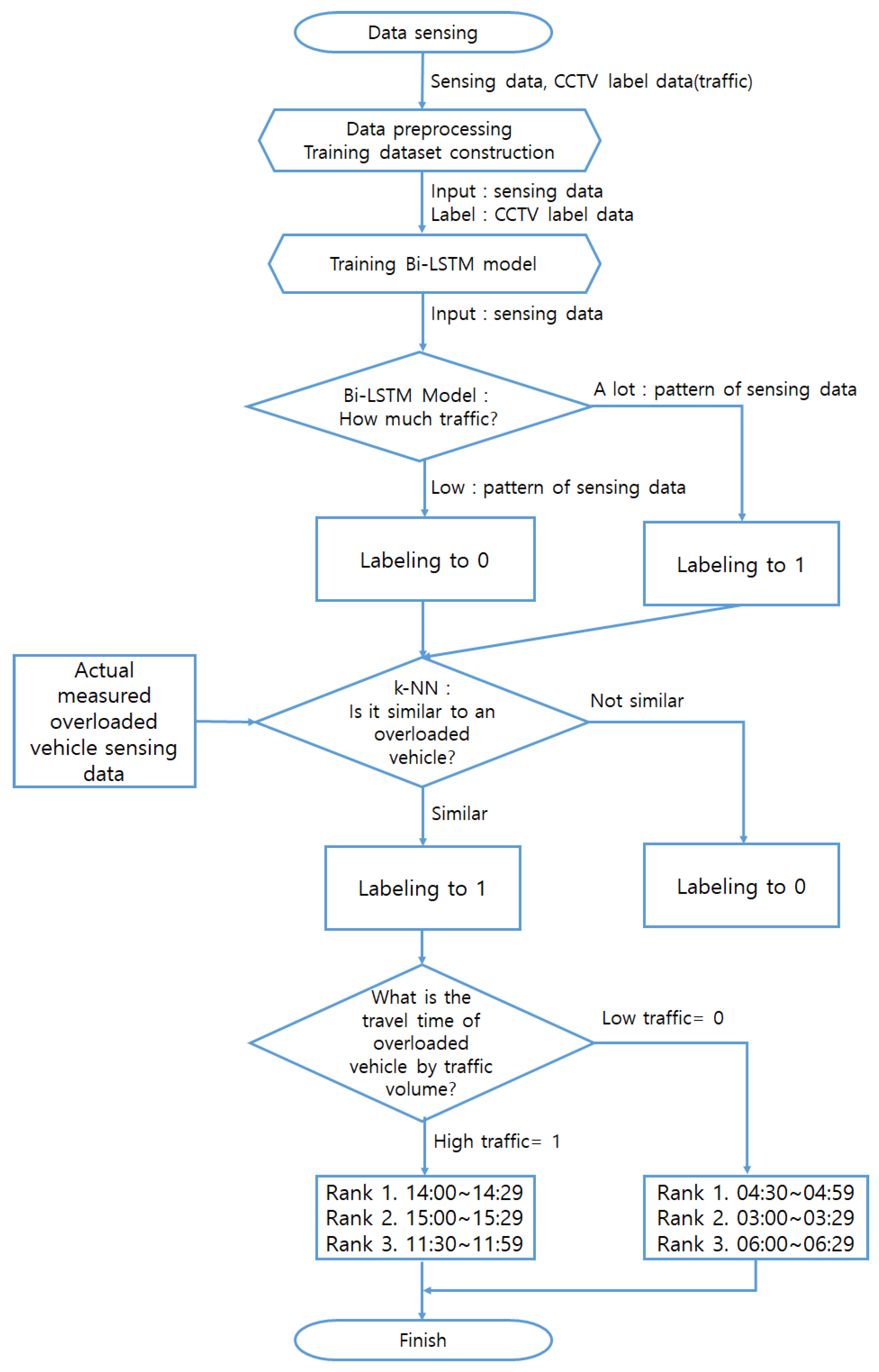
To solve the problem of identifying the top-k time zones with many overloaded vehicles in a bridge, we propose the novel two-step approach.

In the first step, we propose a new urban bridge traffic classification model using a bidirectional long short-term memory (Bi–LSTM) that is defined in detail in Section 4.4. When a time series vector v that includes class (i.e., c = high or low traffic), time (e.g., t = 2018.09.19 00:00:01), and 9-axis acceleration/gyroscope/magnetometer sensing values (e.g., $x_1=21$, $y_1=349.63$, $z_1$ = 21,382.6, $x_2=-177.94$, $y_2=65.74$, $z_2=78.74$, and $z_3=2488.32$) is given as an input, the proposed deep learning-based model is learned in the training step and automatically classifies a new $v_t$ 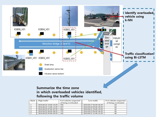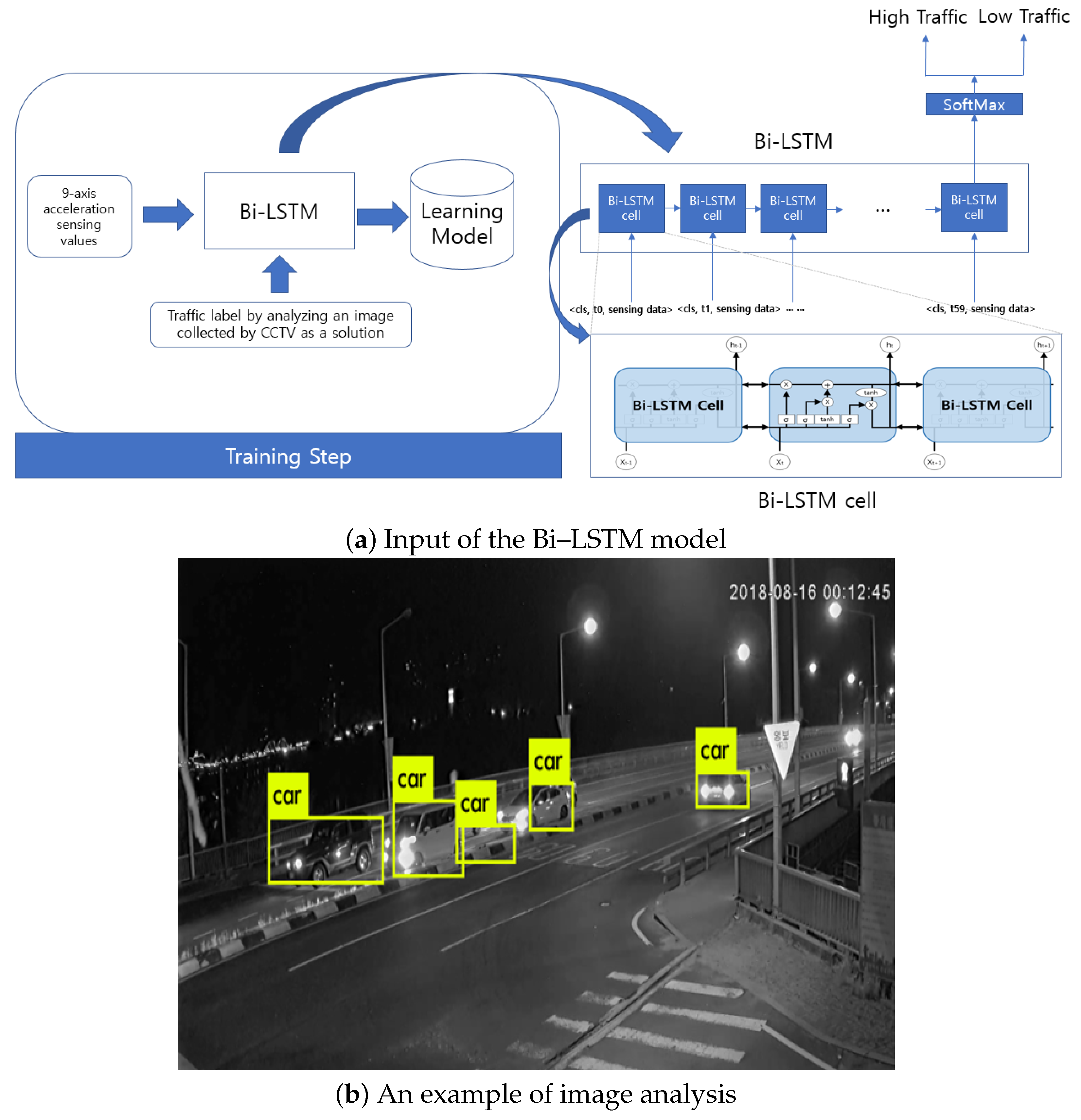to either high or low traffic in the test step. To learn the Bi–LSTM model, we prepare the label set using the results of analyzing the images collected from CCTV installed on the bridge.

In the second step, the proposed model automatically finds the top-k time zones with many overloaded vehicles in the high traffic cluster. For this, we propose a new automatic method of identifying the top-k time zones using k-Nearest Neighbor (NN). With the cooperation of the Urban Transit Bureau, we rented a freight vehicle with more than 40 tons, and measured the 9-axis acceleration/gyroscope/magnetometer-sensing values when the cargo truck passed through the bridge. These measured values are called the solution set S. Through statistical verification, we observed that the difference in the sensed values between the overloaded and nonoverloaded vehicles is statistically significant. Finally, all vectors in the high traffic cluster are assigned to 48 time zone units, each of which corresponds to 30 min. The k-NN method is used to calculate the similarity between the sensing values of S and the vectors belonging to each time zone, and then identifies k best time zones similar to S.

Figure 1 shows the overall process of the proposed model. Before describing the proposed methods in detail, we will first discuss the basic hypothesis of the proposed model and the preprocessing method for cleaning raw data in the next subsections.

4.1. Our Hypothesis

In this section, we describe in detail our main idea that overloaded vehicles can be detected using various inexpensive general-purpose IoT sensors because of the difference in the sensed values between the overloaded and nonoverloaded vehicles.

The 9-axis sensor we used consists of a 3-axis acceleration sensor ($x_1$, $y_1$, and $z_1$), a 3-axis gyroscope sensor ($x_2$, $y_2$, and $z_2$), and a 3-axis magnetometer sensor ($x_3$, $y_3$, and $z_3$). KSB01_V01, KSB02_V01, KSB03_V01, KSB04_V01, KSB05_V01, and KSB06_V01 are six 9-axis sensors installed in Wonchon Bridge.

In the 3-axis acceleration sensor, the acceleration is the rate of change of velocity of an object with respect to time. For example, a car that moves 100 km at $t_1$ time and 110 km at $t_2$ time has an acceleration of 10 km. In this case, the driver stepped on the accelerator to increase engine combustion and generate 10 km of force. The $x_1$-axis is horizontal to the lane, the $y_1$-axis is orthogonal to the $x_1$-axis on the plane, and the $z_1$-axis is orthogonal to the plane. The 3-axis acceleration sensor emits ultrasonic waves in the $x_1$-, $y_1$-, and $z_1$-axis directions and calculates the velocity by calculating the return value of the object. Then, it calculates the acceleration by differentiating the velocity with time. In general, since most vehicles entering the bridge do not accelerate, the value of the $x_1$-axis is constant regardless of the overloaded and the nonoverloaded vehicles. Also, as the $y_1$-axis is orthogonal to the $x_1$-axis, the $y_1$-axis is also meaningless. Compared to a nonoverloaded vehicle, when an overloaded vehicle passes by the bridge, the bridge is slightly shaken down by its weight. Acceleration is caused by an artificial force or by the mass of an object. As the overloaded vehicle has a larger mass than the nonoverloaded vehicle, a large force is generated when the overload vehicle passes, affecting the $z_1$-axis of acceleration.

In the 3-axis gyroscope sensor, when there are 3-axis coordinate systems ($x_2$, $y_2$, and $z_2$) and tilted 3-axis coordinate systems ($x_2^{\prime }$, $y_2^{\prime }$, and $z_2^{\prime }$), each pair such as $x_2$ and $x_2^{\prime }$, $y_2$ and $y_2^{\prime }$, and $z_2$ and $z_2^{\prime }$ is connected by a spring. Since most overloaded vehicles are larger and heavier than small cars, shaking is greatly detected in all directions such as $x_2$, $y_2$, and $z_2$ axes. For this reason, the values of the $x_2$, $y_2$, and $z_2$ axes generated when the overloaded vehicle passes the bridge are different from those generated when the nonoverloaded vehicle passes.

In the 3-axis magnetometer sensor, the $x_3$-axis is horizontal to the lane, the $y_3$-axis is orthogonal to the $x_3$-axis on the plane, and the $z_3$-axis is orthogonal to the plane. The $x_3$-axis means the north and south directions of the magnet. The $y_3$-axis means the east and west directions of the magnet. The $z_3$-axis means up and down. Regardless of the type of vehicle, it does not affect the magnetometer. Compared to a nonoverloaded vehicle, when an overloaded vehicle passes by the bridge, the bridge is slightly shaken down by its weight. The closer we are to the center of the earth, the stronger the magnet. Therefore, the value of the $z_3$-axis increases when the bridge is slightly shaken down as the overloaded vehicle passes.

Our approach is reasonable because the experimental result shows the sensing values of the $x_1$, $y_1$, $z_1$, $x_2$, $y_2$, $z_2$, $x_3$, $y_3$, and $z_3$ axes as the overloaded and nonoverloaded vehicles pass over the bridge. As described above, the values of $z_1$, $x_2$, $y_2$, $z_2$, and $z_3$ generated when the overloaded vehicle passes by are significantly different from those of the nonoverloaded vehicle. As shown in

Table 2. Magnitude of the average difference in sensed values. 

Vehicle	${\mathit{z}}_1$	${\mathit{x}}_2$	${\mathit{y}}_2$	${\mathit{z}}_2$	${\mathit{z}}_3$	Average
Overloaded	3620	3620	3650	3630	4000
Nonoverloaded	2500	2500	2500	2800	2600
Difference rate	0.448	0.448	0.46	0.296	0.538	0.438

, the magnitude of the average difference in the sensed values between the overloaded and nonoverloaded vehicles is about 44%. These results strongly support our hypothesis. Specific experimental results will be described in the Experimental Results section.

4.2. Preprocessing Raw Sensing Data

In this section, we discuss the preprocessing method for generating the input data of the bridge traffic classification model. As described in Section 4.1, seven meaningful sensing values collected from two sensors close to CCTV (KSB02 and KSB05) are aggregated into one-minute units to create an input vector of the proposed model.

Each sensor installed in a bridge collects the sensing values shown in

Table 3. An example of the sensing values used in the experiment. 

Type	Sensor	Sensor Value
Sensor name	SEN_INFO	KSB05_V01
Date	DATE	2018–09–18T15:21:30
Temperature	TEMP	30.6
Humidity	HUMI	34.4
3-axis acceleration (LIS344)	f	2
	x	2034
	y	2002
	z	2896
9-axis acceleration /gyroscope/ magnetometer (LSM9DS1)	$f_1$	2
	$x_1$	70
	$y_1$	326
	$z_1$	20,823
	$f_2$	433
	$x_2$	−154
	$y_2$	21
	$z_2$	−30
	$f_3$	−20
	$x_3$	−65,535
	$y_3$	−65,535
	$z_3$	2283
Vibration	GALS	0
GPS	n	3622.736
	e	12,724.54
	m	120
Speedometer (GRM-K600WP)	GRM	45

, every 0.1 s. The reason for preprocessing such raw data is to remove the meaningless sensing values for a bridge traffic classification model. First, the sensors’ values that are not directly related to traffic classification are deleted. Accordingly, the values of the temperature and humidity sensors are removed. GPS information is also not needed for the bridge traffic classification model. As the F–value of the 3-axis acceleration sensor is always 2, it is not suitable for use in the proposed model. For instance, LIS344_f = ‘2’ in 19 September 2018 00:21, LIS344_f = ‘2’ in 19 September 2018 00:22, LIS344_f = ‘2’ in 19 September 2018 00:23, and so on. Meanwhile, the sensor information such as ‘KSB05’ is removed in the preprocessing step. In addition, the sensing value that is repeated in a certain order is removed. For example, the $F_2$–value of the 9-axis acceleration/gyroscope/magnetometer sensor is a simple repetition of 0∼999 without a meaningful pattern—e.g., LSM9DS1_$f_2$ = ‘998’ in 19 September 2018 00:21, LSM9DS1_$f_2$ = ‘999’ in 19 September 2018 00:22, LSM9DS1_$f_2$ = ‘0’ in 19 September 2018 00:23, LSM9DS1_$f_2$ = ‘1’ in 19 September 2018 00:24, and so on.

The 9-axis sensors generate sensing values of nine axes—$x_1$, $y_1$, $z_1$, $x_2$, $y_2$, $z_2$, $x_3$, $y_3$, and $z_3$—every 0.1 s. However, $x_3$ and $y_3$ are excluded because they continue to generate meaningless values of −65,535. In addition, as each sensing value is collected every 0.1 s and most sensing values have the same value, ten sensing values are aggregated in 1 s. For example, the average of ten sensing values of $x_1$ corresponding to one second is computed and stored to the database.

To learn the bridge traffic classification model, we generate the label set by using images in CCTV installed in the bridge. With YOLO—the latest image processing technology [13]—when an image is given as input, the numbers of cars, buses, and trucks are automatically counted as the output. These results are collected every minute. Therefore, in order to match the measurement time unit with the image data collected every minute, the 9-axis sensing value collected every 0.1 s should be aggregated in 1 min. In other words, the average value of the sensing values collected between YYYY:MM:DD HH:MM:00 second and YYYY:MM:DD HH:MM:59 second is calculated as a sensing value in unit of one minute.

The CCTV data is used to measure the number of vehicles passing through, taking into account both lanes of the bridge. Therefore, the average of the sensing values of both sides is calculated as a single sensed value. For instance, assume the following sensing values.

• SEN_INFO = ‘KSB02’, DATE = ‘2018:09:19 00:01:01’, LSM9DS1_$y_2$ = ‘74.75’, ...
• SEN_INFO = ‘KSB05’, DATE = ‘2018:09:19 00:01:01’, LSM9DS1_$y_2$ = ‘68.65’, ...
• SEN_INFO = ‘KSB02’, DATE = ‘2018:09:19 00:01:02’, LSM9DS1_$y_2$ = ‘60.14286’, ...
• SEN_INFO = ‘KSB05’, DATE = ‘2018:09:19 00:01:02’, LSM9DS1_$y_2$ = ‘61.75’, ...

KSB02 is the sensor that measures the upstream vehicles of the bridge, and KSB05 is the sensor that measures the downstream vehicles of the bridge. The above sensing values are merged as follows.

• SEN_INFO = ‘KSB02+KSB05’, DATE = ‘2018:09:19 00:01:01’, LSM9DS1_$y_2$ = ‘71.7’, ...
• SEN_INFO = ‘KSB02+KSB05’, DATE = ‘2018:09:19 00:01:02’, LSM9DS1_$y_2$ = ‘60.94643’, ...

Then, sensing values from YYYY:MM:DD HH:MM:01 second to YYYY:MM:DD HH:MM:59 second are aggregated into a one-minute sensing value and expressed in one row as follows.

• SEN_INFO = ‘KSB02+KSB05’, DATE = ‘2018:09:19 00:01’, LSM9DS1_$y_2$ = ‘72.7’, ...
• SEN_INFO = ‘KSB02+KSB05’, DATE = ‘2018:09:19 00:02’, LSM9DS1_$y_2$ = ‘70.3’, ...
• SEN_INFO = ‘KSB02+KSB05’, DATE = ‘2018:09:19 00:03’, LSM9DS1_$y_2$ = ‘72.7778’, ...

4.3. Preparation of Train Set for Bridge Traffic Classification Model Using Bi–LSTM

In this section, we describe how to generate training data for the proposed model. Using YOLO [13], the numbers of cars, trucks, and buses are automatically extracted from an image for a specific time. Based on this extracted information, the high or low traffic of each time is labeled and used as the class value of the input vector. Each input vector consists of class, time, and seven sensing values such as $x_1$, $y_1$, $z_1$, $x_2$, $y_2$, $z_2$, and $z_3$. These input vectors are gathered to form the train set.

We automatically measure the numbers of vehicles, buses, and trucks from the image generated every minute from CCTV installed on the bridge, using the latest image processing technique [13]. We can also calculate the total weight of a bus when the passenger is full on the bus as follows:

$$\mathrm{Total} \mathrm{weight} \mathrm{of} \mathrm{a} \mathrm{bus}=\mathrm{Weight} \mathrm{of} \mathrm{the} \mathrm{bus} \mathrm{itself}+\mathrm{Max} \mathrm{number} \mathrm{of} \mathrm{passengers}\times \mathrm{Average} \mathrm{weight} \mathrm{of} \mathrm{an} \mathrm{adult}$$

(1)

For instance, the total weight of a bus is computed by 15,000 kg + (70 × 75 kg ) = 20.250 kg. That is, the total weight of the bus when the passenger is full is ~20.2 tons. Although the weight of a bus is only 0.5 times lower than the weight of an overloaded vehicle, the vibrations occurring in large buses are expected to be similar to those of the overloaded vehicle due to passenger motion. That is why we extract data for trucks and buses with a measured ratio of 7:3 or more (Through repeated experiments with various ratios, we observed that the deep learning model had the highest accuracy at a 7 to 3 ratio). The reason why we added sensing values for buses that are not related to overloaded vehicles in the training data is to increase the accuracy of the deep learning model by adding noise values. This is like a dropout effect in deep learning models. The bus is half the weight of an overloaded vehicle, but if it is full, passengers will be more likely to shake the bridge as much as an overloaded vehicle. If the sum of the numbers of cars, trucks, and buses in an image is less than 10, the traffic condition shown in the image is considered to be low (0) and the traffic condition is high (1), otherwise. The followings are the examples of the label set in order to learn the bridge traffic classification model.

• DATE = ‘2018:09:19 00:01’, # of cars = 12, # of buses = 2, # of trucks = 7, Sum = 21, Class = 1
• DATE = ‘2018:09:19 00:02’, # of cars = 15, # of buses = 1, # of trucks = 1, Sum = 17, Class = None
• DATE = ‘2018:09:19 00:03’, # of cars = 6, # of buses = 0, # of trucks = 4, Sum = 10, Class = 0

Please take a look at the second data in 2018.09.19 00:02. The value of the class is none because the ratio of cars and buses to trucks does not satisfy 3:7. Therefore, the sensing data corresponding to Class = None are removed. The following data is the final train set for Bi–LSTM.

• DATE = ‘2018:09:19 00:01’, LSM9DS1_$y_2$ = ‘71.7’, ..., Class = 1
• DATE = ‘2018:09:19 00:03’, LSM9DS1_$y_2$ = ‘72.7778’, ..., Class = 0

4.4. Bridge Traffic Classification Model Using Bi–LSTM

In this section, we propose a Bi–LSTM-based bridge traffic classification model. Most previous studies for traffic detection are based on correlation analysis, vehicle–to–vehicle communication, and simple statistical techniques. Recently, a simple application of machine learning or deep learning techniques has been proposed, but the characteristics of time-series data such as sensing values generated in real time are not considered. To surmount the disadvantage of the previous methods, we propose a deep learning model that classifies traffic condition well by considering time series sensing values collected from the bridge.

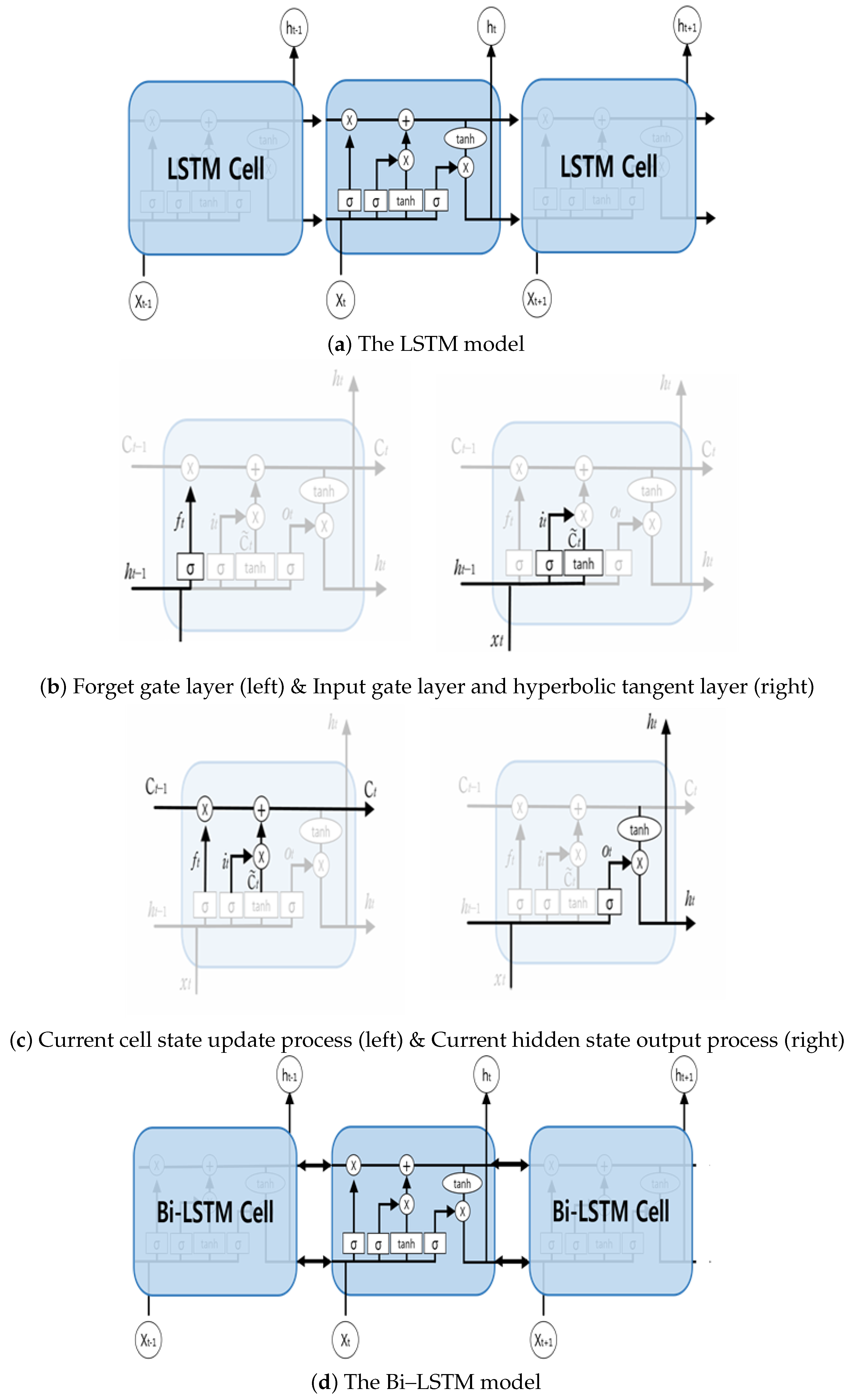
As the inputs of the bridge traffic classification model are time series data, we consider the Recurrent Neural Networks (RNN) model among various deep learning models. The RNN model is learned by considering the order of input data such as sequence data, natural language processing, and machine translation. For example, when there is a sentence such as, “I eat bread before going to school every day and I drink milk together,” the word “milk” that appears after the drink will have a relatively higher probability than other word such as “gasoline”. Thus, the words “milk” and “drink” do not appear independently of each other, but the probability of generating ‘milk’ is affected by the word “drink”. As the hidden layers of an artificial neural network are piled up deeply, there is the gradient vanishing problem which results in much less accuracy of backpropagation. To address the problem, new activation functions such as rectified linear unit (ReLU) and hyperbolic tangent (tanh) have been used instead of the sigmoid function. However, the disadvantage of these functions is that short-term memory is possible, but long-term memory is not. In the above sentence, if the information of bread is far away to infer milk, it is difficult to carry this information far enough with the RNN. In our problem, 60 sensing values, each of which is created per second, are given as inputs to the RNN model. If the 0th sensing value is important for inferring the 59th sensing value, since the two values are far away, the 0th sensing value is likely to disappear in the middle, and the accuracy of the RNN model will decrease. The objective of the Long Short-Term Memory (LSTM) model [14] is to create a separate cell for information that requires long-term memory in Figure 2a. Also, if the 15th sensing value is not important to infer the 59th sensing value, it should be forgotten in the middle. Thus, since LSTM separates $c_t$ information to be stored in a cell and $h_t$ information to be output, the forget and input gates are added to the cell.

The core of the LSTM is a cell state, and the cell state is composed of a forget gate layer, an input gate layer, and a hyperbolic tangent layer. Through this, LSTM is a model for selecting only useful information by forgetting unimportant information and memorizing important information among the previous information. Figure 2b shows the process for the forget gate layer, the input gate layer, and the hyperbolic tangent layer. The forget gate layer is the process of selecting which information to discard in the cell state. It takes the Sigmoid function from the previous hidden state and the current input. If the output value is 0, it means to discard this value completely. If it is 1, it means to keep this value completely. $f_t$ is expressed by the following equation.

$$f_t=\sigma (W_f*[h_{t-1},x_t]+b_f)$$

(2)

The input gate layer, $i_t$, receives $h_{t-1}$ and $x_t$ as inputs and determines which value to update. Next, the hyperbolic tangent layer $\widetilde{C_t}$ produces a value that can be added to the cell state. $i_t$ is multiplied by $\widetilde{C_t}$ to affect the next state. The formula is as follows.

$$i_t=\sigma (W_i*[h_{t-1},x_t]+b_i)$$

(3)

$$\widetilde{C_t}=tanh(W_C*[h_{t-1},x_t]+b_C)$$

(4)

Figure 2c shows the process of updating the previous cell state to the current cell state and the process of outputting the current hidden state. The current cell state $C_t$ is the sum of the product of the forget gate cell $f_t$ and the previous cell state $C_{t-1}$ and the product of the input gate layer $i_t$ and the hyperbolic tangent layer $\widetilde{C_t}$. The equation for $\widetilde{C_t}$ is as follows.

$$\widetilde{C_t}=f_t*C_{t-1}+i_t*\widetilde{C_t}$$

(5)

Finally, we decide on the current hidden state ($h_t$). The current hidden state is determined through the following process; $h_{t-1}$ and $x_t$ are input, and $o_t$ is obtained through the Sigmoid function. Next, we extract the value between −1 and 1 through the hyperbolic tangent function and $o_t$ is multiplied by $tanh\left(C_t\right)$. The formula for $h_t$ is as follows.

$$o_t=\sigma (W_o*[h_{t-1},x_t]+b_o)$$

(6)

$$h_t=o_t*tanh\left(C_t\right)$$

(7)

The Bi–LSTM model has the same principle as the LSTM model, but differs from the LSTM model in that the input information is processed in both directions rather than forward direction. Figure 2d shows that Bi–LSTM has an advantage in that it can find patterns that cannot be found by only one direction, because Bi–LSTM considers input information in both directions of forward and backword. In fact, comparing the accuracy of the Bi–LSTM model with that of the LSTM model, the Bi–LSTM model showed 0.5 times higher accuracy than the LSTM model.

4.5. Automatic Method for Identifying Top-k Time Zones with Many Overloaded Vehicles

In this section, we present a new k-Nearest Neighbor (NN)-based [15] method that automatically finds the top-k time zones with many overloaded vehicles in the high traffic cluster. With the cooperation of the Urban Transit Bureau, we rented freight vehicles with more than 40 tons, and measured the 9-axis acceleration/gyroscope/magnetometer-sensing values when the cargo truck passed through the bridge. These measured values are called the solution set S. Through statistical verification, we found that the difference in the sensing values between the overloaded and nonoverloaded vehicles is statistically significant. The results will be discussed in detail in the Experimental Results section.

For example, to determine if the sensed values generated on a particular time are relevant to the overloaded vehicle, we first create the following comparison set $\{e_1,e_2,e_3,e_4\}$.

• $e_1$: DATE = ‘2018.09.19 14:25:03’, LSM9DS1_$y_1$ = ‘448’, LSM9DS1_$z_3$ = ‘2,296’ (from S)
• $e_2$: DATE = ‘2018.09.19 15:11:45’, LSM9DS1_$y_1$ = ‘439’, LSM9DS1_$z_3$ = ‘2,278’ (from S)
• $e_3$: DATE = ‘2018.09.19 16:12:12’, LSM9DS1_$y_1$ = ‘287’, LSM9DS1_$z_3$ = ‘2,246’ (from $S^c$)
• $e_4$: DATE = ‘2018.09.19 16:28:11’, LSM9DS1_$y_1$ = ‘320’, LSM9DS1_$z_3$ = ‘2,270’ (from $S^c$)

The ratio of the elements from S to ones from $S^c$ is 50:50 in the comparison set. Please note $S^c=\{x\in Ux\ni S\}$, where U is a universal set. Given $e_q$: DATE = ‘2018.09.19 17:01:11’, LSM9DS1_$y_1$ = ‘446’, LSM9DS1_$z_3$ = ‘2,286’, the distance between $e_{i=1,2,3,or4}$ and $e_q$ is calculated by Euclidean distance.

• $dist(e_1,e_q)=\sqrt{{(448-446)}^2+{(2,296-2,286)}^2}=10.2$
• $dist(e_2,e_q)=\sqrt{{(439-446)}^2+{(2,278-2,286)}^2}=10.6$
• $dist(e_3,e_q)=\sqrt{{(287-446)}^2+{(2,246-2,286)}^2}=163.9$
• $dist(e_4,e_q)=\sqrt{{(320-446)}^2+{(2,270-2,286)}^2}=127.0$

If the distance between $e_i$ and $e_q$ is close to 0, it means that $e_i$ and $e_q$ are identical. When $k=3$, top-3 distances with the lowest values such as $dist(e_1,e_q)$, $dist(e_2,e_q)$, and $dist(e_4,e_q)$ are selected. $e_1$ and $e_2$ are the sensed values which are relevant with the overloaded vehicles but $e_4$ is not. By a majority vote, $e_q$ is determined as the sense value that is relevant with the overloaded vehicle.

Finally, all vectors in the high traffic cluster are assigned to 48 time zone units, each of which corresponds to 30 min. The k-NN method is used to calculate the distance between the values of S and the sensing values belonging to each time zone, and then identify k best time zones similar to S.

5. Experimental Set-Up

5.1. Test Bed for our Experiment

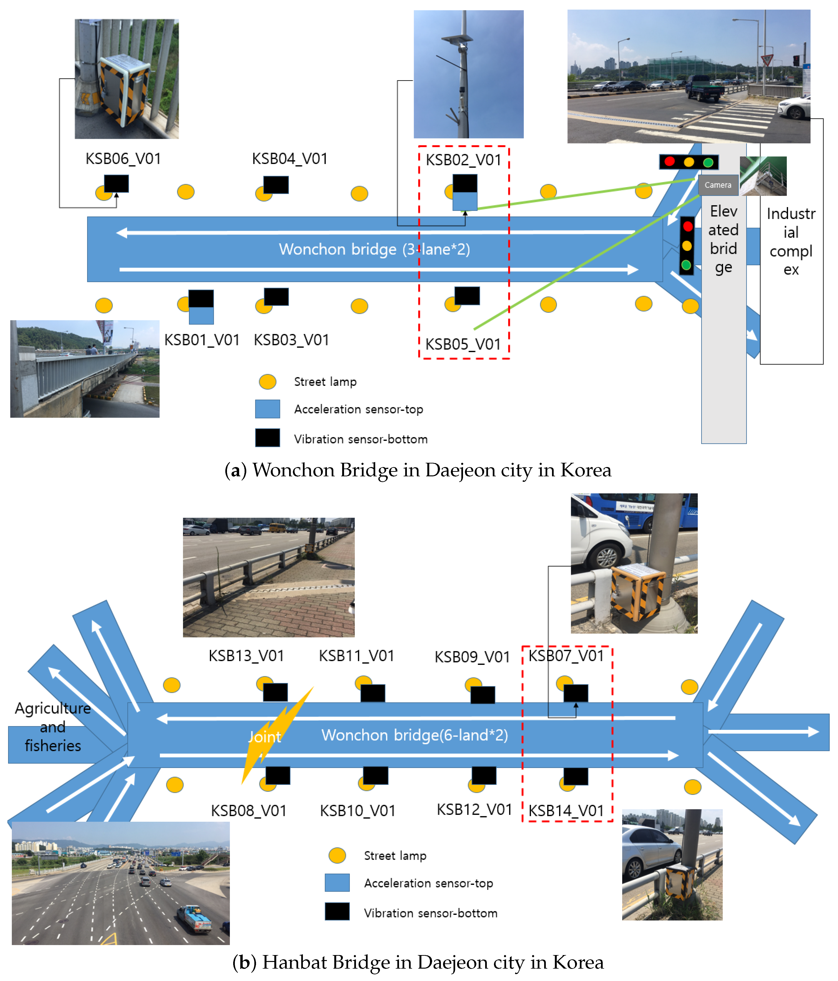
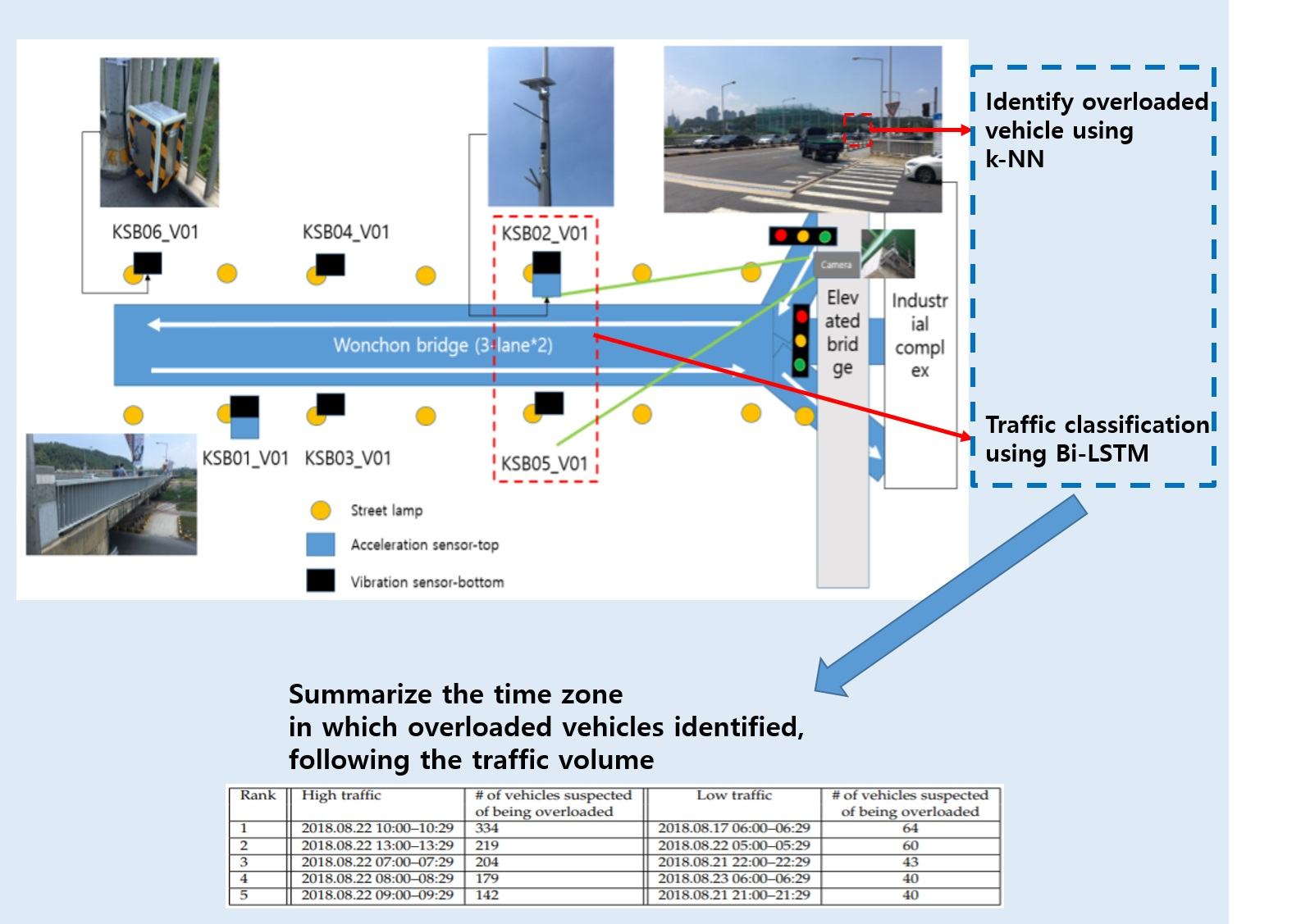
In this section, we describe the details of sensors and CCTV installation on two bridges for the experiment. IoT sensors were installed in two major bridges in Daejeon city in central part of Korea. As shown in Figure 3a, there is a total of six boxes including various sensors and one CCTV in the Wonchon bridge. In the figure, KSB01_V01–KSB06_V01 are such boxes. Each box includes a temperature and humidity sensor (SHT35), a nine-axis acceleration/gyroscope/magnetometer sensor (LSM9DS1), a vibration sensor (D7E–2), latitude/longitude/altitude information (GPS), and a speedometer (GRM–K600WP). However, three-axis acceleration sensors were additionally installed in KSB01_V01 and KSB02_V01 boxes only. In addition, CCTV was installed on the elevated bridge to record vehicles passing through the bridge.

We used only the sensing data collected in KSB02_V01 and KSB05_V01 for traffic prediction. The reason for choosing such sensors is that the label data extracted from the images of CCTV is more related to the sensed values collected from sensors near CCTV than other sensors. For example, if the distance between CCTV and a sensor is far apart, the accuracy of the proposed model will deteriorate because of the difference between the time when the image is captured and the time of the sensing value collected by the sensor.

Figure 3b shows the sensors in the Hanbat bridge, another main bridge in Daejeon city. A total of eight boxes including the same sensors installed in the Wonchon bridge except a three-axis acceleration sensor was installed in the bridge but any CCTV is not there. KSB07_V01–KSB14_V01 are such boxes in the figure. Hanbat Bridge did not have CCTV installed, so we could not make label data necessary for learning Bi–LSTM. Therefore, we used the label data made by CCTV of Wonchon Bridge to learn the traffic prediction model of Hanbat Bridge.

Hanbat Bridge has a singularity point called a seam on the bridge. Since sensors around the seam can act sensitively in the process of gathering sensing data, the sensed data are likely to contain noise, which will prevent Bi–LSTM from being learned properly. To deal with this problem, we used only the sensing data collected in KSB07_V01 and KSB14_V01. Such sensors are expected to be least affected by the seam because they were installed at the farthest point away from the seam.

5.2. Preprocessing Sensing Data

In this section, we describe the details of the preprocessing method for the experiment. First, we transform the sensing values collected from the sensors to the input data of the Bi–LSTM model. The objective of the first preprocessing step is to remove the values of $f_1$, $f_2$, $f_3$, $x_3$, and $y_3$ of LSM9DS1, in addition to GRM and GALS. The reason is that the value of the vibration sensor is measured as zero all the time because it is too insensitive. In the second preprocessing step, we removed the DATE and SEN_INFO fields. In the third step, we removed the $F_2$ values of LSM9DS1 because the sensing value is repeated from 0 to 999 without special meaning. In the fourth step, we deleted all GPS information and all values of TEMP, HUMI, and LIS344 in the last step. The reason for removing the values of LIS344 is: As we mentioned before, we merely consider two sensor boxes—KSB02_V01 and KSB05_V01 in Wonchon Bridge. Please note that there is a three-axis acceleration sensor in KSB02_V01, but no such a sensor in KSB05_V01. As the label data is the number of vehicles passing through the bridge considering both lanes, the sensing data of both sensors are also converted into a single sensing data through the average value. Since the same sensors must be existed in both lanes, but a 3-axis acceleration sensor is not in KSB05_V01, the average of the sensing values in both lanes cannot be calculated. In addition, the sensing values collected from the temperature and humidity sensor are removed because they are not directly related to the problem. After the preprocessing step, a total of seven sensing values are prepared for learning Bi–LSTM. These sensing values are $x_1$, $y_1$, $z_1$, $x_2$, $y_2$, $z_2$, and $z_3$ values of the nine-axis acceleration/gyroscope/magnetometer sensor (LSM9DS1). We collected the sensed values of the nine-axis acceleration/gyroscope/magnetometer sensors in Wonchon Bridge from 5 August 2018 to 23 August 2018 and in Hanbat Bridge from August 15, 2018 to 23 August 2018.

5.3. Generating Train Set for Bridge Traffic Classification Model

In this section, we describe the implementation details of the bridge traffic classification model for the experiment. Figure 4 shows how to learn the bridge traffic classification model using Bi–LSTM. We prepared a train set in which there are 3320 input vectors created by the sensors in Wonchon Bridge and a validation set in which there are 830 input vectors. Then, we created four test sets of data, each with 5300 input vectors. In Figure 4a, each input vector of Bi–LSTM is composed of class (cls), time ($t_{i=\{0,1,\dots ,59\}}$), and seven sensing values ($x_1$, $y_1$, $z_1$, $x_2$, $y_2$, $z_2$, and $z_3$ values of the nine-axis acceleration/gyroscope/magnetometer sensor). The class is either 1 or 0, meaning that 1 is high traffic and 0 is low traffic. The class value is determined by analyzing the image that is generated in the same time as the sensing values. Using one of existing image processing techniques, the numbers of cars, buses, and trucks per image are counted automatically. Figure 4b shows that five cars are automatically identified in an image on 16 August 2018 at 00:12:45. Finally, if the sum of the numbers of cars, trucks, and buses in the image is less than 10, the traffic condition shown in the image is considered to be low (0) and the traffic condition is high (1), otherwise.

5.4. Actual Measurement of Nine-Axis Sensing Values about an Overloaded Vehicle

In this section, we describe the details of actual measurement of nine-axis sensing values about an overloaded vehicle for the experiment. To identify vehicles that are suspected to be overloaded, it is necessary to measure the 9-axis sensing values when the actual overloaded vehicle passes through the bridge. For this, we collected the 9-axis sensing values that were generated when the overloaded vehicle passed through the bridge on 19 September 2018 from 14:00 to 15:30. The actual measurement data has time series data characteristics. The number of the instance vectors is 50 and the number of the vector dimensions is 9. Each value of the vectors is real number.

Table 4. An example of actual sensing values related to an overloaded vehicle. (The values in bold are the sensing values when the overloaded vehicle passed through the bridge.) 

Date	${\mathit{x}}_1$	${\mathit{y}}_1$	${\mathit{z}}_1$	${\mathit{x}}_2$	${\mathit{y}}_2$	${\mathit{z}}_2$	${\mathit{z}}_3$
19 September 2018 15:11:31	130.375	175.25	2740.375	2716.625	2713.5	2716.875	2992.625
19 September 2018 15:11:32	149.2222	205.5556	2506.556	2490.222	2501.444	2514	2759.111
19 September 2018 15:11:33	150.5556	181.4444	2493.556	2473.667	2473.889	2483	2728.889
19 September 2018 15:11:34	97.33333	184.6667	3642.5	3614.833	3616	3627.667	3995.667
19 September 2018 15:11:35	33.22222	71.33333	2353.222	2336.444	2340	2346.889	2591.556
19 September 2018 15:11:36	100.5556	159.6667	2450.222	2431.222	2429.778	2436.111	2682.111
19 September 2018 15:11:37	88.11111	129.6667	2451.333	2429.222	2430.111	2436.222	2682

shows an example of measuring real values of a nine-axis sensor related to the overloaded vehicle. The table shows the difference between the 9-axis sensing values when the actual overload vehicle passes and when it does not. Although the $x_1$ and $y_1$ axis values are not significantly different, we observed that there is a difference among the sensing values of $z_1$, $x_2$, $y_2$, $z_2$, and $z_3$ axes.

5.5. Implementation

In this section, we describe the details of computer hardware and software for the experiment. All the experiments were performed on a workstation server with Intel(R) Core(TM) i7-4790 CPU @ 3.60 GHz processor, 32 GB of RAM, and 1TB of HDD, running on Ubuntu 15.10 as OS. We implemented the preprocessing step, bridge traffic classification model using Bi–LSTM, and k-NN based top-k time zones identification method in Python (version 3.4) and TensorFlow (version 0.9.1). We also used IBM–SPSS Statistics 21 for the t-tests.

6. Experimental Results

6.1. Correlation between the Sensing Value and the Overloaded Vehicle

In this section, we used the independent sample t-test to verify that there is a large difference between the sensing values of overloaded and nonoverloaded vehicles. We also examined how much two evaluators agree on the difference between sensing values of overloaded and nonoverloaded vehicles. Two experimental results clearly show that there is a difference in the sensing information of overloaded and nonoverloaded vehicles.

Firstly, we used a statistical test to investigate whether there is a high correlation between the overloaded vehicle and the 9-axis acceleration/gyroscope/magnetometer sensing value. In other words, it is necessary to statistically verify whether there is always a large difference in the sensed values of the overloaded and nonoverloaded vehicles. To do this, we firstly determine whether there is a significant difference between the sensed values of the overloaded and nonoverloaded vehicles through independent sample t-test. The null hypothesis $H_0$, the alternative hypothesis $H_1$, and the significance level $\alpha =0.05$ are as follows.

• $H_0$: ${\mu }_1-{\mu }_2=0$, $H_1$: ${\mu }_1-{\mu }_2\ne 0$

$H_0$ indicates that there is no difference between the average sensed value (${\mu }_1$) of overloaded vehicles and that (${\mu }_2$) of nonoverloaded vehicles, and $H_1$ indicates that there is difference between the average sensed value (${\mu }_1$) of overloaded vehicles and that (${\mu }_2$) of nonoverloaded vehicles.

Table 5. Independent sample t-test to verify the correlation between the sensing value and the overloaded vehicle.

		Test of Equal Variances in Levene		t-Test for Equality of Means
		F	p-Value	t	Degree of Freedom	Sig. Prob. (both)	Mean	Standard Error of Difference	95% Confidence Intervals of Difference
							Differ.		Lower limit	Upper limit
$z_3$	Equal variance assumed	0.044	0.842	2.905	5	0.034	25.6891	8.84250	2.95876	48.41948
	Equal variance not assumed			2.967	4.758	0.033	25.6891	8.65946	3.08491	48.29333

shows the results for the independent sample t-test. As the probability of significance is less than 0.05, the null hypothesis is rejected and the alternative hypothesis is adopted. This is, unlike nonoverloaded vehicles, the sensed values of overloaded vehicles have a statistically significant difference.

Secondly, two evaluators manually take a look at the sensing information and answer whether the vehicle corresponding to the sensing information is overloaded or not, and the agreement degree of their answers is measured by Kappa coefficient. The higher the Kappa coefficient, the higher the agreement between the two evaluators. For the experiment, two volunteers who had nothing to do with this work participated in the test and sensing information was randomly extracted from the sensing information generated when the actual overloaded vehicle passed through the bridge. Likewise, sensing information was randomly extracted from the sensing information generated when the nonoverloaded vehicle passed through the bridge. In order to obtain the Kappa coefficient, we randomly selected sensing information related to three overloaded vehicles and sensing information related to seven nonoverloaded vehicles. The equation for the Kappa correlation coefficient is

$$\mathrm{Kappa}=\frac{Pr\left(a\right)-Pr\left(e\right)}{1-Pr\left(e\right)}$$

(8)

$Pr\left(e\right)$ is the probability of dividing the number of answers matched by the two evaluators’ answers into the total number of cases. For example, referring to

Table 6. Excessive vehicle judgement of evaluator 1 and evaluator 2.

		Evaluator1
		Overloaded Vehicle	Nonoverloaded Vehicle
Evaluator2	Overloaded vehicle	5	1
	Nonoverloaded vehicle	0	4

, $Pr\left(e\right)=\frac{5+4}{10}=0.9$. $Pr\left(e\right)$ is composed of both the probability ($P{r}_1\left(e\right)$) that each evaluator o responded to the overloaded vehicle and the probability ($P{r}_2\left(e\right)$) that o responded to the nonoverloaded vehicle. For example, in Evaluator 1, $P{r}_1\left(e\right)=\frac{5}{10}\times P{r}_2\left(e\right)=\frac{5}{10}=0.25$. In Evaluator 2, $P{r}_1\left(e\right)=\frac{5}{10}\times P{r}_2\left(e\right)=\frac{4}{10}=0.2$. Thus, $Pr\left(e\right)=0.25+0.2=0.45$ in both Evaluator 1 and 2. In Equation (8), $\mathrm{Kappa}=\frac{Pr\left(a\right)-Pr\left(e\right)}{1-Pr\left(e\right)}=\frac{0.9-0.45}{1-0.45}=0.82$. Since the Kappa coefficient is quite high, we can conclude that the two evaluators’ answers to the sensing information related to the overloaded vehicle and the sensing information related to the nonoverloaded vehicle coincide with a high probability.

6.2. Selection of Effective Sensors in Hanbat Bridge

The independent sample t-test was performed to identify the difference between the sensing information ($s_1$) collected from the sensors far from the seam and the sensing information ($s_2$) collected near the seam. The null hypothesis $H_0$ is that there is no difference between the average ${\mu }_1$ of $s_1$ and the average ${\mu }_2$ of $s_2$, and the alternative hypothesis $H_1$ is that there is a significant difference between the average ${\mu }_1$ of $s_1$ and the average ${\mu }_2$ of $s_2$.

• $H_0$: ${\mu }_1-{\mu }_2=0$, $H_1$: ${\mu }_1-{\mu }_2\ne 0$

Table 7. Independent sample t-test to verify the effectiveness of the selected sensors in Hanbat Bridge.

		Test of Equal Variances in Levene		t-Test for Equality of Means
		F	p-Value	t	Degree of Freedom	Sig. Prob. (both)	Mean	Standard Error of Difference	95% Confidence Intervals of Difference
							Differ.		Lower Limit	Upper Limit
Sensor	Equal variance assumed	26.946	0.000	−3.082	98	0.003	−50.70	16.45292	−83.3503	−18.049
	Equal variance not assumed			−3.082	61.594	0.003	−50.70	16.45292	−83.3503	−17.807

shows the results of the independent sample t-test with the significance level $\alpha =0.05$. KSB13 is a sensor near the seam, but KSB07, KSB09, and KSB11 are sensors that are far from the seam. As a result of the independent sample t-test, the null hypothesis is adopted because the significance of the sensing data of KSB11, which is similar to the sensing data of KSB13 near the seam, exceeds 0.05. However, the null hypothesis is rejected because the significance probabilities of the sensing data of the KSB07 and KSB09, which are farthest from the sensing data of KSB13, do not exceed 0.05. The t-tests of KSB09 and KSB11 also yielded the same results. In this article, the detailed results of the KSB09 and KSB11 are omitted in terms of space limitation. As a result, the sensing data are likely to be affected by the seam. Through this statistical verification, we consider only sensing data collected from KSB07, farthest from the seam, to perform the proposed model.

6.3. Feature Selection for k-NN

Statistical verification is performed on which of the seven sensing values ($x_1$, $y_1$, $z_1$, $x_2$, $y_2$, $z_2$, and $z_3$) are proper when the k-NN method is used. The k-NN method is used to identify main time zones with many overloaded vehicles. Given two sensing information—$e_1$ and $e_2$—where $e_1$ is an input vector corresponding to the sensing data related to the overloaded vehicle, the k-NN method computes the distance between $e_1$ and $e_2$ using Euclidean Distance. For example, assuming $e_1=<x_1^{e_1},\dots ,z_3^{e_1}>$ and $e_2=<x_1^{e_2},\dots ,z_3^{e_2}>$, the distance $dist(e_1,e_2)=\sqrt{{(x_1^{e_1}-x_1^{e_2})}^2+\dots +{(z_3^{e_1}-z_3^{e_2})}^2}$. Here, we investigate that there is a high correlation among the sensing values in each feature (e.g., $x_1$).

The independent sample t-test was performed to identify the difference in the average of the sensed values of overloaded and nonoverloaded vehicles in a certain feature (e.g., $x_1$, $y_1$, ..., or $z_3$). The null hypothesis $H_0$ is that there is no difference between the averages of the sensing values in the particular feature, and the alternative hypothesis $H_1$ is that there is a significant difference between the averages of the sensing values in the particular feature

• $H_0$: ${\mu }_1-{\mu }_2=0$, $H_1$: ${\mu }_1-{\mu }_2\ne 0$

The independent sample t-test was performed at a significance level of 0.05, and the alternative hypothesis was adopted for the $y_1$ and $z_3$ features. As a result, this means that $y_1$ and $z_3$ for k-NN method are effective.

Table 8. Independent sample t-test to verify the effectiveness of the selected features for k-NN.

		Test of Equal Variances in Levene		t-Test for Equality of Means
		F	p-Value	t	Degree of Freedom	Sig. Prob. (both)	Mean	Standard Error of Difference	95% Confidence Intervals of Difference
							Differ.		Lower Limit	Upper Limit
$y_1$	Equal variance assumed	4.649	0.084	2.638	5	0.046	107.8136	40.87044	2.753	212.8745
	Equal variance not assumed			3.050	3.575	0.044	107.8136	35.35235	4.878	210.7492
$z_3$	Equal variance assumed	0.044	0.842	2.905	5	0.034	25.6891	8.84250	2.959	48.4195
	Equal variance not assumed			2.967	4.758	0.033	25.6891	8.64946	3.085	48.2933

shows the independent sample t-test results for $y_1$ and $z_3$, indicating that the t-tests of $y_1$ and $z_3$ yield similar results.

6.4. Accuracy of Bridge Traffic Classification Model

In this section, we show the average accuracy of the proposed bridge traffic classification model and discuss the result in detail. To learn the proposed model using Bi–LSTM, the best hyperparameters were obtained through repeated experiments as shown in

Table 9. Hyperparameters of Bi–LSTM.

Input Size Per Input Vector	Optimizer	Learning Rate	Batch Size	Epoch	Dropout Rate
7 sensing values × 60 s	Adam	0.00005	100	35	0.26(f), 0.5 (b)

. The input size is seven 9-axis acceleration sensing values measured for 60 s (seven sensing values × 60 s). The optimization was performed using the Adam optimizer and a learning rate of 0.00005 was applied. The batch size is 100 and the epoch is 35. To avoid the overfitting problem, 0.26 and 0.5 dropout rates were applied to the LSTM cells in the forward direction (f) and in the backward direction (b), respectively.

Through a 4-fold cross-validation approach, the entire data is organized into four folds. In each fold, the accuracy values of the proposed model in the validation and test sets were obtained. Figure 5 shows the accuracy of the proposed bridge traffic classification model. The average accuracy of the proposed model is 0.7573 in the validation set and 0.74125 in the test sets. These results clearly show that the proposed model is a generalized model and predicts the traffic status at a relatively high accuracy in the bridge.

There is a room to improve the proposed method in the future. In this work, we developed the traffic classification technique using IoT sensor data and explored the potential of the proposed method. Because of the budget constraint, a few IoT sensors such as 9-axis acceleration/gyroscope/magnetometer sensors were installed on two bridges. We expect that the future study will improve the accuracy by adding additional IoT sensors such as vibration sensors, noise sensors, and carbon dioxide sensors. In addition, the accuracy will be improved if the seasonal and annual factors are taken into account. Finally, we consider a new attention-based deep learning model that focuses more on the part of the input that relates to the output to be predicted at that point. The new model will be able to improve the accuracy based on Bi–LSTM.

6.5. Identification of Top-k Time Zones with Overloaded Vehicles

In this section, we discuss top five time zones that contain many vehicles suspected of being overloaded in detail.

Table 10. Top-5 time zones with overloaded vehicles according to traffic condition in Wonchon Bridge.

Rank	High Traffic	# of Vehicles Suspected of Being Overloaded	Low Traffic	# of Vehicles Suspected of Being Overloaded
1	22 August 2018 10:00–10:29	334	17 August 2018 06:00–06:29	64
2	22 August 2018 13:00–13:29	219	22 August 2018 05:00–05:29	60
3	22 August 2018 07:00–07:29	204	21 August 2018 22:00–22:29	43
4	22 August 2018 08:00–08:29	179	23 August 2018 06:00–06:29	40
5	22 August 2018 09:00–09:29	142	21 August 2018 21:00–21:29	40

and

Table 11. Top-5 time zones with overloaded vehicles according to traffic condition in Hanbat Bridge.

Rank	High Traffic	# of Vehicles Suspected of Being Overloaded	Low Traffic	# of Vehicles Suspected of Being Overloaded
1	17 August 2018 06:00–06:29	726	17 August 2018 03:00–03:29	528
2	17 August 2018 05:00–05:29	686	17 August 2018 02:00–02:29	514
3	17 August 2018 04:00–04:29	659	17 August 2018 00:00–00:29	325
4	17 August 2018 07:00–07:29	555	17 August 2018 01:00–01:29	300
5	17 August 2018 08:00–08:29	528	17 August 2018 19:00–19:29	93

show that there is a high probability that an overloaded vehicle will pass through Wonchon Bridge and Hanbat Bridge according to the traffic volume of the bridges. In the high traffic condition in Wonchon Bridge, it is most likely that overloaded vehicles will pass between 10:00 and 10:29, 13:00 to 13:29, 07:00 to 07:29, 08:00 to 08:29, and 09:00 to 09:29. When the traffic volume is low, overloaded vehicles are likely to pass mainly from 06:00 to 06:29, 05:00 to 05:29, 22:00 to 22:30, 06:00 to 06:29, and 21:00 to 21:29. In other words, overloaded vehicles in Wonchon Bridge tend to pass mainly in the morning with high traffic and early morning and evening with low traffic. Based on these results, we conclude that controlling overloaded vehicles would be most effective in the morning.

In the high traffic condition on Hanbat Bridge, it is most likely that overloaded vehicles will be moved from 06:00 to 06:29, 05:00 to 05:29, 04:00 to 04:29, 07:00 to 07:29, and 08:00 to 08:29. When the traffic volume is low, the overloaded vehicles are likely to pass through the bridge mainly from 03:00 to 03:29, 02:00 to 02:29, 00:00 to 00:29, 01:00 to 01:29, and 19:00 to 19:29. This is, the overloaded vehicles tend to pass mainly in the early morning with high traffic, and at dawn and evening with low traffic. The heavy traffic condition of Hanbat Bridge is because of many buyers who go to the agricultural and fisheries market in the early morning.

The third and fifth columns in Table 10 and Table 11, the number of vehicles suspected of being overloaded is a count of vehicles suspected of being overloaded vehicles, with sensor values similar to actual measurement data. As shown in the tables, it seems that there are many vehicles suspected of being overloaded in the top five time zones. These results are expected to be helpful for establishing the plan of controlling overloaded vehicles, by providing main times when overloaded vehicles are most likely to be passed through the bridge. For example, morning and lunch times are effective for the overloaded vehicle enforcement service in Wonchon Bridge, whereas controlling overloaded vehicles is effective at dawn in Hanbat Bridge. These plans will have the greatest effect with minimal manpower in overloaded vehicle control.

7. Conclusions

In order to prevent large-scale traffic accidents and damage to roads and bridges, it is necessary to identify time zones in which overloaded vehicles frequently appear. In this work, inexpensive general-purpose IoT sensors were installed in the bridges in a city and 9-axis sensing values were collected. We analyzed the collected sensing values when overloaded vehicles passed through the bridge and observed that there is a high correlation between the overloaded vehicle and the sensing value. Based on this, we propose a new Bi–LSTM-based model to predict the traffic volume of bridges, divide a day into 48 time zones in 30-min increments, and present a new method to identify top-k time zones with many overloaded vehicles.

Through Statistical verification, we show that there is a high correlation between the overload vehicle and the 9-axis sensing values, and the proposed traffic prediction model of bridges showed a high accuracy of about 75%. Finally, the proposed method identifies top-k times when a large volume of overloaded vehicles pass through the bridge.

Future research will improve the accuracy of the proposed model if more sophisticated sensing values are collected by installing highly sensitive vibration sensors, noise sensors, carbon dioxide sensors, and ultrasonic sensors. In addition, we expect that the accuracy of the proposed model will be improved if diverse patterns such as seasonal and climatic factors are used. For this, we can collect the learning data for a year. The CCTV image information and the sensing information of the 9-axis acceleration/gyroscope/magnetometer sensors installed in the current bridges are collected in real time, but are processed in a batch mode. By adding a raspberry pie-based tiny server in the sensor box and installing the proposed model, major times when the overloaded traffic volume is high will be identified in real-time.