Joint Decision Model of Group Ticket Booking Limits and Individual Passenger Dynamic Pricing for the High-Speed Railway

Abstract

Rail operators in many countries discount group tickets to improve revenue by increasing price-driven demand. For individual passengers, dynamic pricing is beneficial for maximizing revenue based on the price discrimination principle. Usually, group fares are cheaper than individual fares. If too many group tickets are sold, there will not be enough tickets available to meet high-priced individual demand; by contrast, if not enough group tickets are sold and there is insufficient individual demand, the unsold seats will not have value once the train departs. Therefore, for railway operators, it is worth looking for a balance between group discounts and dynamic pricing to maximize benefits. Essentially, rail operators need to find the symmetry point of the expected revenue between accepting group bookings and reserving tickets for individuals when making decisions. In this study, we formulated a joint decision model of group ticket booking control and dynamic pricing and investigated the effect of the joint decision. The results of numerical experiments showed that incorporating group discounts into dynamic pricing can improve expected revenue when passenger demand is weak, and compared to setting fixed quantities for group tickets, dynamically controlling the limit of group bookings can effectively increase expected revenue. Further analysis of the impacts of time, number of tickets sold, and group demand was helpful to implement the proposed joint policy.

1. Introduction

Revenue management plays a very important role in the sustainable development of high-speed railways and has received much attention from high-speed railway operators in many countries [1]. In China, the length of high-speed rail lines operated had reached 29,000 km by the end of 2018, accounting for more than two-thirds of the world’s high-speed railways. According to the World Bank’s Analysis Report “China High-Speed Railway: Construction Cost Analysis”, the weighted average unit cost of a high-speed railway with design speeds of 350 km/h and 250 km/h is 129 million yuan/km and 87 million yuan/km, respectively. There is a pressing need for the China Railway Corporation to accelerate the rate of return on investment and supplement construction investment by increasing revenue. At this point, many high-speed rail lines in China are still in a continual loss state. Improving revenue is necessary to ensure the sustainable development of operation. Revenue management techniques such as seat inventory control and dynamic pricing are very helpful for increasing railway operators’ earnings in many countries.

Some high-speed rail operators increase revenue by discounting group tickets. For example, in Japan, groups of more than eight adults can enjoy a 10–15% discount on group tickets, and groups of more than eight students can enjoy a 30–50% discount [2]. In China, group reservations require more than 20 people. It should be emphasized that group discounts will have an impact on improving the effectiveness of revenue management techniques. Since group tickets are usually cheaper than individual tickets, if too many group tickets are sold, there will not be enough tickets available to meet high-priced individual demand. By contrast, if not enough group tickets are sold and individual demand is insufficient, the unsold seats will not have value once the train departs. Therefore, it is worth looking for a balance between group ticket booking limits and individual ticket reservation. To maximize benefits, operators need to find a symmetry point of expected revenue between accepting group booking and reserving tickets for individuals when making decisions. When the expected revenue of the group order is higher than that of reserving tickets for individuals, the operator will accept the booking request for group tickets; otherwise, the booking request for group tickets will be rejected.

According to the existing literature, revenue management includes inventory control, dynamic pricing, and the joint optimization of both. Inventory control is used to control the quantity of seats or tickets at each given fare class to maximize revenue. Dynamic pricing is used to adjust prices dynamically based on demand to maximize revenue. The joint optimization of the two is used to optimize the price and inventory as variables at the same time. Talluri and Van Ryzin [3] classified group arrivals into two categories: Group booking, which allows partial acceptance, and whose static stock control is basically the same as arriving alone; and all-or-none, which leads to a nonmonotonic value function and makes the optimal control strategy more complex. In practice, approximate strategies are often obtained using no group control models. The group booking studied here refers to the latter. In the field of railways, Zhang et al. [2] divided passengers into individuals and groups. Individual passengers are served by full-price tickets and group passengers are served by dynamic discounts. Dynamic programming is used to obtain the optimal group discount strategy. However, the joint strategy of group discounts and dynamic pricing for individuals is not investigated in the existing literature.

This study proposes a joint policy of group discounts and dynamic pricing for individuals and builds a comprehensive optimization model of inventory control and dynamic pricing to obtain this policy and investigate the effectiveness of revenue improvement. According to the number of passengers per order, orders are divided into two categories: Individual and group orders. Dynamic pricing is applied for individual orders to tap individual demand, while discounted tickets are provided for group orders to stimulate group travel demand. With fixed group discounts, the booking limit of group discount tickets and the optimal price for each individual should be optimized and determined in order to improve the overall revenue.

The framework of this paper is as follows: Section 2 reviews the literature and summarizes our main contributions to the literature. We present a dynamic programming model for the joint decision and design an effective solving algorithm in Section 3. Then, numerical experiments and discussions are described in Section 4. Finally, Section 5 presents our conclusions.

2. Literature Review

The earliest research on revenue management began in the aviation industry, and a lot of research results have been achieved in capacity control and dynamic pricing. Capacity control usually seeks to maximize revenue by setting booking limits or making decisions on acceptance or rejection at a given price level. Dynamic pricing is used to maximize revenue by adjusting prices, such as according to time and by determining the available time for given products. For a detailed description, see McGill and Van Ryzin [4], Talluri and Van Ryzin [3], and Bitran and Caldentey [5]. Referring to stochastic demand, Gallego and van Ryzin [6] investigated dynamic pricing problems with finite horizons, obtaining closed form policy for a special exponential family of demand functions and an upper bound on the expected revenue for general demand functions. You [7] developed a multileg dynamic pricing model for discrete time stochastic demand. Chatwin [8] reported on a retailer dynamically adjusting prices at any time according to inventory. In the last 20 years, there have been many achievements in dynamic pricing considering multiple products, competition, and limited demand information, under the three basic assumptions of finite time horizon, finite amount of inventory, and dynamic pricing [9]. With regard to the perishable product life cycle, Tekin and Erol proposed a dynamic pricing model to maximize the profits of supermarkets and product utilization rates [10].

The joint optimization of pricing and capacity control has received much attention. Prices for each class affect demand and should be treated as decision variables [11]. McGill and Van Ryzin [4] proposed that the joint optimization of pricing and capacity deserves more attention. Feng and Xiao [12] investigated how operators decide who is served and at what price. Chew et al. [13] designed a discrete time dynamic programming model to determine the joint optimization of price and capacity allocation. Another method for modeling joint decision is to categorize customers. Gans and Savin [14] classified customers into two types: For contract customers, the operator determines service time for a fixed price; while for walk-in customers, the operator applies dynamic pricing. Li et al. [15] proposed a joint decision model to provide discounts for students and dynamic pricing for ordinary passengers. Other methods are also used for joint decision making. Kuyumcu and Garcia-Diaz [16] introduced a polyhedral graph theoretical approach to joint decision on pricing and seat allocation for airlines. The proposed approach saves a lot of computing time compared with integer programming of commercial solution software. Zhao et al. [17] applied game theory to investigate joint decisions of pricing and inventory control for a duopoly. However, the above studies did not pay attention to group arrivals.

Revenue management also plays an important role in other transportation industries, such as railway [18] and shipping [19]. Railway revenue management has received less attention than aviation [18]. However, after the large-scale construction of a high-speed railway, there has been some research achievements in high-speed railway revenue management. Ciancimino et al. [20] first attributed railway revenue management to the multileg single-fare yield management problem. Then, You [21] extended the single-fare problem to the double-fare problem and proposed a nonlinear integer programming model for seat allocation. Jiang et al. [22] integrated dynamic passenger flow forecasting into seat allocation and proposed a dynamic adjustment mechanism. Wang et al. [23] investigated seat allocation models for multitrain and multistop networks considering passenger choice behavior. Yuan et al. [1] utilized dynamic control of bid price to incorporate passenger transfers in a network capacity control problem. Nuzzolo et al. [24] presented a nest-logit choice model for evaluating the pricing policy of railway service. Zheng et al. [25] and Zheng et al. [26] applied dynamic pricing to China’s high-speed railway and proposed appropriate fare grades and optimal prices. Hetrakul and Cirillo [27,28] first formulated latent class and mixed logit models by internet booking data to analyze railway passenger choice behavior, then proposed a joint optimization model for pricing and seat allocation with the assumption of deterministic demand. All studies of railway revenue management are based on prepared line planning [29], train diagrams [30], and timetables [31]. However, group reservations were not considered in the above literature. Zhang et al. [2] investigated optimal discount prices for passenger groups when individuals are served by the full price; however, when the operator applies dynamic pricing for individuals, this model proposed is no longer applicable. The joint decision of group discounts and dynamic pricing for individuals has not been investigated in the existing literature.

This study proposes a comprehensive model of seat inventory control and dynamic pricing with all-or-none group reservations to investigate the joint decision of group discount and dynamic pricing. According to the number of passengers per order, orders are classified into individuals and groups. Dynamic pricing is applied for individuals in order to stimulate individual demand, while discount tickets are provided for group passengers and the booking limit of group tickets is controlled dynamically to maximize the total revenue. The specific contributions to the existing literature are as follows.

(1)

We proposed a comprehensive model of seat inventory control and dynamic pricing considering all-or-none group reservations, which extends the joint decision of capacity control and dynamic pricing.

(2)

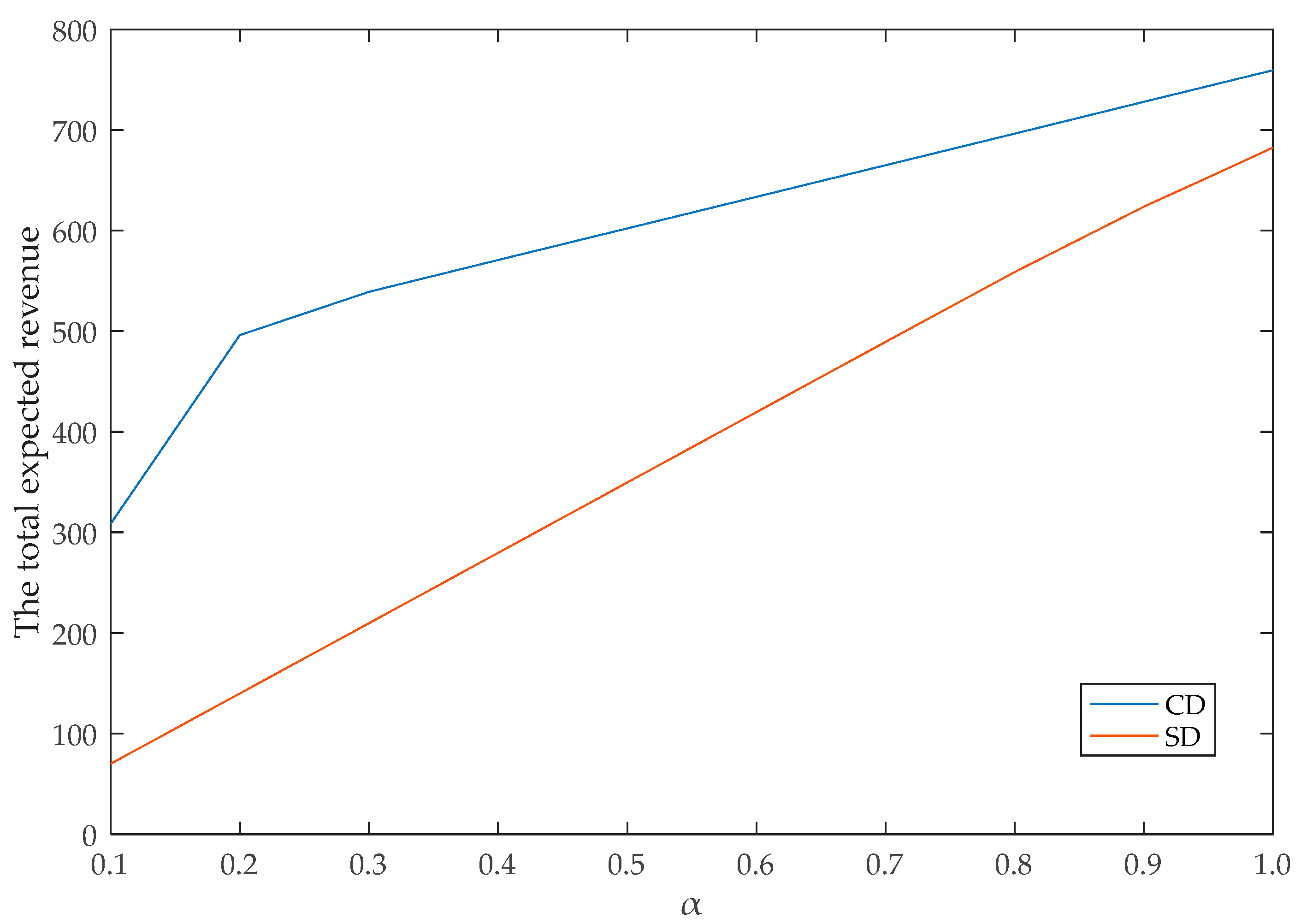
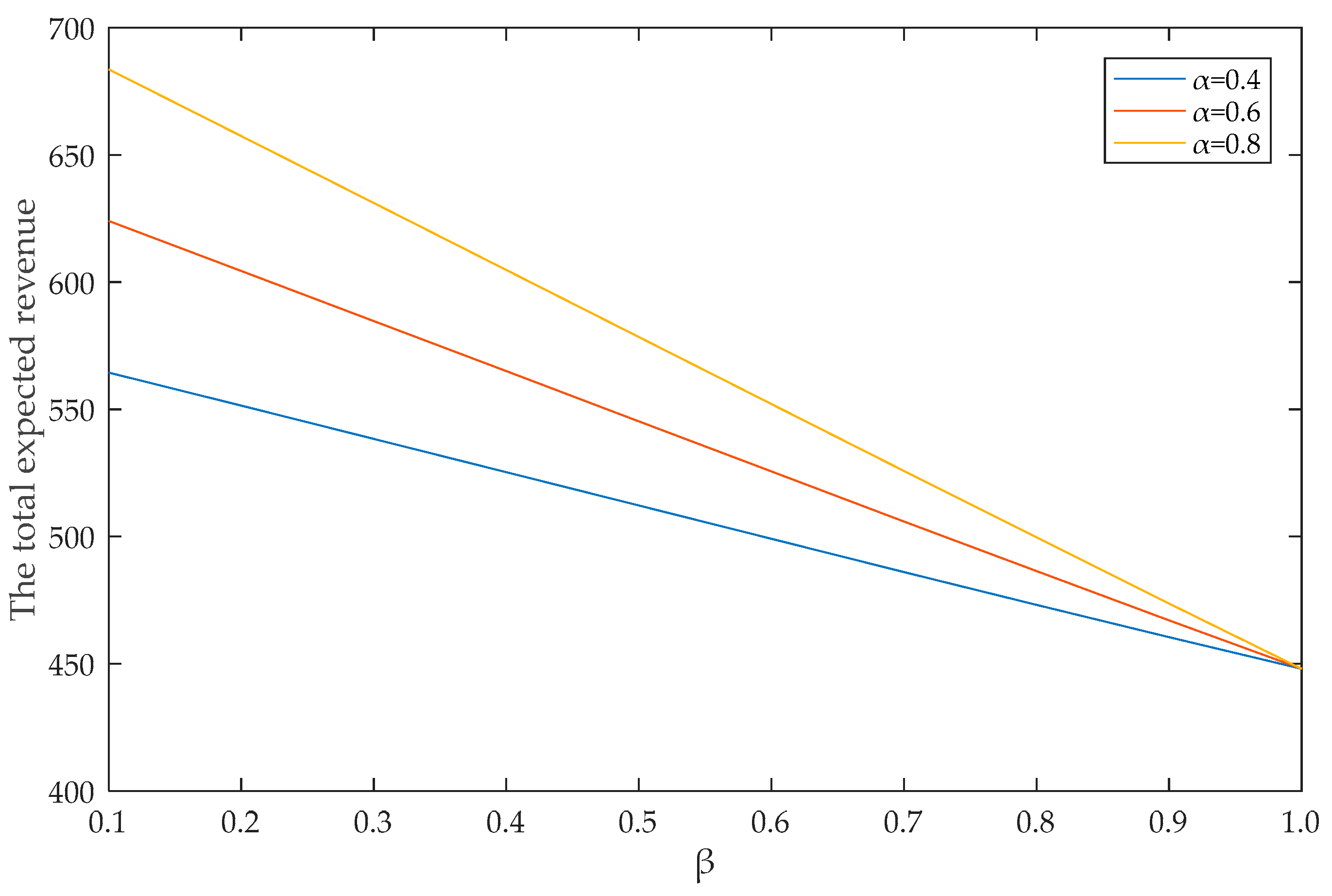
We investigated how group discounts affect total revenue when dynamic pricing is applied for individuals. The way of discounting group tickets can effectively stimulate group demand, and the booking of group discount tickets needs to be limited to maximize total revenue. Numerical experiments showed that decision making is superior to simple dynamic pricing when demand is weak.

(3)

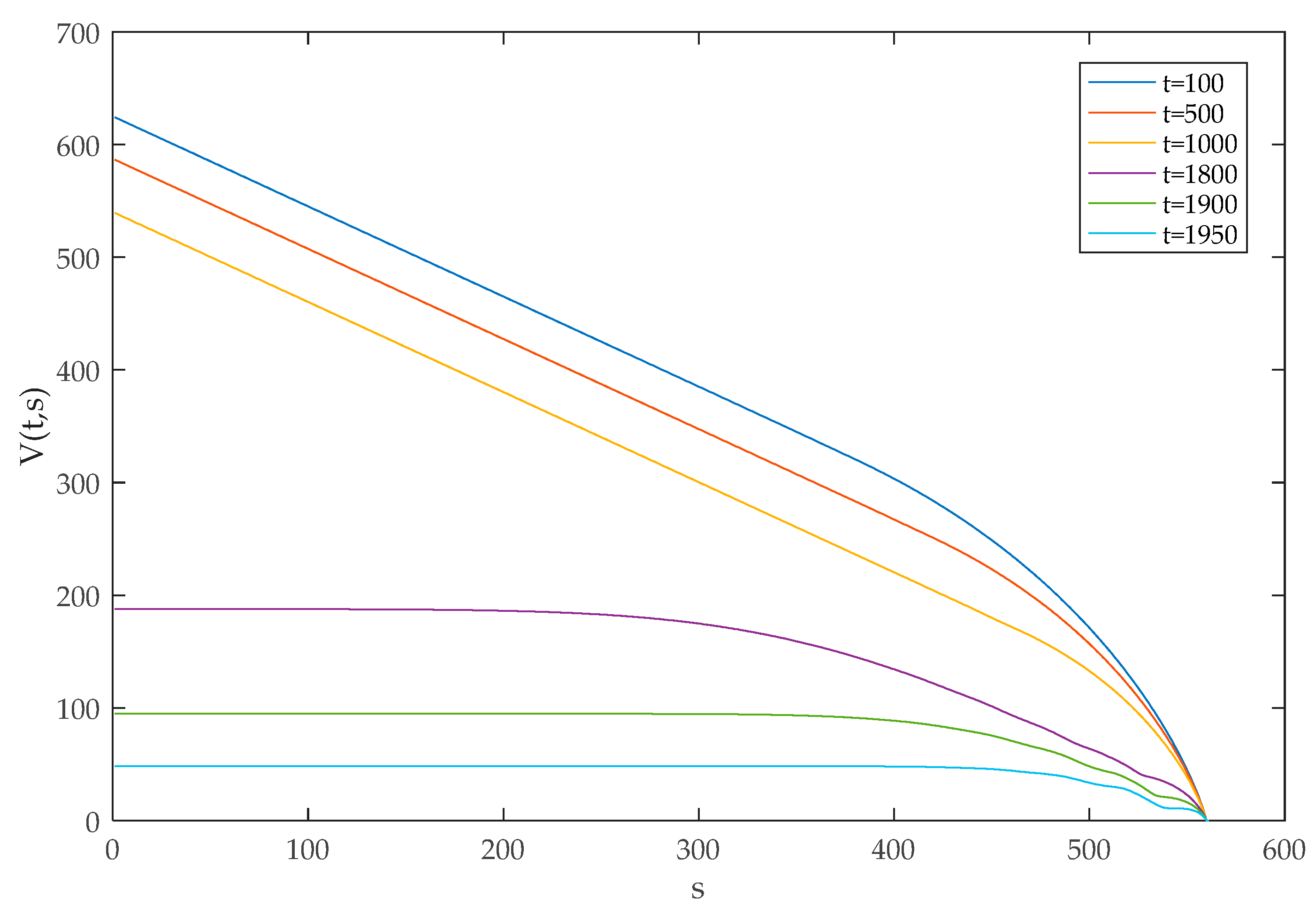
We investigated the effects of time and the sales volume of tickets on total revenue, and the effects of group demand and total demand on the total expected revenue. These rules will help rail operators to apply the comprehensive policy appropriately.

3. Methodology

In this section, we describe the problem and introduce the control process of joint decision making. The assumptions of building the model are elaborated on as well. Then, a dynamic programming model for the joint decision is proposed and the boundary conditions are given. Finally, the optimal policy is determined and the inverse recursive algorithm for solving the model is designed.

3.1. Problem Description

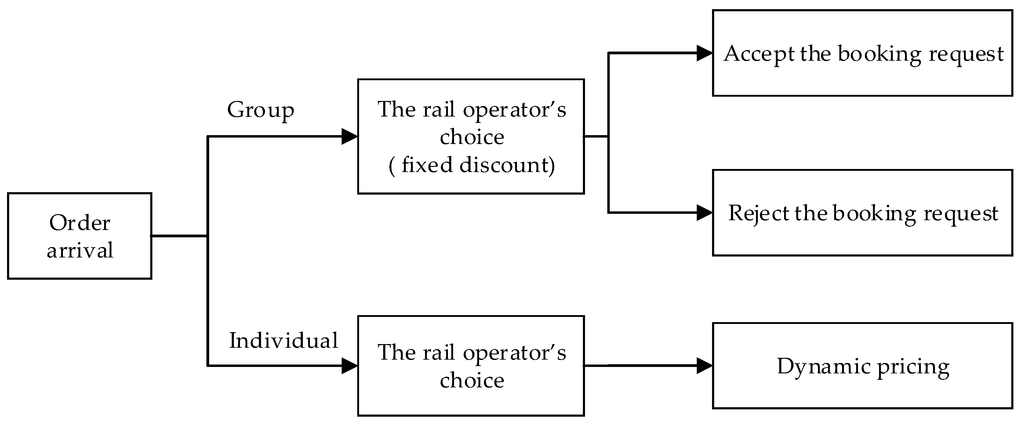
There is a train with $C$ second-class seats running between 2 stations. Because of the large volume of second-class seats, they are more appropriate for group booking and joint decision making. Here we studied a single-leg problem, so the number of tickets is equal to the number of seats. Tickets are sold before the train departs. Let the presale period be T. In order to improve revenue, the operator provides discount tickets for groups and applies dynamic pricing for individuals. Here we define that a group should include at least 20 passengers, which is in line with the regulations of the China Railway Corporation. Actually, the following proposed model can be adjusted for groups of any size based on the number of passengers. Therefore, arrival orders can be divided into 2 types: Group and individual orders. For group orders, operators provide a fixed discounts and limit the booking according to the number of tickets sold. For individual orders, operators decide on ticket prices dynamically and passengers buy tickets with a certain probability. The control process is shown in Figure 1.

The problem to be solved and its background are described now in detail. We divided the time interval $\left[0,T\right]$ finely enough so that at most, one order arrives in each period. Let $t$ be the time periods after sales begin. Sales begin at $t=0$ and end after $t=T$. The arrival orders fall into 2 categories: Group orders and individual orders. The average order arrival probability with one period is $\alpha$. The probability of the arriving order belonging to group orders is $\beta$. At any time, if the arriving order is a group order, passengers will only choose to purchase discounted tickets provided by the rail operator. It should be noted that the discount is fixed throughout the sales period, and the price for the group is denoted by $\theta$. To maximize the total revenue, railway operators should reserve appropriate seats for individual passengers at higher fares. Therefore, railway operators should limit the number of group purchases. If the arrival order is an individual one, the passenger purchases a ticket with a certain probability, according to the fare set by the rail operator. The purchase probability is related to the passenger reserve price. The fare will be dynamically adjusted based on time and number of seats sold. It was assumed that the reserve price of individuals (denoted as $x$) is independently and identically distributed, and the cumulative distribution function and probability density function are $F_t\left(x\right)$ and $f_t\left(x\right)$, respectively, which are continuously differentiable. For the sake of discussion, we assumed that $F_t\left(x\right)$ is strictly increasing. The reserve price is private information for the passengers, but information of $F_t\left(x\right)$ and $f_t\left(x\right)$ is symmetrical between the railway operator and the passenger.

This study was also based on the following assumptions:

(1)

The minimum price of dynamic pricing for individual orders is not less than the discount price for group orders, so as to ensure that groups will be attracted by the discount.

(2)

The order arrival rate is time homogeneous. In fact, although rail operators cannot predict demand accurately, they can estimate the average order arrival probability and the average proportion of group purchase orders in total orders based on historical data, so that we can consider the arrival probability of each type of order as time homogeneous.

(3)

The reserve price distribution information is symmetrical for the rail operator and passengers.

(4)

Overbooking, no-shows, refunds, and standing-room-only tickets were not considered.

3.2. Dynamic Programming Model for Joint Decision

3.2.1. Notation

For convenience, the notations are listed as follows:

$t$	Time periods after sale begins,$t\in \left[0,T\right]$; ticket presale begins at $t=0$ and ends after $t=T$
$\alpha$	Average order arrival probability within one period, $0<\alpha <1$
$\beta$	Probability of the arriving order belonging to group order, $0<\beta <1$${\alpha }_1$ Average arrival probability of group order within one period, ${\alpha }_1= \alpha \cdot \beta$
${\alpha }_2$	Average arrival probability of individual order within one period, ${\alpha }_2=\alpha \cdot (1-\beta )$
$\theta$	Discounted price for group
$x$	Reserve price for individuals
$F_t\left(x\right)$	Cumulative distribution function of $x$
$f_t\left(x\right)$	Density function of $x$
$y$	Number of passengers included in a group order
$P_j$	Probability of a group order including $j$ passengers
$s$	Number of tickets sold at the initiation of any interval
$C$	Total seats or tickets
$V\left(t,s\right)$	Value function, indicating expected revenue
$r\left(t,s\right)$	Dynamic fare for individuals (abbreviated as $r$ later)

3.2.2. Value Functions

Before constructing the recursive value function, 2 probabilities should be explained: The probability of passengers included in a group order, and the purchasing probability of an individual passenger.

For $j=1,2,\dots$, the probability of a group order including $j$ passengers is expressed as $P_j$, which can be estimated by historical data.

Let $s$ be the number of tickets sold at the initiation of any interval, and then the number of remaining tickets is $C-s$. $V\left(t,s\right)$ represents the total expected revenue from the beginning of time period $t$ to the end of ticket presale, when the number of tickets sold is $s$ at the beginning of $t$. $r\left(t,s\right)$ denotes the fare decided for individual orders by the rail operator in time period $t$ when the number of tickets sold is $s$ (abbreviated as $r$ later).

$F_t\left(x\right)$ is common knowledge for the rail operator and passengers. In period $t$, the number of sold tickets is $s$. When $r\left(t,s\right)$ is less than the reserved price for individuals, the ticket will be purchased. Therefore, the purchasing probability of the individual order is:

$$E_x\left[P\left(x\ge r\left(t,s\right)\right)\right]=1-F_t\left(r\left(t,s\right)\right)$$

(1)

To build the dynamic programming model, the following 2 situations must be considered separately:

(1) If $C-s\ge 20$, the number of remaining tickets is enough for a group, so the total expected revenue is shown as follows:

$$\begin{array}{ll}V\left(t,s\right)& ={\displaystyle {\sum }_{j=20}^{C-s}{\alpha }_1\times P_j}\times \max \left\{V\left(t+1,s\right),V\left(t+1,s+j\right)+\theta \times j\right\}\\ & +{\alpha }_1\left(1-{\displaystyle {\sum }_{j=20}^{C-s}{P}_j}\right)V\left(t+1,s\right)\\ & +{\alpha }_2\times \underset{r}{\max }\left\{\left(1-F_t\left(r\right)\right)\left(V\left(t+1,s+1\right)+r\right)+F_t\left(r\right)V\left(t+1,s\right)\right\}\\ & +\left(1-{\alpha }_1-{\alpha }_2\right)V\left(t+1,s\right)\end{array}$$

(2)

In order to facilitate the follow-up proof of theorems, we divided the expected revenue $V\left(t,s\right)$ into 3 parts to explain it. First, when the group order arrives, the railway operator decides whether to accept the order. When $20\le j\le C-s$, there are enough remaining tickets for the group. Let $H_1\left(t,s\right)$ denote the expected revenue of a group order as follows:

$$H_1\left(t,s\right)={\displaystyle {\sum }_{j=20}^{C-s}{\alpha }_1\times P_j}\times \max \left\{V\left(t+1,s\right),V\left(t+1,s+j\right)+\theta \times j\right\}$$

(3)

Second, when an individual order arrives, the railway operator decides the optimal price dynamically to maximize revenue. Let $H_2\left(t,s\right)$ denote the expected revenue of an individual order as follows:

$$H_2\left(t,s\right)={\alpha }_2\times \underset{r}{\max }\left\{\left(1-F_t\left(r\right)\right)\left(V\left(t+1,s+1\right)+r\right)+F_t\left(r\right)V\left(t+1,s\right)\right\}$$

(4)

Finally, when no order arrives within an interval, the number of tickets sold remains unchanged. The expected revenue is shown as the first part of $H_3\left(t,s\right)$. Similarly, when $j>C-s$, there are not enough remaining tickets for this group, the order cannot be accepted at this time. The expected revenue is thus shown as the remaining part of $H_3\left(t,s\right)$:

$$H_3\left(t,s\right)=\left(1-{\alpha }_1-{\alpha }_2\right)V\left(t+1,s\right)+{\alpha }_1\left(1-{\displaystyle {\sum }_{j=20}^{C-s}{P}_j}\right)V\left(t+1,s\right)$$

(5)

(2) If $C-s<20$, there are not enough remaining tickets for a group. Thus, the tickets can only be purchased by individuals. In fact, if the number of remaining tickets is insufficient, and the group wants to travel together, they will leave without purchasing any tickets. The total expected revenue is shown as follows:

$$\begin{array}{cc}V\left(t,s\right)& ={\alpha }_2\times \underset{r}{\max }\left\{\left(1-F_t\left(r\right)\right)\left(V\left(t+1,s+1\right)+r\right)+F_t\left(r\right)V\left(t+1,s\right)\right\}\\ & +\left(1-{\alpha }_2\right)V\left(t+1,s\right)\end{array}$$

(6)

3.2.3. Boundary Conditions

For the value functions of both situations above, the boundary conditions are identical and are shown as follows:

• $V\left(T+1,s\right)=0$, $\forall s$ indicates that the ticket’s residual value should be zero at the departure time of the train; and
• $V\left(t,C\right)=0$, $\forall t$ indicates that when tickets are sold out at the beginning of time period $t$, the expected revenue from time period t to T should be zero.

3.3. Optimal Policy

There are 2 policies to be decided in this problem: Booking limits for group orders and optimal prices for individuals. According to Theorem 1, the optimal price for individual orders can be obtained.

Theorem 1.

If${\left(1-F_t\left(r^{}\right)\right)}^2/f_t\left(r\right)$is a decreasing function of$r$, then the optimal price for individual orders satisfies

$$r_t^{*}-{\left(1-F_t\left(r^{*}\right)\right)}^2/f_t\left(r^{\ast }\right)=V\left(t+1,s\right)-V\left(t+1,s+1\right)$$

(7)

Proof. 

When $C-s\ge 20$, let the first derivative of $V\left(t,s\right)$ to $r$ be zero according to Equation (2):

$$\frac{\partial V\left(t,s\right)}{\partial r}={\alpha }_1\left[-f_t\left(r\right)\left(V\left(t+1,s+1\right)+r_t\right)+1-F_t\left(r\right)+f_t\left(r\right)V\left(t+1,s\right)\right]=0$$

Thus:

$$r_t-{\left(1-F_t\left(r\right)\right)}^2/f_t\left(r\right)=V\left(t+1,s\right)-V\left(t+1,s+1\right)$$

(8)

Let the second derivative of $V\left(t,s\right)$ to $r$ be:

$$\frac{{\partial }^{2}V\left(t,s\right)}{\partial r^2}={\alpha }_1\left[-f_t^{’}\left(r\right)\left(V\left(t+1,s+1\right)+r_t-V\left(t+1,s\right)\right)-2f_t\left(r\right)\right]$$

(9)

Substitute Equation (8) into Equation (9), then ${\partial }^{2}V\left(t,s\right)/\partial r^2={\alpha }_1\left[-f_t^{’}\left(r\right)\left(1-F_t\left(r\right)\right)/f_t\left(r\right)-2f_t\left(r\right)\right].$

Because ${\left(1-F_t\left(r\right)\right)}^2/f_t\left(r\right)$ is a subtraction function of $r$, ${\left[{\left(1-F_t\left(r\right)\right)}^2/f_t\left(r\right)\right]}^{’}=-1-F_t\left(r\right)/f_t\left(r\right)\ast f_t^{’}\left(r\right)\left(1-F_t\left(r\right)\right)-2f_t^2\left(r\right)/f_t\left(r\right)<0$. Thus, $-f_t^{’}\left(r\right)\left(1-F_t\left(r\right)\right)-2f_t^2\left(r\right)/f_t\left(r\right)<0$.

Therefore, ${\partial }^{2}V\left(t,s\right)/\partial r^2<0$. It is proven that Equation (3) has a unique optimal solution.

Similarly, we can prove that Equation (7) has a unique optimal solution and $r_t-{\left(1-F_t\left(r\right)\right)}^2/f_t\left(r\right)=V\left(t+1,s\right)-V\left(t+1,s+1\right)$ when $C-s<20$. □

Theorem 1 shows that the optimal price in Equation (7) corresponds to the optimal solution of the univariate programming problem. The optimal solution satisfies Equation (7). The conditions in Theorem 1 are easy to meet by most of the common distribution functions. When the reserved price distribution of passengers does not meet the conditions in Theorem 1, the one-dimensional search method can be used to solve the model.

As for the reservation limit of group tickets, since the gradient of value function with respect to $s$ is not monotonous, the group reservation limit varies with changes of $s$, $t$, and $j$. Therefore, let $u\in \left[0,1\right]$ be the control decision of group booking; when the group order is rejected $u=0$, otherwise $u=1$. The booking limit for group orders is dependent on Equation (10).

$$u\left(t,s,j\right)=\{\begin{array}{c}0,V\left(t+1,s\right)>V\left(t+1,s+j\right)+\theta \times j\\ 1,V\left(t+1,s\right)\le V\left(t+1,s+j\right)+\theta \times j\end{array}$$

(10)

3.4. Inverse Recursive Algorithm

Using Theorem 1 and the boundary conditions, the inverse recursive algorithm is designed to solve the model, shown as Algorithm 1. Combined with Theorem 1, the joint decision can be obtained.

Algorithm 1 Inverse recursive algorithm

1: Initialize $\forall s,V\left(T+1,s\right)=0$, and $\forall t,V\left(t,C\right)=0$

2: for $t=T$ to 1 do

3:  for $s=C-1$ to 1 do

4:   calculate $r\left(t,s\right)$ according to (7)

5:   If $\left(C-s\right)<20$, then

6:    calculate $V\left(t,s\right)$ according to (6)

7:   else

8:    calculate $V\left(t,s\right)$ according to (2)

9:   end if

10:  end for

11: end for

3.5. Application Process for the Rail Operator

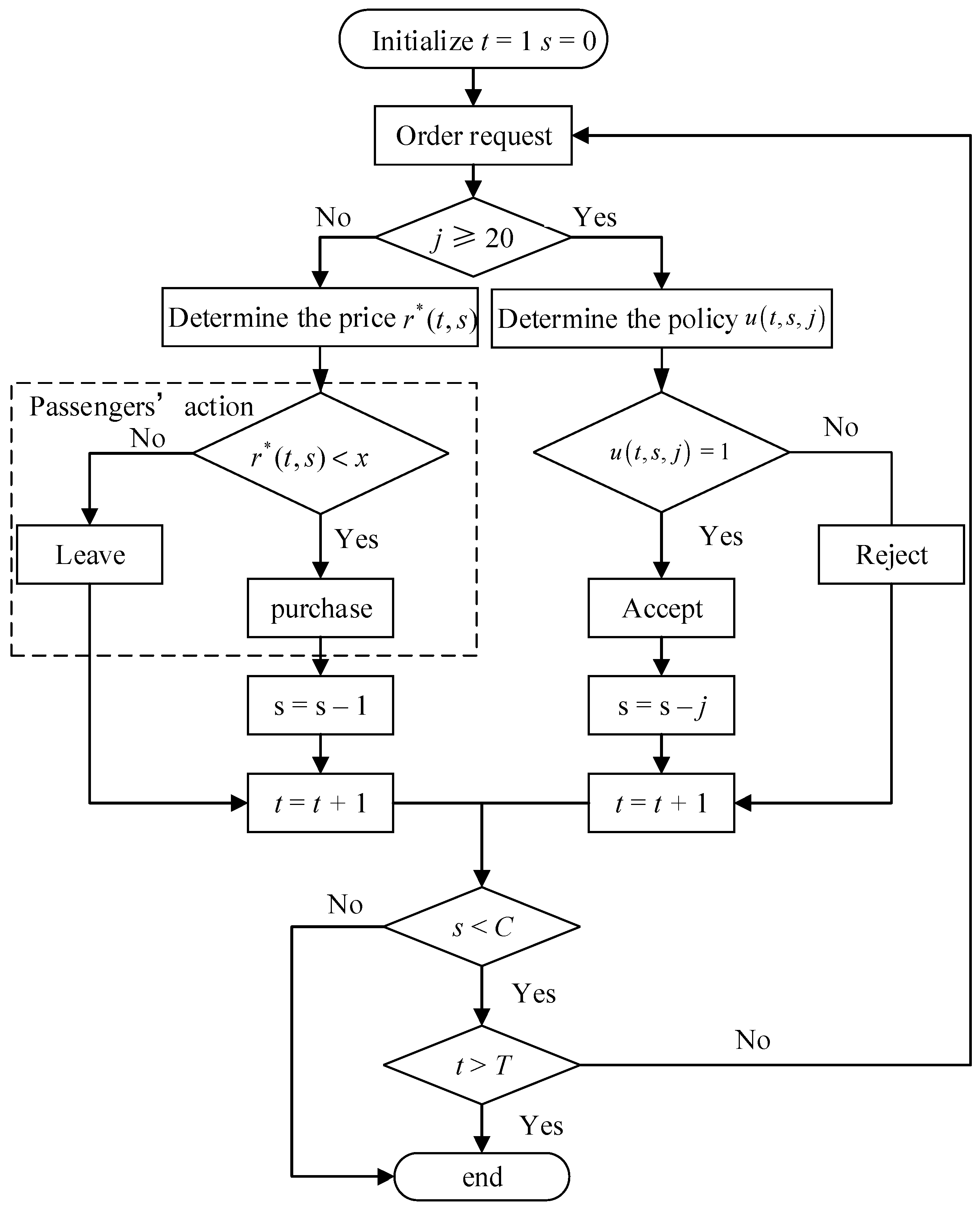
According to the above discussion, the rail operator can obtain the joint decision of group booking limits and the optimal price for individual passengers, based on the demand forecast. In the operation, the rail operator could apply the joint policy following the application process shown in Figure 2. At the beginning of $t$, for any $j$ (number of passengers in arriving order), the rail operator can obtain $r_t^{*}$ and $u\left(t,s,j\right)$, where $r_t^{*}$ is solved by Equation (8) or by one-dimensional search, $u\left(t,s,j\right)$ can be obtained by Equation (10). If an individual order arrives, the rail operator will provide price $r_t^{*}$; if a group order arrives, the rail operator makes a decision according to $u\left(t,s,j\right)$. If $u\left(t,s,j\right)=1$, the rail operator accepts the group order; otherwise, the group order will be rejected.

4. Numerical Experiments

In this section, numerical experiments verified the superiority and some other properties of joint decision making.

4.1. Data

The presale period is divided into 2000 periods, and at most, one order arrives at each period, so $T=2000$. The total arrival probability is represented by $\alpha$, where $\alpha =0.6$. Here $\alpha ={\alpha }_1+{\alpha }_2$. Let ${\alpha }_1=\beta \alpha$, so ${\alpha }_2=\left(1-\beta \right)\alpha$. $\beta$ represents the ratio of group orders to total orders and $\beta =0.2$. Assuming that there are 560 second-class seats in the electric multiple unit (abbreviated as EMU) with 8 vehicles, $C=560$. According to the Beijing Railway Administration, the number of passengers in a group order is generally between 20 and 40. Therefore, let the number of passengers in a group order follow a uniform distribution of [20, 40]. In this paper, it is assumed that the reserved price distribution of individual passengers is a static exponential distribution function $f(x)=1/\mu \times e^{-x/\mu }$ [15]; $\mu$ indicates the average price that passengers are willing to pay. We normalized the ticket fare, so that $\mu =1$, and the discount price for the group is set as $\theta =0.8$.

4.2. Results and Discussion

We used MATLAB R2016a to implement the algorithm on a desktop computer with 8.00 GB of memory, Intel(R) Core (TM) I5-7200u, and CPU 2.50 GHZ. The run time was 19.362 s. In order to verify the superiority of the model, the comprehensive model of group booking limits and dynamic pricing for individual passengers (CD) was compared with the simple dynamic pricing model without group discounts (SD) and dynamic pricing with fixed inventory for groups (DF).

4.2.1. Comparison between CD and SD

When $\alpha$ changes from 0.1 to 1, the expected total revenues of CD and SD change, as shown in Figure 3. It is shown that the expected revenue of CD is higher than that of SD, but with an increased order arrival probability, the gap between CD and SD gradually narrows. Thus, we changed $C$ to be among 100, 200, and 300 and kept other parameters unchanged. The total expected revenues of CD and SD are shown in

Table 1. Total expected revenue of CD and SD.

$\mathit{\alpha }$	C = 100		C = 200		C = 300
	CD	SD	CD	SD	CD	SD
0.1	58.89	104.02	58.89	184.02	58.89	264.02
0.2	114.89	130.45	117.78	210.50	117.78	290.50
0.3	154.61	156.58	176.64	236.98	176.67	316.98
0.4	183.12	182.27	231.07	263.45	235.56	343.45
0.5	205.31	204.22	275.10	289.93	294.08	369.93
0.6	223.47	222.20	311.31	316.35	347.36	396.41
0.7	238.84	237.42	342.00	342.36	393.15	422.89
0.8	252.16	250.60	368.61	367.81	432.98	449.37
0.9	263.91	262.24	392.10	391.13	468.17	475.83
1.0	274.43	272.65	413.13	412.04	499.68	502.20

. The values in bold in Table 1 indicate that SD is superior to CD. In order to obtain the superior threshold of CD, we defined the individual demand–supply ratio $\pi =T\cdot \alpha (1-\beta )/C$. By changing T to change $\pi$ and keeping other parameters unchanged, we obtained the expected total revenue from the experiment, as shown in

Table 2. Total expected revenue of CD and SD with changing π.

π	SD	CD
0.6	474.95	123.72
1.2	556.32	247.44
1.8	611.82	370.94
2.4	667.41	494.66
3.0	722.91	613.77
3.6	778.50	715.16
4.2	833.99	801.04
4.8	889.58	875.65
5.4	945.05	941.39
6.0	1000.15	1000.32
6.6	1052.72	1053.55
7.2	1101.27	1102.24

. When the individual demand–supply ratio reaches or exceeds 6.0, the expected revenue of SD is a little higher than that of DC. This is because the group discount is set lower than the individual price. Although the mechanism of CD allows a dynamic adjustment threshold for group orders, when individual demand is high enough, the benefit for not setting up group discounts is greater. However, when the individual demand–supply ratio is less than 6.0, group ticket discounts can effectively stimulate group demand and increase overall revenue.

To investigate how the interaction of $\alpha$ and $\beta$ affects the comparison of CD vs. SD, we conducted a simulation. The difference between the expected total revenue of CD and SD when $\alpha$ is 0.4, 0.6, and 0.8 is shown in Figure 4 and

Table 3. Difference between total expected revenue of CD and SD.

β	α = 0.4			α = 0.6			α = 0.8
	SD	CD-SD	%	SD	CD-SD	%	SD	CD-SD	%
0.01	291.51	181.80	62.37	437.26	185.86	42.50	581.55	123.99	21.32
0.02	288.56	271.45	94.07	432.84	206.33	47.67	575.97	128.24	22.26
0.03	285.62	286.90	100.45	428.43	209.04	48.79	570.35	131.35	23.03
0.04	282.67	289.32	102.35	424.01	211.58	49.90	564.68	134.47	23.81
0.05	279.73	291.05	104.05	419.59	214.09	51.02	558.98	137.61	24.62
0.06	276.78	292.74	105.77	415.18	216.59	52.17	553.23	140.77	25.44
0.07	273.84	294.42	107.52	410.76	219.07	53.33	547.45	143.95	26.29
0.08	270.89	296.09	109.30	406.34	221.55	54.52	541.65	147.16	27.17
0.09	267.95	297.76	111.12	401.93	224.03	55.74	535.81	150.39	28.07
0.10	265.01	299.42	112.99	397.51	226.50	56.98	529.96	153.63	28.99

. It can be seen that the smaller $\alpha$ is, the more obvious the advantages of CD are, and the larger $\beta$ is, the more obvious the advantages of CD are.

4.2.2. Comparison between CD and DF

Let $\gamma$ be the booking limits of group tickets in the DF model. For example, when $\gamma =100$, there are only 100 tickets for group orders. When all 100 tickets are sold to groups at the discount price, the operators will no longer accept group orders. At the same time, there are not enough group tickets remaining to meet the demand for arriving group orders, and group orders will be rejected. The operators apply the dynamic pricing policy for individuals throughout the presale period. The expected revenues of CD and DF when $\gamma$ changes from 0 to 500 are shown in Figure 5. The expected revenue of CD is better than that of DF at any time. Thus, it is necessary to dynamically adjust booking limits for group orders.

4.2.3. Impact of Proportion of Group Orders on Total Expected Revenue

Keeping the other parameters unchanged, we simulated the expected returns under different $\alpha$ and $\beta$, and got the results shown in

Table 4. Total expected revenue under different $\alpha$ and $\beta$.

β	α = 0.4	α = 0.6	α = 0.8
0.05	570.78	633.68	696.58
0.06	569.53	631.76	694.00
0.07	568.26	629.83	691.41
0.08	566.99	627.90	688.81
0.09	565.71	625.95	686.20
0.10	564.42	624.01	683.59

and Figure 6. It can be seen that with increased $\beta$ under the same $\alpha$, the total expected return decreases. This is because group discounts are lower than individual prices. Specifically, the higher the proportion of group demand, the smaller the expected revenue. When the proportion of group demand is small, railway companies use pricing to guide more individual demand to maximize revenue.

4.2.4. Law of Change of Value Function

The variation of $V\left(t,s\right)$ with $t$ and $s$ is shown in Figure 7. When the value of $s$ is fixed, the expected revenue $V\left(t,s\right)$ decreases as the value of $t$ increases. Thus, the nearer the departure time, the lower the expected revenue of remaining tickets for the railway company. The impact of $s$ on $V\left(t,s\right)$ is also shown in Figure 8. For most time periods, when the value of $t$ is fixed, the expected revenue $V\left(t,s\right)$ decreases with increased $s$, and the marginal benefit of tickets $\Delta V\left(t,s\right)=V\left(t,s\right)-V\left(t,s+1\right)$ increases as the number of tickets sold increases. However, when the presale comes to the end, the expected revenue $V\left(t,s\right)$ of the railway company is not the decreasing convex function of $s$.

5. Conclusions

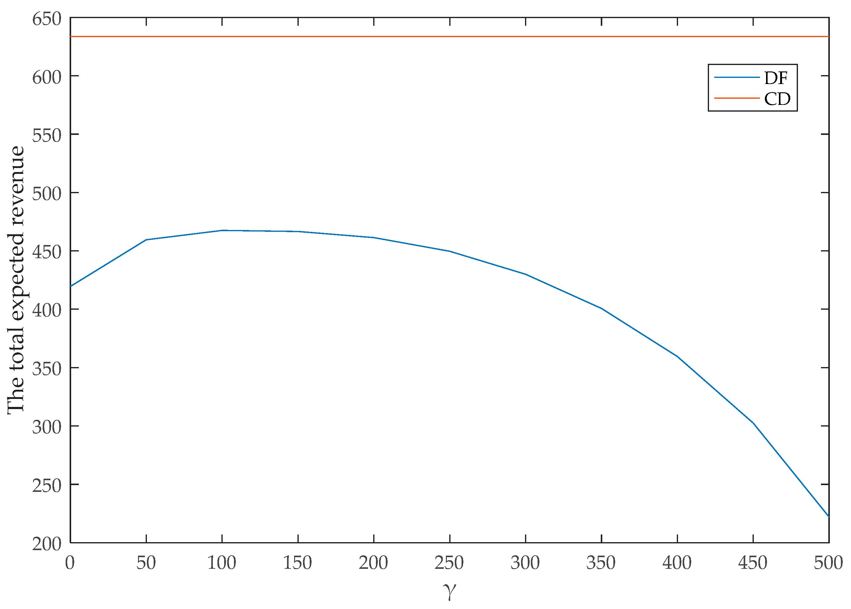
In this study, we used dynamic programming to model the joint decision of inventory control and dynamic pricing considering group reservations and designed a reverse recursive algorithm to obtain a control policy. For group reservations, the operators provide discounts and decide on booking limits, while applying dynamic pricing for individual reservations. The main contribution of this study is that the effect of group discounts on dynamic pricing was investigated and the proposed model enriches the theory of joint decision making. Numerical experiments show that the proposed joint policy is superior to the dynamic pricing policy without groups in terms of expected revenue when individual demand is weak, and it is always superior to the dynamic policy with a fixed group inventory. Thus, if group discounts are integrated into the dynamic pricing policy, the inventory of groups needs to be controlled dynamically to maximize the expected revenue.

This study shows the advantage of incorporating group discounts into dynamic pricing. The network problem of multiple trains and multiple stops, considering competitive factors and nonhomogeneous, constrained information, will be the future research direction. Future study also could introduce local or national conditions and investigate the financial effects, such as the cost of providing cards for unemployed people or people with large families.