Utilization of the Brinkman Penalization to Represent Geometries in a High-Order Discontinuous Galerkin Scheme on Octree Meshes

Abstract

We investigate the suitability of the Brinkman penalization method in the context of a high-order discontinuous Galerkin scheme to represent wall boundaries in compressible flow simulations. To evaluate the accuracy of the wall model in the numerical scheme, we use setups with symmetric reflections at the wall. High-order approximations are attractive as they require few degrees of freedom to represent smooth solutions. Low memory requirements are an essential property on modern computing systems with limited memory bandwidth and capability. The high-order discretization is especially useful to represent long traveling waves, due to their small dissipation and dispersion errors. An application where this is important is the direct simulation of aeroacoustic phenomena arising from the fluid motion around obstacles. A significant problem for high-order methods is the proper definition of wall boundary conditions. The description of surfaces needs to match the discretization scheme. One option to achieve a high-order boundary description is to deform elements at the boundary into curved elements. However, creating such curved elements is delicate and prone to numerical instabilities. Immersed boundaries offer an alternative that does not require a modification of the mesh. The Brinkman penalization is such a scheme that allows us to maintain cubical elements and thereby the utilization of efficient numerical algorithms exploiting symmetry properties of the multi-dimensional basis functions. We explain the Brinkman penalization method and its application in our open-source implementation of the discontinuous Galerkin scheme, Ateles. The core of this presentation is the investigation of various penalization parameters. While we investigate the fundamental properties with one-dimensional setups, a two-dimensional reflection of an acoustic pulse at a cylinder shows how the presented method can accurately represent curved walls and maintains the symmetry of the resulting wave patterns.

1. Introduction

In simulations of fluid motion for engineering scenarios, we generally need to deal with obstacles or containment of a non-trivial shape. In mesh-based schemes, we have two options to represent such geometries: we can try to align the mesh with the geometries, such that the walls build a boundary of the mesh or we try to embed the boundary conditions inside the mesh elements. The first option eases the formulation of boundary conditions and their treatment in the scheme [1]. The second option avoids the need to adapt the mesh to the, possibly complex, geometry [2]. Correctly aligning the mesh with arbitrary geometries in the first option can become cumbersome for high-order approximations. Thus, the embedding method is attractive for high-order schemes. Another application area, where the embedded boundaries provide a benefit, are moving geometries, as the need for new meshes can be avoided during simulations.

High-order discretization schemes can represent smooth solutions with few degrees of freedom. This is an essential property for algorithms on modern computing systems as the memory bandwidth is a strongly limiting factor on new systems, due to the widening memory gap. A numerical scheme that allows for high-order approximations of the solution is the discontinuous Galerkin finite element method. In this method, the solution within elements is represented by a function series (usually a polynomial series). In this work, we are concerned with a high-order discontinuous Galerkin scheme and the embedded geometry representation within it. Besides the possibility to use high-order approximations, the discontinuous Galerkin scheme also offers a relatively loose coupling between elements, resulting in a high computational locality, which in turn is advantageous for modern parallel computing systems. Discontinuous Galerkin methods are, therefore, increasingly popular and relevant.

Peskins [3] was one of the first scientists trying to impose immersed boundaries for his investigations. For his studies, he simulated the flow around heart valves considering the incompressible Navier–Stokes equations while introducing the immersed boundaries, using an elastic model and applying forces to the fluid, thus changing the momentum equations. His work was extended by Saiki and Biringen [4], and they considered feedback forces for the immersed boundaries to represent a rigid body while using an explicit time-stepping, hence resulting in stiff problems and very small time-stepping for the simulation. An important fact, which makes immersed boundary methods more attractive, is the introduction of the effect of the geometry in the governing equations themselves. Embedding the boundaries in the mesh relaxes the requirements on the elements, and using simple elements allows for efficient numerical algorithms that can, for example, exploit inherent symmetric properties of the discretization. The additionally introduced terms can either be considered in the numerical discretization or the continuous equations. Applying forcing terms in the discretization allows for better control of the numerical accuracy and the conservation properties of the used discretization method; on the other hand, the generality and flexibility of these methods disappear when considering different solvers using different discretization methods. In contrast, the volume penalization method imposes additional forcing penalty terms on the continuous equations, while the discretization is done as usual [5]. The Brinkman Penalization Method (BPM) is one of these methods. It was originally developed by Arquis and Caltagirone [6] for numerical simulations of isothermal obstacles in incompressible flows. The idea is to model the obstacle as a porous material, with material properties approaching zero. The major benefit of this method is error estimation, which can be rigorously predicted in terms of the penalization parameters [7]. Furthermore, the boundary conditions can be enforced to a precision, without changing the numerical discretization of the scheme. Kevlahan and Ghidaglia already applied this method for incompressible flows, while considering a non-moving, as well as a moving geometry. They used a pseudo-spectral method [8] in their works.

Liu and Vasilyev employed the volume penalization for the compressible Navier–Stokes equations. In their publication [9], they discussed a 1D and a 2D test case. They used a wavelet method for the discretization and showed error convergence and resulting pressure perturbations for acoustic setups. In other investigations, various numerical discretization methods were used, which showed promising results using the Brinkman penalization method. In [10,11], the pseudo-spectral methods, in [9], wavelet, and in [12], the finite volume/finite element methods were used. However, as far as we know, no work on this kind of penalization in the context of high-order discontinuous Galerkin methods for compressible Navier–Stokes equations has been done so far. Thus, this paper will look into the Brinkman penalization employed within a high-order discontinuous Galerkin solver. Our implementation is available in our open-source solver Ateles [13].

2. Numerical Method

The flow of compressible viscous fluids can mathematically be described by the Navier–Stokes equations governing the conservation of mass, momentum, and energy. In this section, we describe the compressible Navier–Stokes equation with the Brinkman penalization method to model solid obstacles as proposed in [9]. We apply this penalization in the frame of the Discontinuous Galerkin (DG) method and introduce this method also briefly in this section. The additional source terms introduced by the penalization increase the stiffness of the scheme considerably, and the last part of this section discusses how this can be overcome by an implicit-explicit time integration scheme.

2.1. The Compressible Navier–Stokes Equation

The Navier–Stokes equations describe the motion of fluids and model the conservation of mass, momentum, and energy. The non-dimensional compressible equations in conservative form can be written as:

$$\frac{\partial \rho }{\partial t}=-\nabla ·\mathbf{m},$$

(1)

$$\frac{\partial m_i}{\partial t}+\sum _{j=1}^3\frac{\partial }{\partial x_j}\left(m_i{v}_j+p{\delta }_{ij}\right)-\frac{1}{Re}\sum _{j=1}^3\frac{\partial }{\partial x_j}{\tau }_{ij}=0i=1,2,3$$

(2)

$$\frac{\partial \rho e}{\partial t}+\nabla ·\left[\left(e+\frac{p}{\rho }\right)\mathbf{m}\right]-\frac{1}{Re}\sum _{j=1}^2\frac{\partial }{\partial x_j}\left(\sum _{i=1}^2{\tau }_{ij}{v}_i-\frac{1}{\gamma -1}\frac{\mu }{Pr}T\right)=0$$

(3)

where the conserved quantities are the density $\rho$, the momentum $\mathbf{m}=\rho \mathbf{v}$, and the total energy density e, given by the sum of kinetic and internal energy density:

$$e=\frac{1}{2}{\left|\mathbf{v}\right|}^2+\frac{p}{\rho (\gamma -1)}.$$

(4)

where $\mathbf{v}={(v_1,v_2,v_3)}^T$ is the velocity vector, ${\delta }_{ij}$ is the Kronecker delta, $Re$ is the reference Reynolds number, and $Pr$ the reference Prandtl number. $\gamma$ stands for the isentropic expansion factor, given by the heat capacity ratio of the fluid, and T denotes the temperature. Viscous effects are described by the shear stress tensor:

$${\tau }_{ij}=\mu \left(\frac{\partial v_i}{\partial x_j}+\frac{\partial v_j}{\partial x_i}\right)$$

(5)

and the dynamic viscosity $\mu$.

To close the system, we use the ideal gas law as the equation of state, which yields the following relation:

$$p=\rho RT.$$

(6)

where R represents the gas constant.

2.2. The Brinkman Penalization

Penalization schemes employ additional, artificial terms to the equations in regions where the flow is to be inhibited (penalized). In the conservation of momentum and energy, we can make use of local source terms that penalize deviations from the desired state. With the Brinkman penalization, we also inhibit mass flow through obstacles by introducing the Brinkman porosity model and using a low porosity, where obstacles are to be found. Extending the compressible Navier–Stokes equations from Section 2.1 by the penalization terms, we obtain Equations (7) and (9).

$$\begin{array}{cc}\hfill \frac{\partial \rho }{\partial t}& =-\nabla ·\left[1+\left(\frac{1}{\varphi }-1\right)\chi \right]\mathbf{m},\hfill \\ \hfill \frac{\partial m_i}{\partial t}+\sum _{j=1}^3\frac{\partial }{\partial x_j}\left(m_i{v}_j+p{\delta }_{ij}\right)-\frac{1}{Re}\sum _{j=1}^2\frac{\partial }{\partial x_j}{\tau }_{ij}\end{array}$$

(7)

$$\begin{array}{cc}\hfill & =-\frac{\chi }{\eta }\left(v_i-U_{oi}\right)i=1,2,3,\hfill \\ \hfill \frac{\partial \rho e}{\partial t}+\nabla ·\left[\left(e+\frac{p}{\rho }\right)\mathbf{m}\right]-\frac{1}{Re}\sum _{j=1}^2\frac{\partial }{\partial x_j}\left(\sum _{i=1}^2{\tau }_{ij}{v}_i-\frac{1}{\gamma -1}\frac{\mu }{Pr}T\right)\end{array}$$

(8)

$$\begin{array}{cc}\hfill & =-\frac{\chi }{{\eta }_T}\left(T-T_o\right).\hfill \end{array}$$

(9)

The obstacle has the porosity $\varphi$, the velocity $U_o$, and the temperature $T_o$. The strength of the source terms can be adjusted by the viscous permeability $\eta$ and the thermal permeability ${\eta }_T$. The masking function $\chi$ describes the geometry of obstacles and is zero outside of obstacles and one inside. It is also referred to as the characteristic function. It is capable of dealing not only with complex geometries but also with variations in time.

$$\chi (\mathbf{x},t)=\left\{\begin{array}{cc}1,\hfill & \mathrm{if}x\in \mathrm{obstacle}.\hfill \\ 0,\hfill & \mathrm{otherwise}.\hfill \end{array}\right.$$

(10)

To represent a solid wall for compressible fluids properly, Liu et al. [9] stated that the porosity $\varphi$ should be as small as possible, i.e., $0<\varphi <<1$. They scaled the permeabilities with the porosity and introduced according scaling factors $\alpha$ and ${\alpha }_T$. The permeabilities were then defined by $\eta =\alpha \varphi$ and ${\eta }_T={\alpha }_T\varphi$. With these relations, Liu et al. [9] found a modeling error of $O({\eta }^{1/2}\varphi )$ for resolved boundary layers in the material and $O({(\eta /{\eta }_T)}^{1/4}{\varphi }^{3/4})$ for non-resolved boundary layers. In both cases, the error was dominated by the porosity. Nevertheless, the error can still be minimized with sufficiently small viscous permeabilities $\eta$.

Moreover, small values of the porosity caused stability issues and imposed a heavy time-step restriction with our numerical scheme. With the introduction of $\varphi$, the eigenvalues of the hyperbolic system changed, which has adverse effects on stability. The eigenvalues of the system of equations along with penalization terms [9] are given by the following characteristic equation:

$$-{(\lambda -u)}^3+\left[c^2+\frac{u^2}{2}({\varphi }^{-1}-1)(\gamma -3)\right](\lambda -u)-c^{2}u({\varphi }^{-1}-1)(\gamma -1)=0,$$

(11)

where $c={(\gamma p/\rho )}^{1/2}$ and $\gamma$, p, $\rho$, and u are the ratio of specific heat, pressure, density, and velocity, respectively. For $\varphi =1$, the system of equations yields three eigenvalues $u,u+c,u-c,$ which implies the speed of sound c in the medium, which is what we would like to achieve. However, with $0<\varphi <<1$, the eigenvalues can no longer be evaluated easily and are linked to $\varphi$, which causes problems for the hyperbolic part.

2.3. The Discontinuous Galerkin Discretization

In this section, we briefly introduce the semi-discrete form of the Discontinuous Galerkin finite element method (DG) for compressible inviscid flows. The compressible Euler equations were derived from the Navier–Stokes equations by neglecting diffusive terms. They still provide a model for the conservation of mass, momentum, and energy in the fluid and can be described in vectorial notation by:

$${\partial }_t\mathbf{u}+\nabla ·\mathbf{F}\left(\mathbf{u}\right)=0,$$

(12)

equipped with suitable initial and boundary conditions. Here, $\mathbf{u}$ is a vector of the conservative variables, and the flux function $\mathbf{F}\left(\mathbf{u}\right)={(\mathbf{f}\left(\mathbf{u}\right),\mathbf{g}\left(\mathbf{u}\right))}^T$ for two spatial dimensions is given by:

$$\mathbf{u}=\left[\begin{array}{c}\rho \\ \rho u\\ \rho v\\ \rho E\end{array}\right],\mathbf{f}\left(\mathbf{u}\right)=\left[\begin{array}{c}\rho u\\ \rho u^2+p\\ \rho uv\\ (\rho E+p)u\end{array}\right],\mathbf{g}\left(\mathbf{u}\right)=\left[\begin{array}{c}\rho v\\ \rho uv\\ \rho v^2+p\\ (\rho E+p)v\end{array}\right],$$

where $\rho ,\mathbf{v}={(u,v)}^T,E,p$ denotes the density, velocity vector, specific total energy, and pressure, respectively. The system is closed by the equation of state assuming the fluid obeys the ideal gas law with pressure defined as $p=(\gamma -1)\rho \left(e-\frac{1}{2}(u^2+v^2)\right)$; where $\gamma =\frac{c_p}{c_v}$ is the ratio of specific heat capacities and e is the total internal energy per unit mass.

The discontinuous Galerkin formulation of the above equation was obtained by multiplying it with a test function $\psi$ and integrating it over the domain $\Omega$. Thereafter, integration by parts was used to obtain the following weak formulation:

$${\int }_{\Omega }\psi \frac{\partial \mathbf{u}}{\partial t}d\Omega +{\oint }_{\partial \Omega }\psi \mathbf{F}\left(\mathbf{u}\right)·\mathbf{n}ds-{\int }_{\Omega }\nabla \psi ·\mathbf{F}\left(\mathbf{u}\right)d\Omega =0,\forall \psi ,$$

(13)

where $ds$ denotes the surface integral. A discrete analogue of the above equation was obtained by considering a tessellation of the domain $\Omega$ into n closed, non-overlapping elements given by $T=\left\{{\Omega }_i\right|i=1,2,\dots ,n\}$, such that $\Omega ={\cup }_{i=1}^n{\Omega }_i$ and ${\Omega }_i\cap {\Omega }_j=\varnothing \forall i\ne j$. We define a finite element space consisting of discontinuous polynomial functions of degree $m\ge 0$ given by:

$$P^m=\{f\in {\left[L^2(\Omega )\right]}^m:f_{|{\Omega }_k}\in {\mathbb{P}}^m\left({\Omega }_k\right)\forall {\Omega }_k\in \Omega \}$$

(14)

where ${\mathbb{P}}^m\left({\Omega }_k\right)$ is the space of polynomials with largest degree m on element ${\Omega }_k$. With the above definition, we can write the approximate solution ${\mathbf{u}}_h(\mathbf{x},t)$ within each element using a polynomial of degree m:

$${\mathbf{u}}_h(\mathbf{x},t)=\sum _{i=1}^m{\widehat{u}}_i{\varphi }_i,{\psi }_h\left(\mathbf{x}\right)=\sum _{i=1}^m{\widehat{v}}_i{\varphi }_i,$$

(15)

where the expansion coefficients ${\widehat{u}}_i$ and ${\widehat{v}}_i$ denote the degrees of freedom of the numerical solution and the test function, respectively. Notice that there is no global continuity requirement for ${\mathbf{u}}_h$ and ${\psi }_h$ in the previous definition. Splitting the integrals in Equation (13) into a sum of integrals over elements ${\Omega }_i$, we obtain the space-discrete variational formulation:

$$\sum _{i=1}^n\frac{\partial }{\partial t}{\int }_{{\Omega }_i}{\psi }_h{\mathbf{u}}_{h}d\Omega +{\oint }_{\partial {\Omega }_i}{\psi }_h\mathbf{F}\left({\mathbf{u}}_h\right)·\mathbf{n}ds-{\int }_{{\Omega }_i}\nabla {\psi }_h·\mathbf{F}\left({\mathbf{u}}_h\right)d\Omega =0,\forall {\psi }_h\in P^m.$$

(16)

Due to the element local support of the numerical representation, the flux term is not uniquely defined at the element interfaces. The flux function is, therefore, replaced by a numerical flux function ${\mathbf{F}}^{*}({\mathbf{u}}_h^{-},{\mathbf{u}}_h^{+},\mathbf{n})$, where ${\mathbf{u}}_h^{-}$ and ${\mathbf{u}}_h^{+}$ are the interior and exterior traces at the element face in the direction $\mathbf{n}$ normal to the interface. A choice of appropriate numerical flux can then be selected from several numerical flux schemes. For our simulations, we used the Lax–Friedrichs scheme for numerical flux.

For simplicity, we can re-write the equation above in matrix vector notation and obtain:

$$\frac{\partial }{\partial t}\widehat{\mathbf{u}}=M^{-1}\left(S·\mathbf{F}\left(\widehat{\mathbf{u}}\right)-M^F·\mathbf{F}\left(\widehat{\mathbf{u}}\right)\right)=:rhs\left(\widehat{\mathbf{u}}\right).$$

(17)

where M, S denote the mass and the stiffness matrices and $M^F$ are the so-called face mass lumping matrices. The above obtained ordinary differential Equation (17) can be solved in time using any standard time-stepping method, e.g., a Runge–Kutta method.

In our implementation, we exploited the fact that we only used cubical elements. This choice of simple elements allowed for a tensor-product notation in the multi-dimensional basis functions. The symmetry of the elements enabled efficient dimension-by-dimension algorithms in the computation.

2.4. The Implicit-Explicit Time Discretization

As the penalization introduces stiff terms to the equations and for accuracy, we would want them to be as stiff as possible, we introduce an implicit time integration for those terms. With an otherwise explicit time integration scheme, this results in an implicit-explicit time-stepping scheme that can be achieved by splitting the right-hand side of the equations into an explicitly integrated part and an implicitly integrated part. Therefore, to perform time integration of the system, we use a Diagonally Implicit Runge–Kutta (DIRK) scheme with three explicit and four implicit stages as presented in [14]. The following section first considers a single implicit Euler step, to discuss the arising equations that need to be solved in each implicit stage of the higher order time discretization.

We denote the right-hand side by Q and employ the superscript $\iota$ for the implicit part and the superscript $\xi$ for the explicit part. By using the conservative quantities as subscripts ($\rho$, m, and e), we can distinguish the right-hand sides for the different equations. Thus, we get:

$$\begin{array}{cc}\hfill \frac{\partial \rho }{\partial t}& =Q_{\rho }^{\xi }+Q_{\rho }^{\iota }\hfill \end{array}$$

(18)

$$\begin{array}{cc}\hfill \frac{\partial m_i}{\partial t}& =Q_{m_i}^{\xi }+Q_{m_i}^{\iota }\hfill \end{array}$$

(19)

$$\begin{array}{cc}\hfill \frac{\partial e}{\partial t}& =Q_e^{\xi }+Q_e^{\iota }\hfill \end{array}$$

(20)

and we chose the implicit parts as:

$$\begin{array}{cc}\hfill Q_{\rho }^{\iota }& =0\hfill \end{array}$$

(21)

$$\begin{array}{cc}\hfill Q_{m_i}^{\iota }& =-\frac{\chi }{\eta }\left(u_i-U_{oi}\right)\hfill \end{array}$$

(22)

$$\begin{array}{cc}\hfill Q_e^{\iota }& =-\frac{\chi }{{\eta }_T}\left(T-T_o\right)\hfill \end{array}$$

(23)

out of Equations (7) and (9).

This choice restricts the implicit computation to the local source terms, which can be evaluated pointwise. Unfortunately, the introduced Brinkman porosity in (7) affects the flux and introduces spatial dependencies. To avoid the need for the solution of an equation system across the whole domain for this dependency, the porosity part will be computed in the explicit time-stepping scheme.

Observation for the Implicit Part

Considering Equations (18)–(20) only with their implicit parts, we get the following equation system:

$$\begin{array}{cc}\hfill \frac{\partial \rho }{\partial t}& =0\hfill \end{array}$$

(24)

$$\begin{array}{cc}\hfill \frac{\partial m_i}{\partial t}& =-\frac{\chi }{\eta }\left(u_i-U_{oi}\right)\hfill \end{array}$$

(25)

$$\begin{array}{cc}\hfill \frac{\partial e}{\partial t}& =-\frac{\chi }{{\eta }_T}\left(T-T_o\right).\hfill \end{array}$$

(26)

Notice that these equations can be solved pointwise as no spatial derivatives appear.

A discretization of these equations in time with a Euler backward scheme yields the solvable equation system:

$$\begin{array}{cc}\hfill \frac{\rho (t+\Delta t)-\rho \left(t\right)}{\Delta t}& =0\hfill \end{array}$$

(27)

$$\begin{array}{cc}\hfill \frac{m_i(t+\Delta t)-m_i\left(t\right)}{\Delta t}& =-\frac{\chi }{\eta }\left(u_i(t+\Delta t)-U_{oi}\right)\hfill \end{array}$$

(28)

$$\begin{array}{cc}\hfill \frac{e(t+\Delta t)-e\left(t\right)}{\Delta t}& =-\frac{\chi }{{\eta }_T}\left(T(t+\Delta t)-T_o\right).\hfill \end{array}$$

(29)

Equation (27) trivially yields $\rho (t+\Delta t)=\rho \left(t\right)$. With the implied constant density, we can now solve the equation for the change in momentum (28) and arrive at an explicit expression for the velocity $u_i(t+\Delta t)$ at the next point in time:

$$\begin{array}{cc}\hfill \frac{\rho (t+\Delta t)u_i(t+\Delta t)-\rho \left(t\right)u_i\left(t\right)}{\Delta t}& =-\frac{\chi }{\eta }\left(u_i(t+\Delta t)-U_{oi}\right)\hfill \end{array}$$

(30)

$$\begin{array}{cc}\hfill u_i(t+\Delta t)& =\frac{\rho \left(t\right)u_i\left(t\right)+\frac{\chi \Delta t}{\eta }{U}_{oi}}{\rho \left(t\right)+\frac{\chi \Delta t}{\eta }}.\hfill \end{array}$$

(31)

Finally, density and velocity at the new point in time can be used to find the new temperature as well by substituting the above results in Equation (29) and solving for the temperature at the next point in time. We find:

$$T(t+\Delta t)=\frac{\frac{\chi \Delta t}{{\eta }_T}{T}_o+c_v\rho \left(t\right)T\left(t\right)+\frac{\rho \left(t\right)}{2}(u_i^2\left(t\right)-u_i^2(t+\Delta t))}{c_v\rho \left(t\right)+\frac{\chi \Delta t}{{\eta }_T}}.$$

(32)

where $u_i(t+\Delta t)$ is given by Equation (31).

Thus, this specific choice of terms for the implicit part of the time integration scheme yields a system that can be solved explicitly and without much additional computational effort. However, the implicit discretization allows for arbitrarily small values of $\eta$ and ${\eta }_T$. A similar approach was developed by Jens Zudrop to model perfectly electrical conducting boundaries in the Maxwell equations, and more details can also be found in his thesis [15].

To solve the complete system, we then employed the diagonally implicit Runge–Kutta scheme with three explicit stages and four implicit stages [14]. It provides a scheme that is third order in time and L-stable.

Note, that while this approach overcomes time step limitations with respect to the permeabilities $\eta$ and ${\eta }_T$, the porosity term changes the eigenvalues of the hyperbolic system and affects the stability.

3. Results and Discussion

To investigate the penalization scheme in our discontinuous Galerkin implementation, we first analyzed the fundamental behavior in two one-dimensional setups and then considered the scattering at a cylinder in a two-dimensional setup.

As explained in Section 2.2, the modeling error by the penalization for the compressible Navier–Stokes equations as found by Liu and Vasilyev [9] was expected to scale with the porosity $\varphi$ by an exponent between $3/4$ and one and with the viscous permeability $\eta$ by an exponent between $1/4$ and $1/2$. To achieve low errors, you may, therefore, be inclined to minimize $\varphi$. However, with the implicit mixed explicit time integration scheme presented in Section 2.4, we can eliminate the stiffness issues due to small permeabilities with little additional costs, while the stability limitation by the porosity persists. Because of this, we deem it more feasible to utilize a small viscous permeability instead of a small porosity. At the same time, the relation between viscous permeability $\eta$ and thermal permeability ${\eta }_T$ gets small without overly large ${\eta }_T$. Therefore, we used a slightly different scaling than proposed by Liu and Vasilyev [9]. We introduce the scaling parameter $\beta$ and define the permeabilities accordingly in relation to the porosity as follows.

$$\eta ={\beta }^2·{\varphi }^2$$

(33)

$${\eta }_T=0.4\beta ·\varphi$$

(34)

Note, that we then expect the modeling error to be of size $O\left({\beta }^{1/4}{\varphi }^{3/4}\right)$.

3.1. One-Dimensional Acoustic Wave Reflection

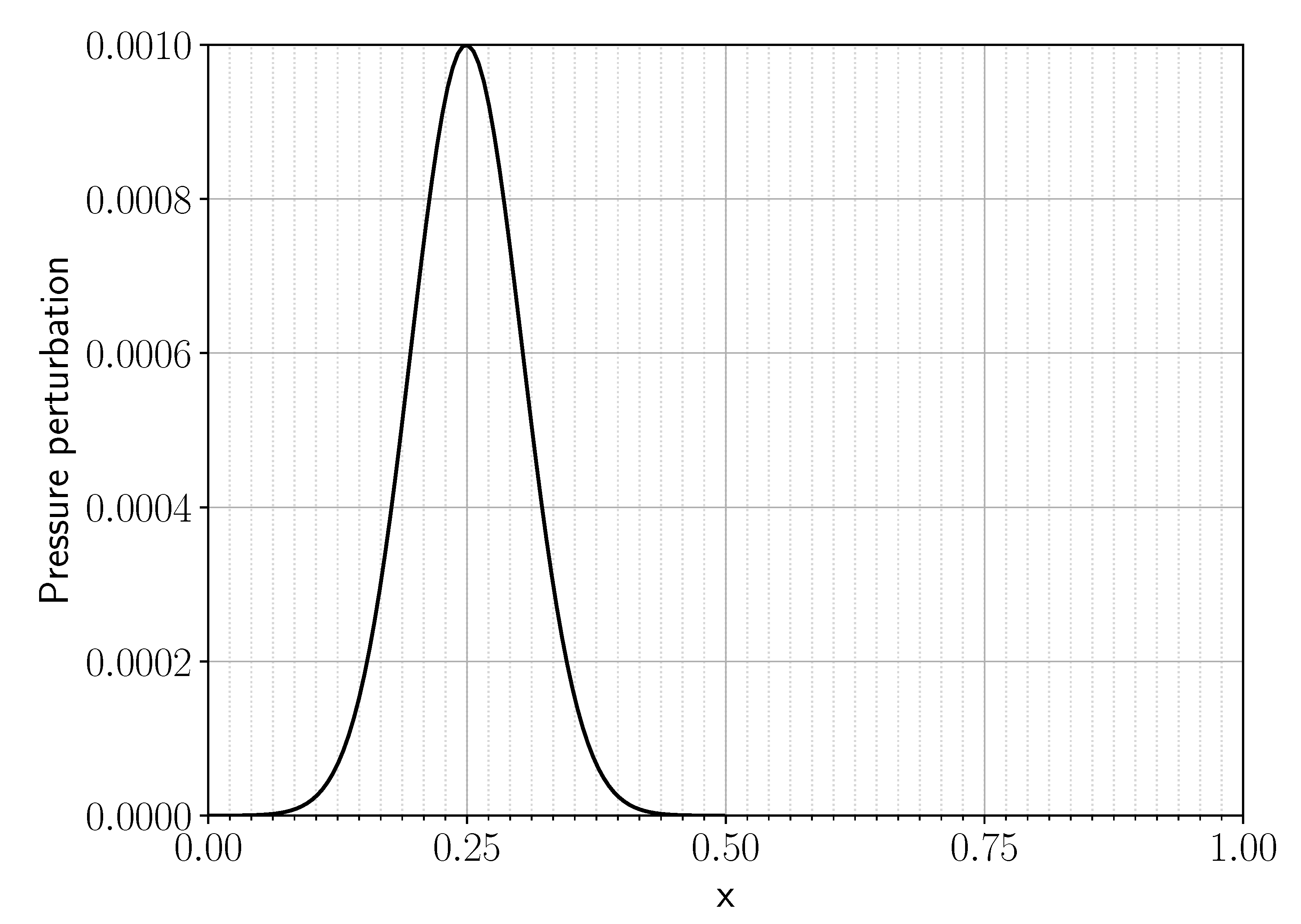
To assess how well the penalization scheme can capture the reflective nature of a solid wall, we used the reflection of an acoustic wave at the material. The initial pressure distribution is shown in Figure 1. It is described by the Gaussian pulse given in Equation (35) around its center at $x=0.25$ in the left half of the domain ($x\le 0.5$).

$${\rho }^{\prime }=u^{\prime }=p^{\prime }=ϵ\exp \left[-\ln \left(2\right)\frac{{(x-0.25)}^2}{0.004}\right]$$

(35)

For the amplitude $ϵ$ of the wave, we used a value of $ϵ={10}^{-3}$. The perturbations in density ${\rho }^{\prime }$, velocity $u^{\prime }$, and pressure $p^{\prime }$ from (35) are applied to a constant, non-dimensionalized state with a speed of sound of one. This results in the initial condition for the conservative variables density $\rho$, momentum m, and total energy e as described in: (36).

$$\rho =1+{\rho }^{\prime },m=\rho u^{\prime },e=\frac{1}{\gamma (\gamma -1)}+\frac{p^{\prime }}{\gamma -1}+\frac{1}{2}\rho {\left(u^{\prime }\right)}^2$$

(36)

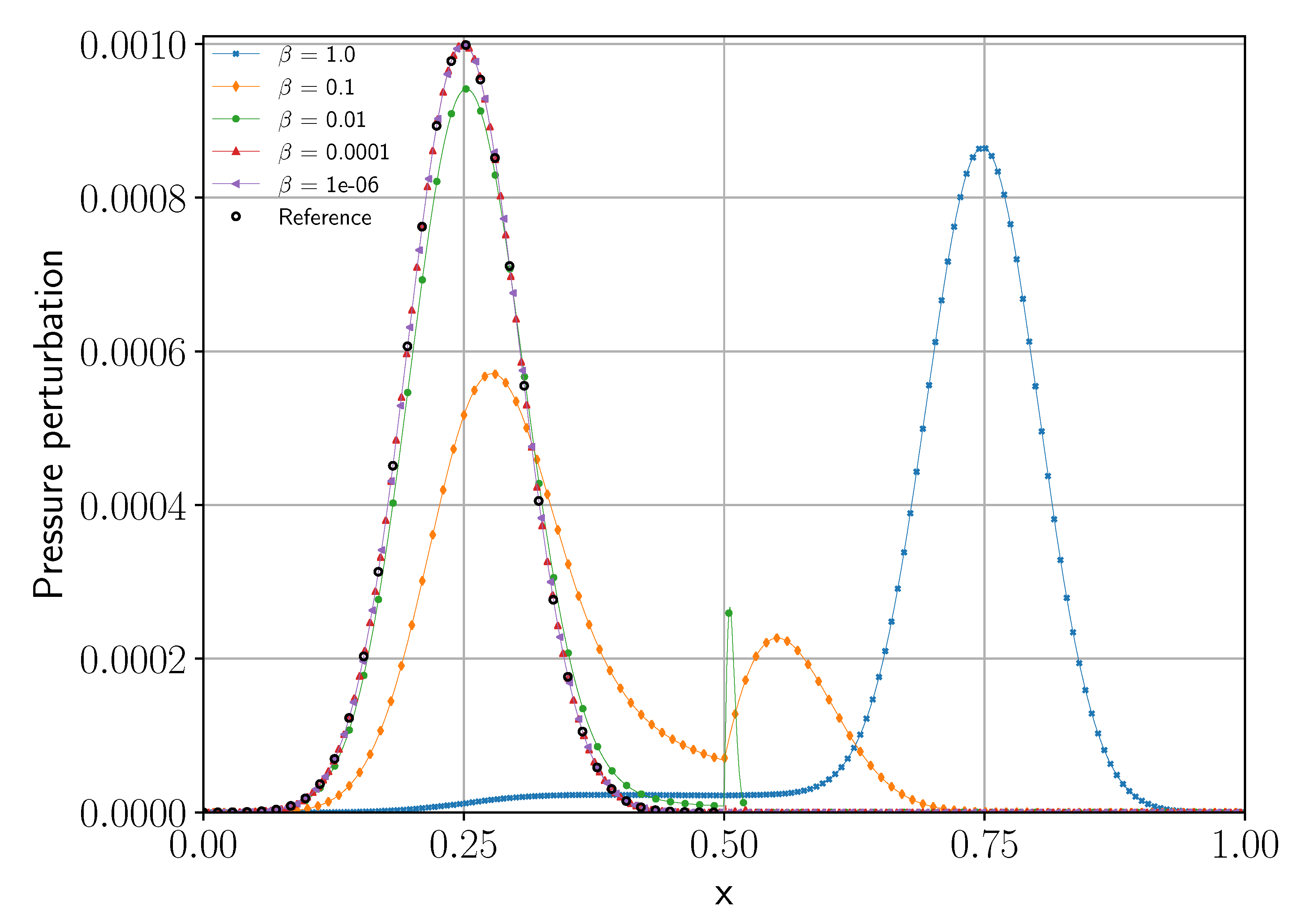
The penalization with porous medium is applied in the right half of the domain ($x>0.5$). In acoustic theory, the reflection should be perfectly symmetric, and the reflected pulse should have the same shape and size, only with opposite velocity. This simple setup allows us to analyze the dampening of the reflected wave and induced phase errors. Reflected waves for different settings of $\beta$ as defined in Equation (33) are shown in Figure 2. The pressure distribution for the reflection is shown for the state after a simulation time of $0.5$. With linear acoustic wave transport and a speed of sound of one, the pulse should return to its original starting point, just with an opposite traveling direction. This symmetry makes it easy to judge both the loss in wave amplitude and the phase shift of the reflected pulse.

While the analytical result for a linear wave transport provided a good reference in general for the acoustic wave, it sufficiently deviated from the nonlinear behavior to limit its suitability for convergence analysis to small error values. Therefore, we compared the simulations with the penalization method to numerical results with traditional wall boundary conditions and a high resolution. This reference was computed with the same element length, but the domain ended at $x=0.5$ with a wall boundary condition, and a maximal polynomial degree of 255 was used (256 degrees of freedom per element) to approximate the smooth solution. The resulting pressure profiles for different settings of $\beta$ and a fixed porosity of $\varphi =1.0$ are shown in Figure 2. This illustrates how well the wave was reflected for different settings of $\beta$ and that the solid wall reflection was well approximated for sufficiently small values of $\beta$. These numerical results were obtained with 48 elements and a maximal polynomial degree of 31 (32 degrees of freedom per element). Note that this setup aligns the wall interface with an element interface, where the discontinuity in the penalization is actually allowed by the numerical scheme. Later, we will discuss the changes observed, when moving the wall surface into the elements.

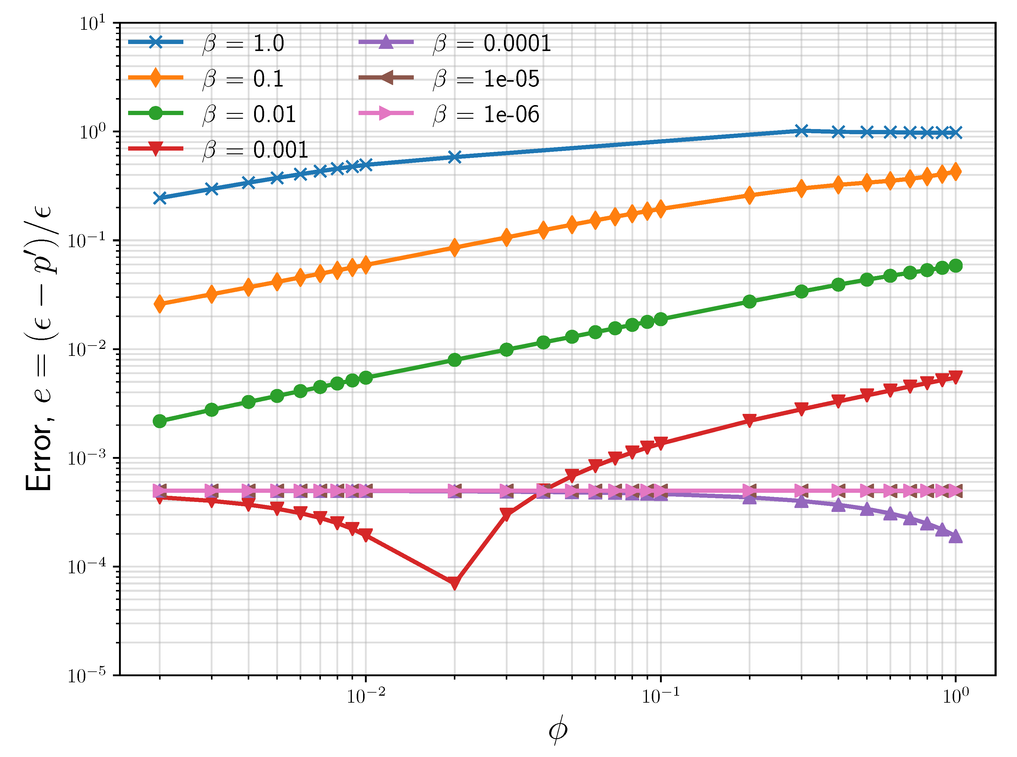
Figure 3 illustrates the impact of the porosity on the error in amplitude of the reflected wave for the same discretization with 48 elements and a maximal polynomial degree of 31. We plotted the error $e=(ϵ-p^{\prime }(t=0.5))/ϵ$ over porosity $\varphi$ for various scaling parameters of $\beta$ between one and ${10}^{-6}$. A scaling parameter of $\beta =1$ means that the error is only driven by the porosity $\varphi$, and for large values of $\beta \ge {10}^{-2}$, we observed the expected reduction in the error with decreasing porosity. However, with $\beta ={10}^{-3}$, this comes eventually to an end (no improvements for $\varphi <2\times {10}^{-2}$), and for smaller values of $\beta$, no improvements for the error can be achieved by lowering the porosity anymore. As can be seen in this figure, a sufficiently small permeability can yield the accuracy as a small porosity.

In Figure 3 as well, for $\beta =1e^{-3}$, we observed a drop in error, and then it increased again with smaller $\varphi$ to reach a convergence point finally. We would like to point out that this was expected to come from our numerical scheme using polynomials to represent the solution. Each data-point in the plot with varying $\varphi$ and $\beta$ represents a slightly different test case in terms of boundary layer thickness, as pointed out in Section 2.2. A sweet spot is reached when the degree of polynomial used for the simulation correctly captures the boundary layer in the problem. However, as we move further left from here, this sweet spot is slowly gone with further thinning of the boundary layer. With the same polynomial degree used, one would also expect to see this behavior for lines representing $\beta <1e^{-3}$ and correspondingly larger $\varphi$. This is exactly what we also see for $\beta =1e^{-4}$ and the value of $\varphi$ close to 1.0. For all other lines in the plot, this spot does not fall within the range of the figure.

By using the implicit mixed explicit scheme from Section 2.4, it is possible to exploit drastically smaller values for the permeabilities to cover up the lack of porosity in the penalization. On the other hand, the porosity cannot that easily be treated in our discretization, and even moderate values of $\varphi$ can have a dramatic impact on the time step restriction, due to the changed eigenvalues in the hyperbolic part of the equations.

Next, we performed a convergence analysis shifting the position of the wall such that it intersected the element at different locations. The reason for performing such an analysis becomes imperative when we consider the high-order numerical scheme used. We represented the solution state within an element using polynomials. For the pointwise evaluation of the nonlinear terms, we employed the Gaussian integration points, at which also the masking function of the penalization needs to be evaluated. Within an element, these integration points were scattered, being more concentrated on the element interface, and were rather sparse at the center. Therefore, in a peculiar validation test case like this one, when the wall was aligned with the element interface, due to the abundance of interpolation points, it had the advantage of being very precisely represented even for comparatively fewer degrees of freedom. In actual simulations, the wall interface may intersect an element at any point. We, therefore, also need to consider such intersections through the element and ensure the solution converges to the reference solution. The penalization method itself was not restrictive to any such limitations and could perfectly represent wall irrespective of its location within an element.

Thus, we performed and compared convergence analysis on two different discretizations, one where the wall lied at the element interface and a second where the wall intersected one element exactly in the middle. We would like to point out that the later scenario yielded a worst case estimate for the approximation of the jump in the masking function within an element. As explained, this simply came from scarce integration points lying around the center of element. For the following convergence analysis, we ignored the porosity (i.e., set $\varphi =1$) and used small permeabilities by choosing $\beta ={10}^{-6}$. We also considered the $L^2$ error norm now in the fluid domain. As a reference solution, we employed a numerical simulation with a traditional wall boundary and a high maximal polynomial degree of 255 (256 degrees of freedom per element). The error was measured at $t=0.5$ after the reflected wave reached its initial position again.

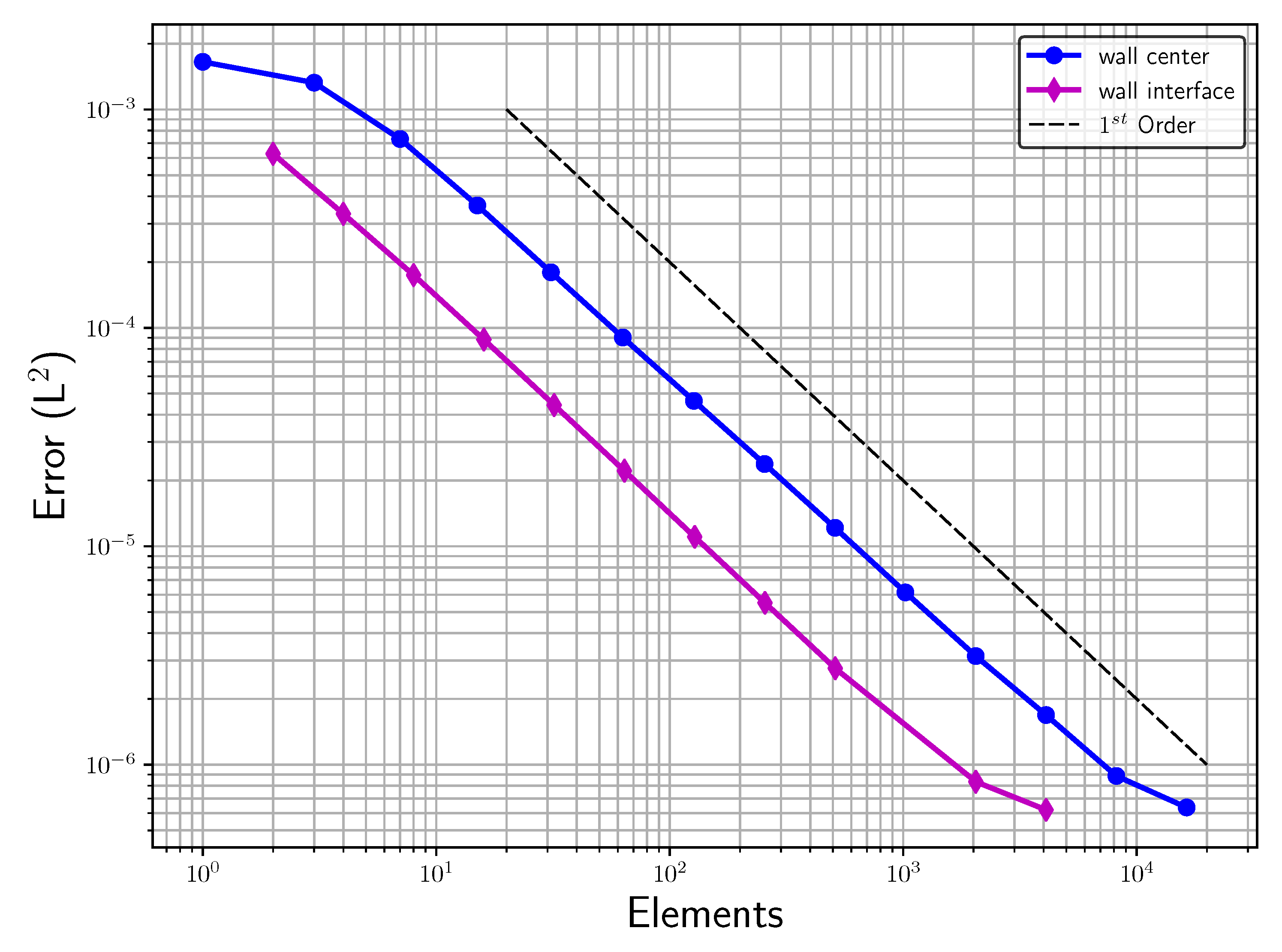
Figure 4 shows the $L^2$ norm of the error for the reflected pressure wave with a maximal polynomial degree of seven over an increasing number of elements (h-refinement). This plot compares the two discretizations explained. As expected, in Figure 4, we observe superior convergence behavior for the case when the wall lies at the element interface in comparison to the other case where the wall is crossing through the element center. However, for both cases, we observed a proper convergence towards the solution with a traditional solid wall boundary condition. The order of error convergence did not match the high-order discretization in either case, but this was expected due to the discontinuity introduced by the masking function of the penalization.

Next, we performed another convergence study using the same two discretizations, but this time keeping the number of elements constant and increasing the order of polynomial representation within those elements.

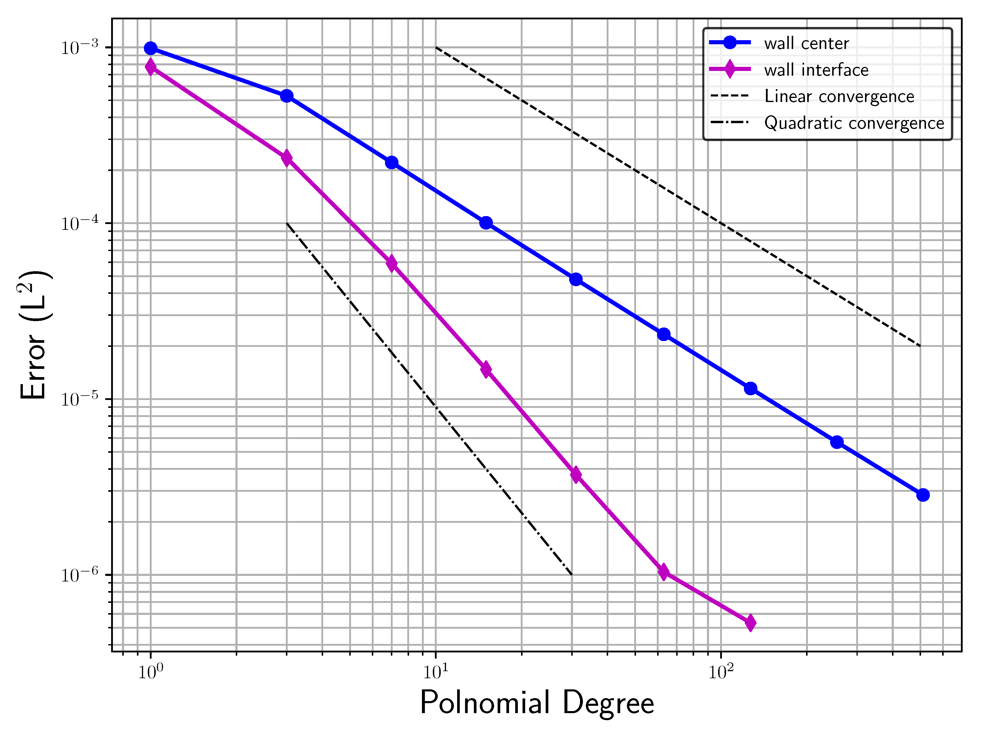
Figure 5 shows the error convergence over the maximal polynomial degree in the discretization scheme (p-refinement) with the number of elements fixed to 24. Here, also, one observes a solution in both cases converging to the reference solution. While no spectral convergence was achieved for the discontinuous problem, a quadratic convergence can be observed. This shows that a high-order approximation was beneficial even with the discontinuous masking function for the penalization.

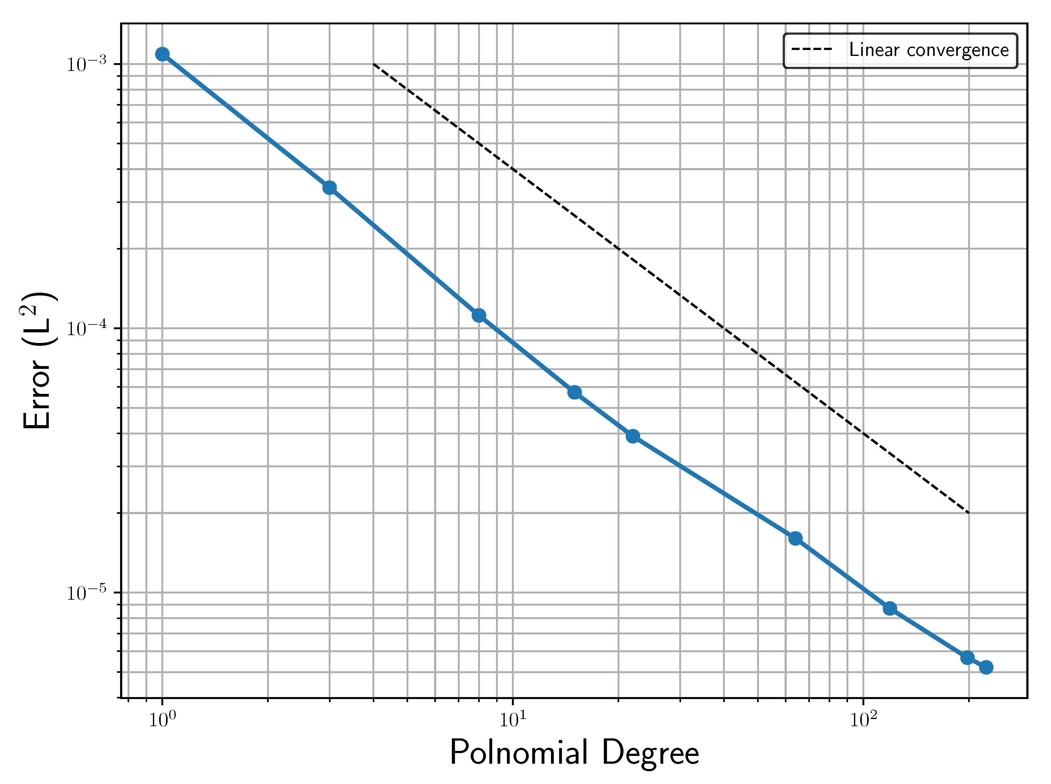
Finally, we also looked at the case where the wall was close to the element interface, but not exactly on it. This is a potential critical configuration for the numerical scheme being used, as the discontinuity close to the surface needs to be properly captured. We put the wall at 5% of the element length away from the element surface and measured the error as before, resulting in the graph shown in Figure 6. For this case as well, we observed a similar convergence rate as before, though the error was a little bit worse than with the wall on the interface.

For a smooth solution, the advantage of high-order methods to attain a numerical solution of a given quality using fewer degrees of freedom is well documented [16]. However, for a complex nonlinear problem with a discontinuity introduced by the porous medium, it is not so clear whether there is still a computational advantage by a high-order discretization. To investigate this, we ran the wall reflection problem for several orders and plotted the convergence with respect to the required computational effort, as seen in Figure 7. This test was performed starting with 16 elements in each data series, providing the leftmost point for the respective spatial scheme order. For subsequent data points, the number of elements was always increased by a factor of two up to the point where an error of ${10}^{-6}$ was achieved. 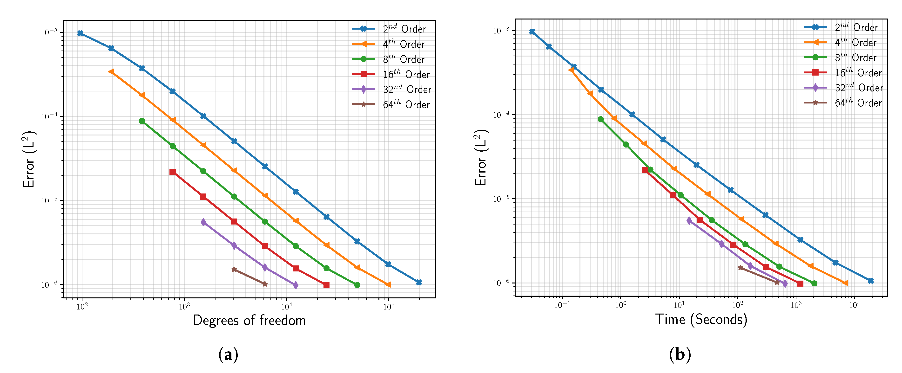Figure 7a depicts the observed $L^2$ error over the total number of degrees of freedom in the simulation. Here, we can see that for attaining a certain level of accuracy, the number of degrees of freedom required was always less when using a higher spatial order, even though the convergence rate did not increase with the scheme order. The high-order discretization, thus, allowed for memory-efficient computations, also in this case with a discontinuity present at the wall.

While for the memory consumption, there seems to be a clear benefit in high-order discretizations, it is not so clear whether this still holds for the required computing time. The time step limitation of the explicit scheme required more time steps for higher spatial scheme orders, increasing the computational effort to reach the desired simulation time. Additionally, the number of operations increased with higher orders due to the nonlinearity of the equations. Figure 7b shows the measured running times on a single computing node with 12 Intel Sandy-Bridge cores for the same runs. Again, the achieved accuracy is plotted, but this time over the observed running time in seconds. As can be seen, the advantage in terms of running times was not as clear as in terms of memory. However, we still observed faster times to the solution with higher spatial scheme orders, despite the increased number of time steps. In conclusion, we found some computational benefit from higher spatial scheme orders even in the presence of a discontinuity in this setup.

3.2. One-Dimensional Shock Reflection

After considering the reflection of an essentially linear acoustic wave, we now look into the reflection of a shock, where nonlinear terms play an important role. However, we neglected viscosity in this setup and only solved the inviscid Euler equations. The reflection of a one-dimensional shock wave at a wall was described and numerically investigated by Piquet et al. [17], for example. We used their setup to validate the penalization method in our discontinuous Galerkin setup, even though a high-order scheme is not ideal for the representation of shocks.

The downstream state in front of the shock (denoted by 1) is given in

Table 1. Shock state description.

Downstream speed of sound	$c_1$	1.0
Shock Mach number	$M{a}_s$	1.2
Shock velocity	$u_s$	1.2
Downstream density	${\rho }_1$	1.0
Downstream pressure	$p_1$	${\gamma }^{-1}$
Downstream velocity	$u_1$	0.0
Isentropic coefficient	$\gamma$	1.4

. The upstream state after the shock (denoted by 2) is then given by the Rankine–Hugoniot conditions for the shock Mach number $M{a}_s$. These yield:

$$\frac{{\rho }_2}{{\rho }_1}=\frac{\gamma +1}{\gamma -1+2{M{a}_s}^{-2}}$$

(37)

for the relation of densities $\rho$ in up- and downstream of the shock and

$$\frac{p_2}{p_1}=\frac{2\gamma {M{a}_s}^2-(\gamma -1)}{\gamma +1}$$

(38)

for the relation of pressures p.

With these relations, the ratio of the upstream ($p_3$) and downstream ($p_2$) pressure for the reflected shock wave is [18]:

$$\frac{p_3}{p_2}=\frac{M{a}_s^2(3\gamma -1)-2(\gamma -1)}{2+M{a}_s^2(\gamma -1)}$$

(39)

For the computation of the velocity $u_{rs}$ of the reflected shock wave, we considered Equation (40) [19].

$$u_{rs}=\frac{1}{M{a}_s}\left(1+\frac{2({M{a}_s}^2-1)}{(\gamma +1)/(\gamma -1)}\right)c_1$$

(40)

With an incident shock wave velocity of $M{a}_s=1.2$, we obtained a pressure relation across the shock of $1.47826$ from Equation (39). The shock was simulated in the unit interval $x\in [0,1]$ with the wall located at $x=0.5$. Thus, half of the domain ($x\in [0.5,1]$) was covered by the porous material to model the solid wall. The shock was initially located at $x=0.25$.

For the numerical discretization, we used $256,512,1024$, and 2048 elements (n) in total ($\Delta x=1/n$) and a scheme Order (O) of $32,16,8$, and 4, respectively. As explained in the inspection of the linear wave transport, our numerical scheme preferred strong permeabilities over penalization with the porosity. Therefore, we ignored porosity and chose $\varphi =1$, while the scaling factor from Equations (33) and (34) was set to a small value of $\beta ={10}^{-6}$.

In Figure 8, the shock wave after its reflection is shown for different spatial resolutions. The discretizations with O(8) and 1024 elements and with O(4) and 2048 elements were chosen to have the same number of degrees of freedom, while the third discretization with O(8) and 2000 elements provided a high-resolution comparison.

The exact solution for the normalized pressure ($p^3/p^2$) according to Equation (39) was $1.47826087$. In

Table 2. Comparison of simulation results with the exact solution.

Test Case	${\mathit{p}}^3/{\mathit{p}}^2$	Error in ${\mathit{p}}^3/{\mathit{p}}^2$ in [%]	$\mathbf{\Delta }\mathit{x}$$\mathbf{·}{10}^{-4}$
n2048, O(4)	1.46053873	1.19885086	32.0161
n1024, O(8)	1.47642541	0.12416375	13.0319
n512, O(16)	1.47700446	0.08499256	8.1828
n256, O(32)	1.47714175	0.07570497	7.6228
n128, O(64)	1.47721414	0.07080803	6.4032
n2000, O(8)	1.47740998	0.05755990	7.0317
$mi{n}_{error}$	1.47806952	0.012944346	$--$

, the ratio of the pressure ($p^3/p^2$), the relative error between the numerical, and the exact solution (error in $p^3/p^2$ in %) close to the shock, as well as the difference between the location of the shock wave after the reflection and its origin ($\Delta x$: phase shift) are listed. The table illustrates that with higher scheme order, but constant number of degrees of freedom, the error in the pressure ratio, as well as in the phase shift reduces considerably even for this discontinuous solution. From the obtained results, we can conclude that we achieved the same error as in [17], when using O(16) and 512 elements. As can be seen in Figure 8b, the plateau after the shock was not fully flat, but rather had a slope that asymptotically got close to the expected constant value. Except for the fourth-order approximation, this constant plateau was well obtained, but it remained slightly off the exact solution. This remaining error was also stated in the table as $mi{n}_{error}$ and had a value of $0.0129\%$ for $\beta ={10}^{-6}$.

In

Table 3. Comparison of simulation results, when the porous material was located in the middle of the element with the exact solution.

Test Case	${\mathit{p}}^3/{\mathit{p}}^2$	Error in ${\mathit{p}}^3/{\mathit{p}}^2$ in [%]	$\mathbf{\Delta }\mathit{x}$$\mathbf{·}{10}^{-4}$
n2049, O(4)	1.44333420	2.36268639	25.6373
n1025, O(8)	1.47333865	0.33297335	21.5178
n513, O(16)	1.47750687	0.05100577	15.4564
n257, O(32)	1.47751832	0.05023153	13.0052
$mi{n}_{error}$	1.47801754	0.01646083	$--$

, the results for the reflected shock wave are presented for the case that the wall is inside an element, instead of at its edge. Again, the error was reduced by an increased scheme order and a fixed total number of degrees of freedom. Notably, the error in the pressure ratio was reduced for small element counts in relation to the case where the wall coincided with an element interface. This was due to the fact that there was an additional element introduced here, and the element length was accordingly smaller. However, we can see that the phase shift of the shock was larger in this case. This can be attributed to the larger distance of the Gaussian integration points, which were used to represent the wall interface.

For better comparison of the simulation results, Figure 9 illustrates the different test cases. The plot presents the solution, from the previous investigation, when using a scheme order of O(16). As a reference, we considered a no-slip wall, which was located at the same place as the porous material, while considering the same scheme order.

Figure 9 accentuates the close solution, when modeling the wall as a porous material, to the reference wall. As can be seen in Figure 9a, the high-order discretization introduced Gibbs oscillations around the shock, but otherwise, the discontinuity was well preserved by the numerical scheme. Some of those oscillations remained inside the modeled material (see Figure 9b) for the solid wall, but again, the discontinuity was well preserved. Further, the reflected shock exhibited an over- and under-shoot. Since the material was represented in polynomial space and according to the Gibbs phenomenon, we were limited to 9% deviation for physical correctness of the solution, we also computed those over- and under-shoots. For the material located inside an element, the overshoot was around 2.052% and the undershoot around 8.639%. Locating the porous material at the element interface resulted in 1.821% and 7.681%, respectively.

3.3. Scattering at a Cylinder

While the one-dimensional setups served well to demonstrate the basic numerical properties of the penalization scheme, they did not show the benefit of this approach. Only with multiple dimensions, the mesh generation was problematic for high-order schemes. Thus, we now turn to the scattering of a two-dimensional acoustic wave at a cylinder. 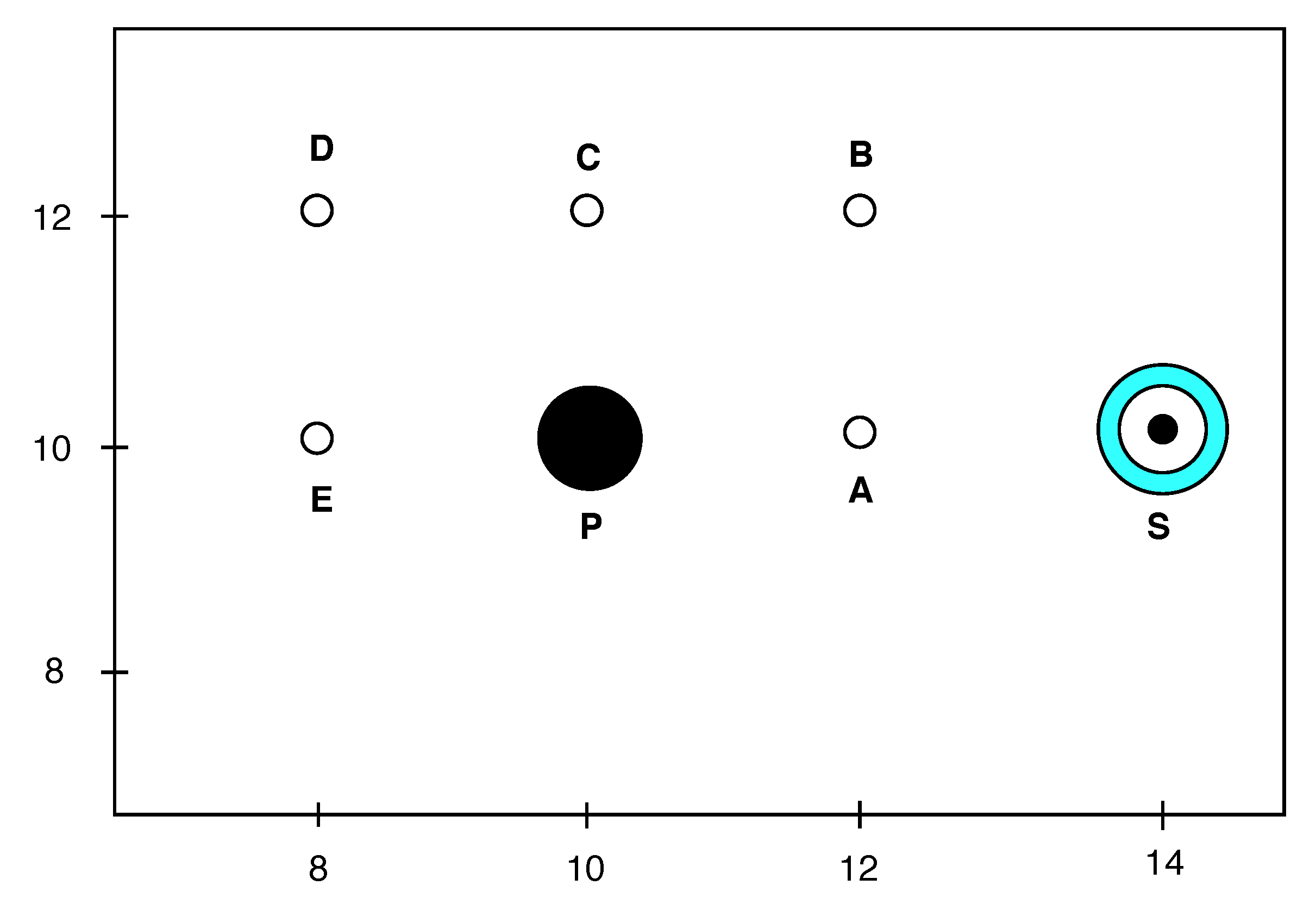The result was compared against the analytical solution of the linearized equations presented in [20]. In this case, the surface of the object was curved, and the wave did not only impinge in the normal direction of the obstacle. The expected symmetric scattering pattern of the reflected pulse eased the identification of numerical issues introduced by the modeling of the cylinder wall. Thus, this setting illustrated the treatment of curved boundaries in the high-order approximation scheme by penalization within simple square elements. The problem setup is depicted in Figure 10 and consisted of a cylinder of diameter $d=1.0$ with its center lying at the point P with the coordinates $(10,10)$.

The initial condition prescribed a circular Gaussian pulse in pressure with its center at the point $S=(14,10)$ and a half-width of $0.2$. Thus, the initial condition for the perturbation of pressure is given by:

$$p^{\prime }=ϵ\exp \left[-\ln \left(2\right)\frac{{(x-14)}^2+{(y-10)}^2}{0.04}\right].$$

(41)

The amplitude $ϵ={10}^{-3}$ of the pulse was chosen to be sufficiently small to nearly match the full compressible Navier–Stokes simulation with the linear reference solution.

The initial condition in terms of the conservative variables was given as:

$$\rho ={\rho }_0+p^{\prime },m_1=m_2=0,e=c_{p}T-\frac{p}{\rho }.$$

(42)

Here, ${\rho }_0$ is the background density chosen as ${\rho }_0=1.0$. $m_1,m_2$ are the momentum in the x and y direction, respectively, and e is the total energy. T and $c_p$ are the temperature and specific heat at constant pressure, respectively. The ratio of specific heats was chosen to be $\gamma =1.4$. The Reynolds number used was $Re=5\times {10}^5$, calculated using the diameter of the cylinder $d=1.0$ as the characteristic length. Figure 10 shows the test case setup magnified around the area of interest.

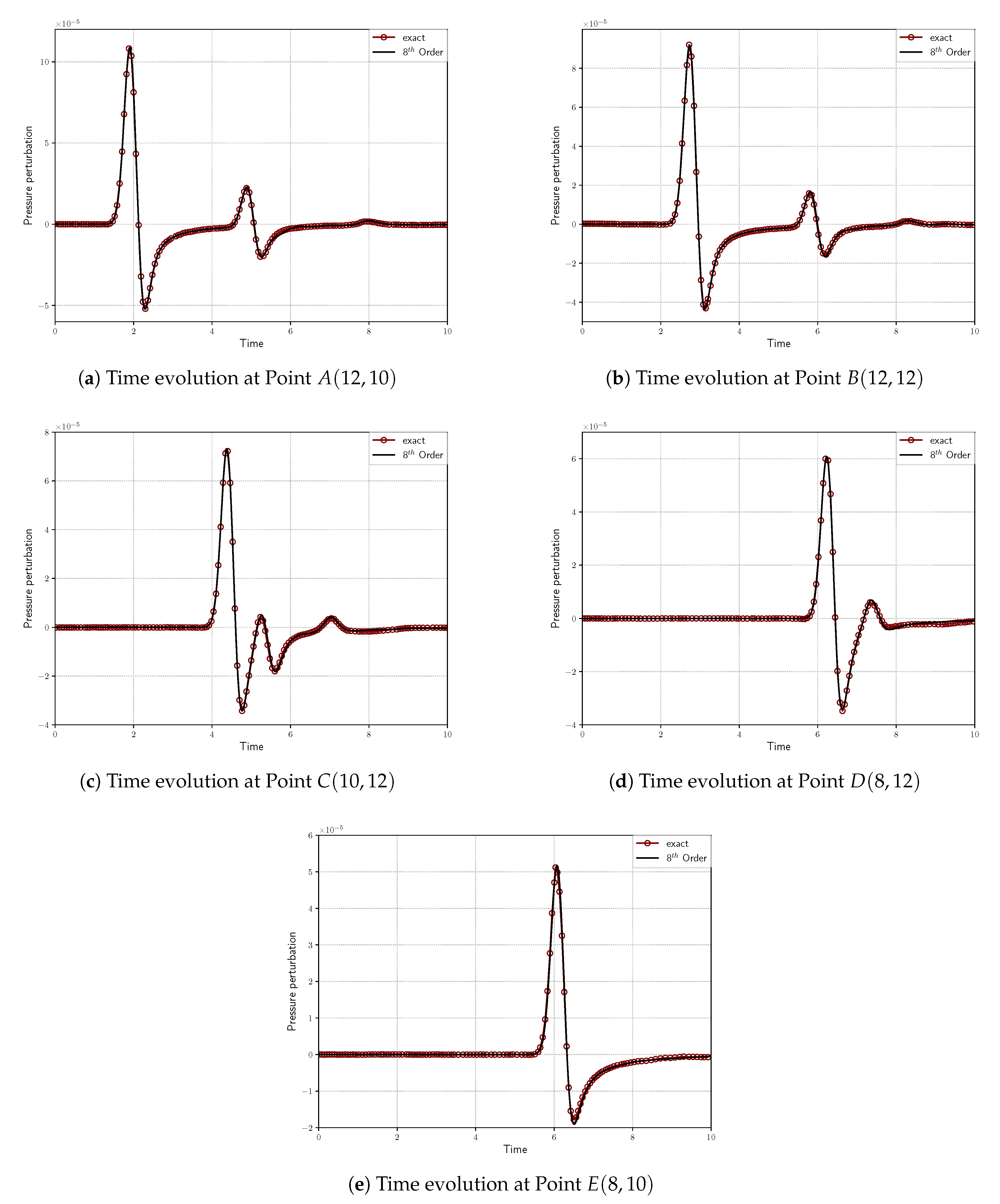
The overall simulation domain was $\Omega =[0,24]\times [0,20]$ to ensure that the boundaries were sufficiently far away to avoid interferences from reflections during the simulated time interval. To test the accuracy of the simulation, five probing points were chosen around the obstacle. The points were located in different directions with respect to the obstacle P and the source S. The incident and the reflected acoustic wave passed through these probes at different points in time. This intends to address both phase and amplitude errors that arise from the Brinkman penalization. The porosity was set to $\varphi =1.0$. The viscous and thermal permeability $\eta$ and ${\eta }_T$ were defined respectively with the help of the scaling parameter $\beta ={10}^{-6}$ according to Equations (33) and (34). Results were obtained solving the compressible Navier–Stokes equations in two dimensions with a spatial scheme order of $O=8$, i.e., 64 degrees of freedom per element. Cubical elements with an edge length of $dx=1/64$ were used to discretize the complete domain. The simulation was carried out for a total time of $t_{max}=10$ s.

The pressure perturbation in the initial condition resulted in the formation of an acoustic wave that propagated cylindrically outwards as depicted in Figure 11a. Eventually, the wave impinged on the obstacle, where it was reflected as shown in Figure 11b with the pressure perturbation at $t=4$. The quality of this reflected wave was completely dependent on the quality of the obstacle representation.

A third wave was generated when the initial wave, disrupted by the obstacle, traveled further to the left and joined again. This is visible in Figure 11c, and its further evolution is visible in Figure 11d, which shows the pressure perturbation at $t=8$. These three circular acoustic waves had different centers (shifted along the x-axis), but coincided left of the obstacle. As can be seen from these illustrations, the expected reflection pattern was nicely generated by the obstacle representation via the penalization. For a more quantitative assessment of the resulting simulation, we looked at the time evolution of the pressure perturbations at the chosen probing points.

Figure 12 shows the time evolution of the pressure fluctuations monitored at each of the five observation points around the cylinder. The numerical results were compared with the analytical solution for linear equations at these points. Here, we can observe the principal wave and the reflected wave arriving at different probing points at different times. We also observed that the computational results obtained showed an excellent agreement with the analytical solution for all the probes. It nearly perfectly predicted all the amplitudes and pressure behavior without showing phase shifts.

4. Conclusions

We showed that, with the help of an implicit mixed explicit time integration approach, it was feasible to implement wall boundaries accurately in a high-order discontinuous Galerkin scheme. The additional source terms introduced for the penalization can be efficiently computed in the implicit part of the mixed time integration without the need for iterative solvers. This implicit treatment enabled us to utilize arbitrary small values for the permeabilities and freed us from the need for the porosity introduced by Liu and Vasiliyev for compressible flows. The viability of the approach was shown in one-dimensional examples, where we saw that the solid wall can be well approximated with small permeabilities in the high-order discontinuous Galerkin scheme. Even for the reflection of a shock wave, for which a high-order discretization is problematic due to the oscillations incurred by the discontinuity, the penalization provided small errors and convergence with higher polynomial degrees. The real strength of the penalization method, however, came through in multiple dimensions, where curved boundaries could easily be represented by the penalization consistent with the scheme. As an example of such a setting, we looked at the acoustic wave scattering at a cylinder.

With the presented method, it, therefore, was possible to exploit the benefit of reduced memory consumption by the high-order discretization even for complex geometries without the need for advanced mesh generation.

References

1. Thompson, J.F.; Warsi, Z.U.; Mastin, C.W. Boundary-fitted coordinate systems for numerical solution of partial differential equations A review. J. Comput. Phys. 1982, 47, 1–108. [Google Scholar] [CrossRef]
2. Mittal, R.; Iaccarino, G. Immersed Boundary Methods. Annu. Rev. Fluid Mech. 2005, 37, 239–261. [Google Scholar] [CrossRef]
3. Peskin, C.S. Flow patterns around heart valves: A numerical method. J. Comput. Phys. 1972, 10, 252–271. [Google Scholar] [CrossRef]
4. Saiki, E.; Biringen, S. Numerical Simulation of a Cylinder in Uniform Flow: Application of a Virtual Boundary Method. J. Comput. Phys. 1996, 123, 450–465. [Google Scholar] [CrossRef]
5. Brown-Dymkoski, E.; Kasimov, N.; Vasilyev, O.V. A characteristic based volume penalization method for general evolution problems applied to compressible viscous flows. J. Comput. Phys. 2014, 262, 344–357. [Google Scholar] [CrossRef] [Green Version]
6. Arquis, E.; Caltagirone, J.P. Sur les conditions hydrodynamiques au voisinage d’une interface milieu fluide-milieu poreux: Application a’ la convection naturelle. CR Acad. Sci. Paris II 1984, 299, 1–4. [Google Scholar]
7. Angot, P.; Bruneau, C.H.; Fabrie, P. A penalization method to take into account obstacles in incompressible viscous flows. Numer. Math. 1999, 81, 497–520. [Google Scholar] [CrossRef]
8. Kevlahan, N.K.R.; Ghidaglia, J.M. Computation of turbulent flow past an array of cylinders using a spectral method with Brinkman penalization. Eur. J. Mech. B/Fluids 2001, 20, 333–350. [Google Scholar] [CrossRef] [Green Version]
9. Liu, Q.; Vasilyev, O.V. A Brinkman penalization method for compressible flows in complex geometries. J. Comput. Phys. 2007, 227, 946–966. [Google Scholar] [CrossRef]
10. Jause-Labert, C.; Godeferd, F.; Favier, B. Numerical validation of the volume penalization method in three-dimensional pseudo-spectral simulations. Comput. Fluids 2012, 67, 41–56. [Google Scholar] [CrossRef]
11. Pasquetti, R.; Bwemba, R.; Cousin, L. A pseudo-penalization method for high Reynolds number unsteady flows. Appl. Numer. Math. 2008, 58, 946–954. [Google Scholar] [CrossRef]
12. Ramière, I.; Angot, P.; Belliard, M. A fictitious domain approach with spread interface for elliptic problems with general boundary conditions. Comput. Methods Appl. Mech. Eng. 2007, 196, 766–781. [Google Scholar] [CrossRef] [Green Version]
13. Simulationstechnik und Wissenschaftliches Rechnen Uni Siegen. Ateles Source Code. 2019. Available online: https://osdn.net/projects/apes/scm/hg/ateles/ (accessed on 26 August 2019).
14. Alexander, R. Diagonally Implicit Runge–Kutta Methods for Stiff O.D.E.’s. SIAM J. Numer. Anal. 1977, 14, 1006–1021. [Google Scholar] [CrossRef]
15. Zudrop, J. Efficient Numerical Methods for Fluid- and Electrodynamics on Massively Parallel Systems. Ph.D. Thesis, RWTH Aachen University, Aachen, Germany, 2015. [Google Scholar]
16. Hesthaven, J.S.; Warburton, T. Nodal Discontinuous Galerkin Methods: Algorithms, Analysis, and Applications, 1st ed.; Springer: New York, NY, USA, 2007. [Google Scholar]
17. Piquet, A.; Roussel, O.; Hadjadj, A. A comparative study of Brinkman penalization and direct-forcing immersed boundary methods for compressible viscous flows. Comput. Fluids 2016, 136, 272–284. [Google Scholar] [CrossRef]
18. Ben-Dor, G.; Igra, O.; Elperin, T. (Eds.) Handbook of Shock Waves; Academic Press: Cambridge, MA, USA, 2001. [Google Scholar]
19. Glazer, E.; Sadot, O.; Hadjadj, A.; Chaudhuri, A. Velocity scaling of a shock wave reflected off a circular cylinder. Phys. Rev. E 2011, 83, 066317. [Google Scholar] [CrossRef]
20. Tam, C.K.W.; Hardin, J.C. Second Computational Aeroacoustics (CAA) Workshop on Benchmark Problems; NASA, Langley Research Center: Hampton, VA, USA, 1997.
Figure 1. One-dimensional acoustic wave setup: the center of the initial pressure pulse is located at x = 0.25 and has an amplitude of ϵ = 10 3 . Discretization by 48 elements as denoted by grid lines, and the right half of the domain ( x > 0.5 ) is penalized. Note that the wall coincides with an element interface.
Symmetry 11 01126 g001
Figure 2. Plot for the pressure profile of the reflected wave at t = 0.5 for different scaling factors β . The numerical reference is obtained with a traditional wall boundary condition and a high resolution.
Symmetry 11 01126 g002
Figure 3. Plot of the error in the wave amplitude at t = 0.5 with decreasing porosity and different scaling factors β . The error e is given by the relative error in the pulse amplitude after the reflection at the wall.
Symmetry 11 01126 g003
Figure 4. L 2 -error for a polynomial degree of seven over an increasing number of elements (h-refinement).
Symmetry 11 01126 g004
Figure 5. L 2 -error for 24 elements over increasing maximal polynomial degree (p-refinement).
Symmetry 11 01126 g005
Figure 6. L 2 -error for varying the polynomial degree. With a wall just 5% of the element length away from the element surface.
Symmetry 11 01126 g006
Figure 7. Behavior of the error in the reflected acoustic pulse with respect to computational effort. The figure on the left (a) shows the error convergence for various spatial orders over the required memory in terms of degrees of freedom. The right figure (b) shows the same runs, but now over the computational effort in terms of running time in seconds. All simulations were performed on a single node with 12 cores using 12 processes.
Symmetry 11 01126 g007
Figure 8. Different curves represent different discretizations using different scheme orders and a different number of elements. (a) Normalized pressure of the reflected shock wave. (b) Zoom of the reflected shock.
Symmetry 11 01126 g008
Figure 9. Different curves represent different locations of the porous material in the element and the solution when using a no-slip wall. (a) illustrates the normalized pressure of the reflected shock wave, and (b) depicts a zoom-in of the front area of the reflected shock.
Symmetry 11 01126 g009
Figure 10. Test case setup for the wave scattering; only the section containing the cylindrical obstacle, the probing points, and the initial pulse is shown, and the actual computational domain is larger. The cylindrical obstacle is represented by the black circle located at P ( 10 , 10 ) . Five observation points ( A , , E ) around the obstacle are shown as circles. The initial pulse in pressure is indicated by the black dot with a turquoise circle around it located at S ( 14 , 10 ) .
Symmetry 11 01126 g010
Figure 11. Simulation snapshots of pressure perturbations captured at successive points in time. The cylindrical obstacle is visible as a black disk and the probe points surrounding it as white dots. The scale of the pressure perturbation is kept constant for all snapshots.
Symmetry 11 01126 g011
Figure 12. Time evolution of pressure perturbations at all five observation points surrounding the cylinder up to t = 10 . Be aware that the perturbation pressure plotted along the y axis is scaled differently from probe to probe to illustrate the pressure profile better.
Symmetry 11 01126 g012