A Convex Combination Approach for Mean-Based Variants of Newton’s Method

Abstract

Several authors have designed variants of Newton’s method for solving nonlinear equations by using different means. This technique involves a symmetry in the corresponding fixed-point operator. In this paper, some known results about mean-based variants of Newton’s method (MBN) are re-analyzed from the point of view of convex combinations. A new test is developed to study the order of convergence of general MBN. Furthermore, a generalization of the Lehmer mean is proposed and discussed. Numerical tests are provided to support the theoretical results obtained and to compare the different methods employed. Some dynamical planes of the analyzed methods on several equations are presented, revealing the great difference between the MBN when it comes to determining the set of starting points that ensure convergence and observing their symmetry in the complex plane.

1. Introduction

We consider the problem of finding a simple zero $\alpha$ of a function $f:I\subset \mathbb{R}\to \mathbb{R}$, defined in an open interval I. This zero can be determined as a fixed point of some function g by means of the one-point iteration method:

$$x_{n+1}=g(x_n),n=0,1,\dots ,$$

(1)

where $x_0$ is the starting point. The most widely-used example of these kinds of methods is the classical Newton’s method given by:

$$x_{n+1}=x_n-\frac{f(x_n)}{f^{\prime }(x_n)},n=0,1,\dots .$$

(2)

It is well known that it converges quadratically to simple zeros and linearly to multiple zeros. In the literature, many modifications of Newton’s scheme have been published in order to improve its order of convergence and stability. Interesting overviews about this area of research can be found in [1,2,3]. The works of Weerakoon and Fernando [4] and, later, Özban [5] have inspired a whole set of variants of Newton’s method, whose main characteristic is the use of different means in the iterative expression.

It is known that if a sequence ${\{x_n\}}_{n\ge 0}$ tends to a limit $\alpha$ in such a way that there exist a constant $C>0$ and a positive integer $n_0$ such that:

$$|x_{n+1}-\alpha |\le C|x_n{-\alpha |}^p,\forall n\ge n_0,$$

(3)

for $p\ge 1$, then p is called the order of convergence of the sequence and C is known as the asymptotic error constant. For $p=1$, constant C satisfies $0<C\le 1$.

If we denote by $e_n=x_n-\alpha$ the exact error of the nth iterate, then the relation:

$$e_{n+1}=C{e}_n^p+\mathcal{O}(e_n^{p+1})$$

(4)

is called the error equation for the method and p is the order of convergence.

Let us suppose that $f:I\subseteq \mathbb{R}\to \mathbb{R}$ is a sufficiently-differentiable function and $\alpha$ is a simple zero of f. It is plain that:

$$f(x)=f(x_n)+{\int }_{x_n}^x{f}^{\prime }(t)dt.$$

(5)

Weerakoon and Fernando in [4] approximated the definite integral (5) by using the trapezoidal rule and taking $x=\alpha$, getting:

$$0\approx f(x_n)+1/2(\alpha -x_n)(f^{\prime }(x_n)+f^{\prime }(\alpha )),$$

(6)

and therefore, a new approximation $x_{n+1}$ to $\alpha$ is given by:

$$\begin{array}{ccc}\hfill x_{n+1}=x_n-\frac{f(x_n)}{(f^{\prime }(x_n)+f^{\prime }(z_n))/2},& \hfill & \hfill z_n=x_n-\frac{f(x_n)}{f^{\prime }(x_n)},n=0,1,\dots .\end{array}$$

(7)

Thus, this variant of Newton’s scheme can be considered to be obtained by replacing the denominator $f^{\prime }(x_n)$ of Newton’s method (2) by the arithmetic mean of $f^{\prime }(x_n)$ and $f^{\prime }(z_n)$. Therefore, it is known as the arithmetic mean Newton method (AN).

In a similar way, the arithmetic mean can be replaced by other means. In particular, the harmonic mean $M_{Ha}(x,y)=2xy/(x+y)$, where x and y are two nonnegative real numbers, from a different point of view:

$$M_{Ha}(x,y)=\frac{2xy}{x+y}=x\underset{\theta }{\underbrace{\frac{y}{x+y}}}+y\underset{1-\theta }{\underbrace{\frac{x}{x+y}}},$$

(8)

where since $0\le y\le x+y$, then $0\le \theta \le 1$, i.e., the harmonic mean can be seen as a convex combination between x and y, where every element is given the relevance of the other one in the sum. Now, let us switch the roles of x and y; we get:

$$x\frac{x}{x+y}+y\frac{y}{x+y}=\frac{x^2+y^2}{x+y}=M_{Ch}(x,y),$$

(9)

that is the contraharmonic mean between x and y.

Özban in [5] used the harmonic mean instead of the arithmetic one, which led to a new method:

$$x_{n+1}=x_n-\frac{f(x_n)(f^{\prime }(x_n)+f^{\prime }(z_n))}{2f^{\prime }(x_n)f^{\prime }(z_n)},n=0,1,\dots ,$$

(10)

being $z_n$ a Newton step, which he called the harmonic mean Newton method (HN).

Ababneh in [6] designed an iterative method associated with this mean, called the contraharmonic mean Newton method (CHN), whose iterative expression is:

$$x_{n+1}=x_n-\frac{(f^{\prime }(x_n)+f^{\prime }(z_n))f(x_n)}{f^{\prime }{(x_n)}^2+f^{\prime }{(z_n)}^2},$$

(11)

with third-order of convergence for simple roots of $f(x)=0$, as well as the methods proposed by Weerakoon and Fernando [4] and Özban [5].

This idea has been used by different authors for designing iterative methods applying other means, generating symmetric fixed point operators. For example, Xiaojian in [7] employed the generalized mean of order $m\in \mathbb{R}$ between two values x and y defined as:

$$M_G(x,y)={\left(\frac{x^m+y^m}{2}\right)}^{1/m},$$

(12)

to construct a third-order iterative method for solving nonlinear equations. Furthermore Singh et al. in [8] presented a third-order iterative scheme by using the Heronian mean between two values x and y, defined as:

$$M_{He}(x,y)=\frac{1}{3}(x+\sqrt{xy}+y).$$

(13)

Finally, Verma in [9], following the same procedure, designed a third-order iterative method by using the centroidal mean between two values x and y, defined as:

$$M_{Ce}(x,y)=\frac{2(x^2+xy+y^2)}{3(x+y)}.$$

(14)

In this paper, we check that all these means are functional convex combinations means and develop a simple test to prove easily the third-order of the corresponding iterative methods, mentioned before. Moreover, we introduce a new method based on the Lehmer mean of order $m\in \mathbb{R}$, defined as:

$$M_{L_m}(x,y)=\frac{x^m+y^m}{x^{m-1}+y^{m-1}}$$

(15)

and propose a generalization that also satisfies the previous test. Finally, all these schemes are numerically tested, and their dependence on initial estimations is studied by means of their basins of attraction. These basins are shown to be clearly symmetric.

The rest of the paper is organized as follows: Section 2 is devoted to designing a test that allows us to characterize the third-order convergence of the iterative method defined by a mean. This characterization is used in Section 3 for giving an alternative proof of the convergence of mean-based variants of Newton’s (MBN) methods, including some new ones. In Section 4, we generalize the previous methods by using the concept of $\sigma$-means. Section 5 is devoted to numerical results and the use of basins of attraction in order to analyze the dependence of the iterative methods on the initial estimations used. With some conclusions, the manuscript is finished.

2. Convex Combination

In a similar way as has been stated in the Introduction for the arithmetic, harmonic, and contraharmonic means, the rest of the mentioned means can be also regarded as convex combinations. This is not coincidental: one of the most interesting properties that a mean satisfies is the averaging property:

$$min(x,y)\le M(x,y)\le max(x,y),$$

(16)

where $M(x,y)$ is any mean function of x and y nonnegative. This implies that every mean that satisfies this property is a certain convex combination among its terms.

Indeed, there exists a unique $\theta (x,y))\in [0,1]$ such that:

$$\theta (x,y)=\left\{\begin{array}{cc}\frac{M(x,y)-y}{x-y}\hfill & \mathrm{if}x\ne y\hfill \\ 0\hfill & \mathrm{if}x=y\hfill \end{array}\right..$$

(17)

This approach suggests that it is possible to generalize every mean-based variant of Newton’s method (MBN), by studying their convex combination counterparts. As a matter of fact, every mean-based variant of Newton’s method can be rewritten as:

$$x_{n+1}=x_n-\frac{f(x_n)}{\theta f^{\prime }(x_n)+(1-\theta )f^{\prime }(z_n)},$$

(18)

where $\theta =\theta (f^{\prime }(x_n),f^{\prime }(z_n))$. This is a particular case of a family of iterative schemes constructed in [10].

We are interested in studying its order of convergence as a function of $\theta$. Thus, we need to compute the approximated Taylor expansion of the convex combination at the denominator and then its inverse:

$$\begin{array}{cc}\hfill \theta f^{\prime }(x_n)+(1-\theta )f^{\prime }(z_n)& =\theta f^{\prime }(\alpha )[1+2c_2{e}_n+3c_3{e}_n^2+4c_4{e}_n^3+\mathcal{O}(e_n^4)]+\hfill \\ \hfill & \phantom{=}+(1-\theta )f^{\prime }(\alpha )[1+2c_2{e}_n^2+4c_2(c_3-c_2^2)e_n^3+\mathcal{O}(e_n^4)]\hfill \\ \hfill & =f^{\prime }(\alpha )[\theta +2\theta c_2{e}_n+3\theta c_3{e}_n^2+4\theta c_4{e}_n^3+\mathcal{O}(e_n^4)]+\hfill \\ \hfill & \phantom{=}+f^{\prime }(\alpha )[1+2c_2^2{e}_n^2+4c_2(c_3-c_2^2)e_n^3+\mathcal{O}(e_n^4)]+\hfill \\ \hfill & \phantom{=}-f^{\prime }(\alpha )[\theta +2\theta c_2^2{e}_n^2+4\theta c_2(c_3-c_2^2)e_n^3+\mathcal{O}(e_n^4)]\hfill \\ \hfill & =f^{\prime }(\alpha )[1+2\theta c_2{e}_n+(2c_2^2+3\theta c_3-2\theta c_2^2+3\theta c_3)e_n^2]+\hfill \\ \hfill & \phantom{=}+f^{\prime }(\alpha )[(4\theta c_4+(1-\theta )4c_2(c_3-c_2^2))e_n^3+\mathcal{O}(e_n^4)];\hfill \end{array}$$

(19)

where $c_j={\displaystyle \frac{1}{j!}}{\displaystyle \frac{f^{(j)}(\alpha )}{f^{\prime }(\alpha )}},j=1,2,\dots$. Then, its inverse can be expressed as:

$$\begin{array}{cc}\hfill & f^{\prime }{(\alpha )}^{-1}(1-[2\theta c_2{e}_n+(2c_2^2+3\theta c_3-2\theta c_2^2+3\theta c_3)e_n^2+(4\theta c_4+(1-\theta )4c_2(c_3-c_2^2))e_n^3+\mathcal{O}(e_n^4)]+\hfill \\ \hfill & \phantom{f^{\prime }{(\alpha )}^{-1}}+{[2\theta c_2{e}_n+(2c_2^2+3\theta c_3-2\theta c_2^2+3\theta c_3)e_n^2+(4\theta c_4+(1-\theta )4c_2(c_3-c_2^2))e_n^3+\mathcal{O}(e_n^4)]}^2-\cdots )\hfill \\ \hfill =& f^{\prime }{(\alpha )}^{-1}[1-2\theta c_2{e}_n+(2\theta c_2^2-2c_2^2+4{\theta }^2{c}_2^2-3\theta c_3)e_n^2-(4\theta c_4+(1-\theta )4c_2(c_3-c_2^2))e_n^3+\mathcal{O}(e_n^4)].\hfill \end{array}$$

(20)

Now,

$$\frac{f(x_n)}{\theta f^{\prime }(x_n)+(1-\theta )f^{\prime }(z_n)}=e_n+c_2(1-2\theta )e_n^2+(4{\theta }^2{c}_2^2-2c_2^2+c_3-3\theta c_3)e_n^3+\mathcal{O}(e_n^4),$$

(21)

and by replacing it in (18), it leads to the MBN error equation as a function of $\theta$:

$$e_{n+1}=-c_2(1-2\theta )e_n^2-(4{\theta }^2{c}_2^2-2c_2^2+c_3-3\theta c_3)e_n^3+\mathcal{O}(e_n^4)≕\Phi (\theta ).$$

(22)

Equation (22) can be used to re-discover the results of convergence: for example, for the contraharmonic mean, we have:

$$\theta (f^{\prime }(x_n),f^{\prime }(z_n))=\frac{f^{\prime }(x_n)}{f^{\prime }(x_n)+f^{\prime }(z_n)},$$

(23)

where:

$$f^{\prime }(x_n)+f^{\prime }(z_n)=2f^{\prime }(\alpha )[1+c_2{e}_n(c_2^2-3/2c_3)e_n^2+2(c_2{c}_3-c_2^3+c_4)e_n^3+\mathcal{O}(e_n^4)],$$

(24)

so that:

$$\begin{array}{cc}\hfill \frac{1}{f^{\prime }(x_n)+f^{\prime }(z_n)}& ={(2f^{\prime }(\alpha ))}^{-1}[1-c_2{e}_n-3/2c_3{e}_n^2+4c_2^3{e}_n^3-2c_4{e}_n^3+c_2{c}_3{e}_n^3+\mathcal{O}(e_n^4)]\hfill \\ \hfill & ={(2f^{\prime }(\alpha ))}^{-1}[1-c_2{e}_n-3/2c_3{e}_n^2+(4c_2^3-2c_4+c_2{c}_3)e_n^3+\mathcal{O}(e_n^4)].\hfill \end{array}$$

(25)

Thus, we can obtain the $\theta$ associated with the contraharmonic mean:

$$\begin{array}{cc}\hfill \theta (f^{\prime }(x_n),f^{\prime }(z_n))& =[1/2+c_2{e}_n+3/2c_3{e}_n^2+2c_4{e}_n^3+\mathcal{O}(e_n^4)]·\hfill \\ \hfill & \phantom{=}·[1-c_2{e}_n-3/2c_3{e}_n^2+(4c_2^3+c_2{c}_3-2c_4)e_n^3+\mathcal{O}(e_n^4)]\hfill \\ \hfill & =1/2+1/2c_2{e}_n-c_2^2{e}_n^2+3/4c_3{e}_n^2+2c_2^3{e}_n^3+c_4{e}_n^3-5/2c_2{c}_3{e}_n^3+\mathcal{O}(e_n^4)\hfill \\ \hfill & =1/2+1/2c_2{e}_n+(3/4c_3-c_2^2)e_n^2+(2c_2^3+c_4-5/2c_2{c}_3)e_n^3+\mathcal{O}(e_n^4).\hfill \end{array}$$

(26)

Finally, by replacing the previous expression in (22):

$$e_{n+1}=(1/2c_3+2c_2^2)e_n^3+\mathcal{O}(e_n^4),$$

(27)

and we obtain again that the convergence for the contraharmonic mean Newton method is cubic.

Regarding the harmonic mean, it is straightforward that it is a functional convex combination, with:

$$\begin{array}{cc}\hfill \theta (f^{\prime }(x_n),f^{\prime }(z_n))& =1-\frac{f^{\prime }(x_n)}{f^{\prime }(x_n)+f^{\prime }(z_n)}\hfill \\ \hfill & =1/2+1/2c_2{e}_n+(c_2^2-3/4c_3)e_n^2+(5/2c_2{c}_3-2c_2^3-c_4)e_n^3+\mathcal{O}(e_n^4).\hfill \end{array}$$

(28)

Replacing this expression in (22), we find the cubic convergence of the harmonic mean Newton method,

$$e_{n+1}=1/2c_3{e}_n^3+\mathcal{O}(e_n^4).$$

(29)

In both cases, the independent term of $\theta (f^{\prime }(x_n),f^{\prime }(z_n))$ was $1/2$; it was not a coincidence, but an instance of the following more general result.

Theorem 1.

Let $\theta =\theta (f^{\prime }(x_n),f^{\prime }(z_n))$ be associated with the mean-based variant of Newton’s method (MBN):

$$\begin{array}{ccc}\hfill x_{n+1}=x_n-\frac{f(x_n)}{M(f^{\prime }(x_n),f^{\prime }(z_n))},& \hfill & \hfill z_n=x_n-\frac{f(x_n)}{f^{\prime }(x_n)},\end{array}$$

(30)

where M is a mean function of the variables $f^{\prime }(x_n)$ and $f^{\prime }(z_n)$. Then, MBN converges, at least, cubically if and only if the estimate:

$$\theta =1/2+\mathcal{O}(e_n).$$

(31)

holds.

Proof. 

We replace $\theta =1/2+\mathcal{O}(e_n)$ in the MBN error Equation (22), obtaining:

$$e_{n+1}=(4{\theta }^2{c}_2^2-2c_2^2+c_3-3\theta c_3)e_n^3+\mathcal{O}(e_n^4).\hspace{1em}☐$$

(32)

Now, some considerations follow.

Remark 1.

Generally speaking,

$$\theta =a_0+a_1{e}_n+a_2{e}_n^2+a_3{e}_n^3+\mathcal{O}(e_n^4),$$

(33)

where $a_i$ are real numbers. If we put (33) in (22), we have:

$$e_{n+1}=-c_2(1-2a_0)e_n^2-(4a_0^2{c}_2^2-3a_0{c}_3-2a_1{c}_2-2c_2^2+c_3)e_n^3+\mathcal{O}(e_n^4);$$

(34)

it follows that, in order to attain cubic convergence, the coefficient of $e_n^2$ must bezero. Therefore, $a_0(u)=1/2$. On the other hand, to achieve a higher order (i.e., at least four), we need to solve the following system:

$$\left\{\begin{array}{ccc}1-2a_0& =& 0\\ 4a_0^2{c}_2^2-3a_0{c}_3-2a_1{c}_2-2c_2^2+c_3& =& 0\end{array}\right..$$

(35)

This gives us that $a_0(u)=1/2,a_1(u)=-1/4(2c_2^2+c_3)/(c_2)$ assure at least a fourth-order convergence of the method. However, none of the MBN methods under analysis satisfy these conditions simultaneously.

Remark 2.

The only convex combination involving a constant θ that converges cubically is $\theta =1/2$, i.e., the arithmetic mean.

The most useful aspect of Theorem 1 is synthesized in the following corollary, which we call the “$\theta$-test”.

Corollary 1 (θ-test)

With the same hypothesis of Theorem 1, an MBN converges at least cubically if and only if the Taylor expansion of the mean holds:

$$M(f^{\prime }(x_n),f^{\prime }(z_n))=f^{\prime }(\alpha )\left[1+\frac{1}{2}{c}_2{e}_n\right]+\mathcal{O}(e_n^2).$$

(36)

Let us notice that Corollary 1 provides a test to analyze the convergence of an MBN without having to find out the inherent $\theta$, therefore sensibly reducing the overall complexity of the analysis.

Re-Proving Known Results for MBN

In this section, we apply Corollary 1 to prove the cubic convergence of known MBN via a convex combination approach.

(i)

Arithmetic mean:

$$\begin{array}{cc}\hfill M_A(f^{\prime }(x_n),f^{\prime }(z_n))& =\frac{f^{\prime }(x_n)+f^{\prime }(z_n)}{2}\hfill \\ \hfill & =\frac{1}{2}\left(f^{\prime }(\alpha )[1+2c_2{e}_n+\mathcal{O}(e_n^2)]+f^{\prime }(\alpha )[1+\mathcal{O}(e_n^2)]\right)\hfill \\ \hfill & =f^{\prime }(\alpha )[1+c_2{e}_n+\mathcal{O}(e_n^2)].\hfill \end{array}$$

(37)

(ii)

Heronian mean: In this case, the associated $\theta$-test is:

$$\begin{array}{cc}\hfill M_{He}{f}^{\prime }(x_n),f^{\prime }(z_n)& =\frac{1}{3}\left(f^{\prime }(\alpha )[1+2c_2{e}_n+\mathcal{O}(e_n^2)]+f^{\prime }(\alpha )[1+c_2{e}_n+\mathcal{O}(e_n^2)]+f^{\prime }(\alpha )[1+\mathcal{O}(e_n^2)]\right)\hfill \\ \hfill & =\frac{f^{\prime }(\alpha )}{3}[3+2c_2{e}_n+c_2{e}_n+\mathcal{O}(e_n^2)].\hfill \end{array}$$

(38)

(iii)

Generalized mean:

$$\begin{array}{cc}\hfill M_G(f^{\prime }(x_n),f^{\prime }(z_n))& ={\left(\frac{f^{\prime }{(x_n)}^m+f^{\prime }{(z_n)}^m)}{2}\right)}^{1/m}\hfill \\ \hfill & ={\left(\frac{f^{\prime }{(\alpha )}^m{[1+2c_2{e}_n+\mathcal{O}(e_n^2)]}^m+f^{\prime }{(\alpha )}^m{[1+\mathcal{O}(e_n^2)]}^m}{2}\right)}^{1/m}\hfill \\ \hfill & =f^{\prime }(\alpha ){\left({[1+c_2{e}_n+\mathcal{O}(e_n^2)]}^m\right)}^{1/m}\hfill \\ \hfill & =f^{\prime }(\alpha )[1+c_2{e}_n+\mathcal{O}(e_n^2)].\hfill \end{array}$$

(39)

(iv)

Centroidal mean:

$$\begin{array}{cc}\hfill M_{Ce}(f^{\prime }(x_n),f^{\prime }(z_n))& =\frac{2(f^{\prime }{(x_n)}^2+f^{\prime }(x_n)f^{\prime }(z_n)+f^{\prime }(z_n))}{3(f^{\prime }(x_n)+f^{\prime }(z_n))}\hfill \\ \hfill & =\frac{2(f^{\prime }{(\alpha )}^2[1+2c_2{e}_n+\mathcal{O}(e_n^2)]+f^{\prime }{(\alpha )}^2[2+4c_2{e}_n+\mathcal{O}(e_n^2)])}{3(f^{\prime }(\alpha )[2+2c_2{e}_n+\mathcal{O}(e_n^2)])}\hfill \\ \hfill & =\frac{2(f^{\prime }{(\alpha )}^2[3+6c_2{e}_n+\mathcal{O}(e_n^2)])}{3(f^{\prime }(\alpha )[2+2c_2{e}_n+\mathcal{O}(e_n^2)])}\hfill \\ \hfill & =f^{\prime }(\alpha )[1+2c_2{e}_n+\mathcal{O}(e_n^2)][1+c_2{e}_n+\mathcal{O}(e_n^2)]\hfill \\ \hfill & =f^{\prime }(\alpha )[1+c_2{e}_n+\mathcal{O}(e_n^2)].\hfill \end{array}$$

(40)

3. New MBN by Using the Lehmer Mean and Its Generalization

The iterative expression of the scheme based on the Lehmer mean of order $m\in \mathbb{R}$ is:

$$x_{n+1}=x_n-\frac{f(x_n)}{M_{L_m}(f^{\prime }(x_n),f^{\prime }(z_n))},$$

where $z_n=x_n-\frac{f(x_n)}{f^{\prime }(x_n)}$ and:

$$M_{L_m}(f^{\prime }(x_n),f^{\prime }(z_n))=\frac{f^{\prime }{(x_n)}^m+f^{\prime }{(z_n)}^m}{f^{\prime }{(x_n)}^{m-1}+f^{\prime }{(z_n)}^{m-1}}.$$

(41)

Indeed, there are suitable values of parameter p such that the associated Lehmer mean equals the arithmetic one and the geometric one, but also the harmonic and the contraharmonic ones. In what follows, we will find it again, this time in a more general context.

By analyzing the associated $\theta$-test, we conclude that the iterative scheme designed with this mean has order of convergence three.

$$\begin{array}{cc}\hfill M_{L_m}(f^{\prime }(x_n),f^{\prime }(z_n))& =\frac{f^{\prime }{(x_n)}^m+f^{\prime }{(z_n)}^m}{f^{\prime }{(x_n)}^{m-1}+f^{\prime }{(z_n)}^{m-1}}\hfill \\ \hfill & =\frac{f^{\prime }{(\alpha )}^m{[1+2c_2{e}_n+\mathcal{O}(e_n^2)]}^m+f^{\prime }{(\alpha )}^m{[1+\mathcal{O}(e_n^2)]}^m}{f^{\prime }{(\alpha )}^{m-1}{[1+2c_2{e}_n+\mathcal{O}(e_n^2)]}^{m-1}+f^{\prime }{(\alpha )}^{m-1}{[1+\mathcal{O}(e_n^2)]}^{m-1}}\hfill \\ \hfill & =f^{\prime }(\alpha )[1+m{c}_2{e}_n+\mathcal{O}(e_n^2)]·[1-\left((m-1)c_2{e}_n+\mathcal{O}(e_n^2)\right)+{\left((m-1)c_2{e}_n+\mathcal{O}(e_n^2)\right)}^2+\dots ]\hfill \\ \hfill & =f^{\prime }(\alpha )[1+m{c}_2{e}_n+\mathcal{O}(e_n^2)]·[1-(m-1)c_2{e}_n+\mathcal{O}(e_n^2)]\hfill \\ \hfill & =f^{\prime }(\alpha )[1+c_2{e}_n+\mathcal{O}(e_n^2)].\hfill \end{array}$$

(42)

$\sigma$-Means

Now, we propose a new family of means of n variables, starting again from convex combinations. The core idea in this work is that, in the end, two distinct means only differ in their corresponding weights $\theta$ and $1-\theta$. In particular, we can regard the harmonic mean as an “opposite-weighted”mean, while the contraharmonic one is a “self-weighted”mean.

This behavior can be generalized to n variables:

$$M_{CH}(x_1,\dots ,x_n)=\frac{{\sum }_{i=1}^n{x}_i^2}{{\sum }_{i=1}^n{x}_i}$$

(43)

is the contraharmonic mean among n numbers. Equation (43) is just a particular case of what we call $\sigma$-mean.

Definition 1 (σ-mean)

Given $\mathbf{x}=(x_1,\dots ,x_n)\in {\mathbb{R}}^n$ a vector of n real numbers and a bijective map $\sigma :\{1,\dots ,n\}\to \{1,\dots ,n\}$ (i.e., $\sigma (\mathbf{x})$ is a permutation of $x_1,\dots ,x_n$), we call the σ-mean of order $m\in \mathbb{R}$ the real number given by:

$$M_{\sigma }(x_1,\dots ,x_n)\frac{{\displaystyle \sum _{i=1}^n{x}_i·x_{\sigma (i)}^m}}{{\displaystyle \sum _{j=1}^n{x}_j^m}}.$$

(44)

Indeed, it is easy to see that, in an $\sigma$-mean, the weight assigned to each node $x_i$ is:

$$\frac{x_{\sigma (i)}^m}{{\displaystyle \sum _{j=1}^n{x}_{\sigma (j)}^m}}=\frac{x_{\sigma (i)}^m}{{\displaystyle \sum _{j=1}^n{x}_j^m}}\in [0,1],$$

(45)

where the equality holds because $\sigma$ is a permutation of the indices. We are, therefore, still dealing with a convex combination, which implies that Definition 1 is well posed.

We remark that if we take $\sigma =\mathrm{𝟙}$, i.e., the identical permutation, in (44), we find the Lehmer mean of order m. Actually, the Lehmer mean is a very special case of the $\sigma$-mean, as the following result proves.

Proposition 1.

Given $m\in \mathbb{R}$, the Lehmer mean of order m is the maximum σ-mean of order m.

Proof. 

We recall the rearrangement inequality:

$$x_n{y}_1+\cdots +x_1{y}_n\le x_{\sigma (1)}{y}_1+\cdots +x_{\sigma (n)}{y}_n\le x_1{y}_1+\cdots +x_n{y}_n,$$

(46)

which holds for every choice of $x_1,\dots ,x_n$ and $y_1,\dots ,y_n$ regardless of the signs, assuming that both $x_i$ and $y_j$ are sorted in increasing order. In particular, $x_1<x_2<\cdots <x_n$ and $y_1<y_2<\cdots <y_n$ imply that the upper bound is attained only for the identical permutation.

Then, to prove the result, it is enough to replace every $y_i$ with the corresponding weight defined in (45). ☐

The Lehmer mean and $\sigma$-mean are deeply related: if $n=2$, as is the case of MBN, there are only two possible permutations, the identical one and the one that swaps one and two. We have already observed that the identical permutation leads to the Lehmer mean; however, if we express $\sigma$ in standard cycle notation as $\overline{\sigma }=(1,2)$, we have that:

$$M_{\overline{\sigma }}(x_1,x_2)=\frac{x_1{x}_2(x_1^m+x_2^m)}{x_1^{m+1}+x_2^{m+1}}=\frac{x_1^{-m}+x_2^{-m}}{x_1^{-m-1}+x_2^{-m-1}}=M_{L_{-m}}(x_1,x_2).$$

(47)

We conclude this section proving another property of $\sigma$-means, which is that the arithmetic mean of all possible $\sigma$-means of n numbers equals the arithmetic mean of the numbers themselves.

Proposition 2.

Given n real numbers $x_1,\dots ,x_n$ and ${\Sigma }_n$ denoting the set of all possible permutations of $\{1\dots ,n\}$, we have:

$$\frac{1}{n!}\sum _{\sigma \in {\Sigma }_n}{M}_{\sigma }(x_1,\dots ,x_n)=\frac{1}{n}\sum _{i=1}^n{x}_i$$

(48)

for all $m\in \mathbb{R}$.

Proof. 

Let us rewrite Equation (48); by definition, we have:

$$\frac{1}{n!}\sum _{\sigma \in {\Sigma }_n}{M}_{\sigma }(x_1,\dots ,x_n)=\frac{1}{n!}\sum _{\sigma \in {\Sigma }_n}\left(\frac{{\sum }_{i=1}^n{x}_i{x}_{\sigma (i)}^m}{{\sum }_{j=1}^n{x}_j^m}\right)=\frac{1}{n}\sum _{i=1}^n{x}_i$$

(49)

and we claim that the last equality holds. Indeed, we notice that every term in the sum of the $\sigma$-means on the left side of the last equality involves a constant denominator, so we can multiply both sides by it and also by $n!$ to get:

$$\sum _{\sigma \in {\Sigma }_n}\left(\sum _{i=1}^n{x}_i{x}_{\sigma (i)}^m\right)=(n-1)!\left(\sum _{j=1}^n{x}_j^m\right)\left(\sum _{i=1}^n{x}_i\right).$$

(50)

Now, it is just a matter of distributing the product on the right in a careful way:

$$(n-1)!\left(\sum _{j=1}^n{x}_j^m\right)\left(\sum _{i=1}^n{x}_i\right)=\sum _{i=1}^n\left(x_i·\sum _{k=1}^n\left((n-1)!\right)x_k^m\right),$$

(51)

If we fix $i\in \{1,\dots ,n\}$, in ${\Sigma }_n$, there are exactly $(n-1)!$ permutations $\sigma$ such that $\sigma (i)=i$. Therefore, the equality in (50) follows straightforwardly.

4. Numerical Results and Dependence on Initial Estimations

Now, we present the results of some numerical computations, in which the following test functions have been used.

(a)

$f_1(x)=x^3+4x^2-10$,

(b)

$f_2(x)=sin{(x)}^2-x^2+1$,

(c)

$f_3(x)=x^2-{\mathrm{e}}^x-3x+2$,

(d)

$f_4(x)=cos(x)-x$,

(e)

$f_5(x)={(x-1)}^3-1$.

The numerical tests were carried out by using MATLAB with double precision arithmetics in a computer with processor i7-8750H @2.20 GHz, 16 Gb of RAM, and the stopping criterion used was $|x_{n+1}-x_n|+|f(x_{n+1})|<{10}^{-14}$.

We used the harmonic mean Newton method (HN), the contraharmonic mean Newton method (CHN), the Lehmer mean Newton method (LN(m)), a variant of Newton’s method where the mean is a convex combination with $\theta =1/3$, $1/3$N, and the classic Newton method (CN). The main goals of these calculations are to confirm the theoretical results stated in the preceding sections and to compare the different methods, with CN as a control benchmark. In

Table 1. Numerical results. HN, the harmonic mean Newton method; CHN, the contraharmonic mean Newton method; LN, the Lehmer–Newton method; CN, the classic Newton method.

Function	x${}_0$	Number of Iterations					ACOC
		HN	CHN	LN(−7)	1/3 N	CN	HN	CHN	LN(−7)	1/3 N	CN
(a)	−0.5	50	18	55	6	132	3.10	3.03	2.97	1.99	2.00
	1	4	5	5	5	6	2.94	3.01	2.96	2.02	2.00
	2	4	5	5	5	6	3.10	2.99	3.02	2.00	2.00
(b)	1	4	5	6	6	7	3.06	3.16	3.01	2.01	2.00
	3	4	5	7	6	7	3.01	2.95	3.02	2.01	2.00
(c)	2	5	5	5	5	6	3.01	2.99	3.11	2.01	2.00
	3	5	6	5	6	7	3.10	3.00	3.10	2.01	2.00
(d)	−0.3	5	5	5	6	6	2.99	3.14	3.02	2.01	1.99
	1	4	4	4	5	5	2.99	2.87	2.88	2.01	2.00
	1.7	4	4	5	5	5	3.00	2.72	3.02	2.01	1.99
(e)	0	6	$>1000$	7	7	10	3.06	3.00	3.02	2.01	2.00
	1.5	5	7	7	7	8	3.04	3.01	2.99	2.01	2.00
	2.5	4	5	5	5	7	3.07	2.96	3.01	1.99	2.00
	3.0	5	6	6	6	7	3.04	2.99	2.98	2.00	2.00
	3.5	5	6	6	6	8	3.07	2.95	2.99	2.00	2.00

, we show the number of iterations that each method needs for satisfying the stopping criterion and also the approximated computational order of convergence, defined in [11], with the expression:

$$ACOC=\frac{ln(|x_{n+1}-x_n|/|x_n-x_{n-1}|)}{ln(|x_n-x_{n-1}|/|x_{n-1}-x_{n-2}|)},n=2,3,\dots ,$$

which is considered as a numerical approximation of the theoretical order of convergence p.

Regarding the efficiency of the MBN, we used the efficiency index defined by Ostrowski in [12] as $EI=p^{\frac{1}{d}}$, where p is the order of convergence of the method and d is the number of functional evaluations per iteration. In this sense, all the MBN had the same $E{I}_{MBN}=3^{\frac{1}{3}}$; meanwhile, Newton’s scheme had the index $E{I}_{CN}=2^{\frac{1}{2}}$. Therefore, all MBN were more efficient than the classical Newton method.

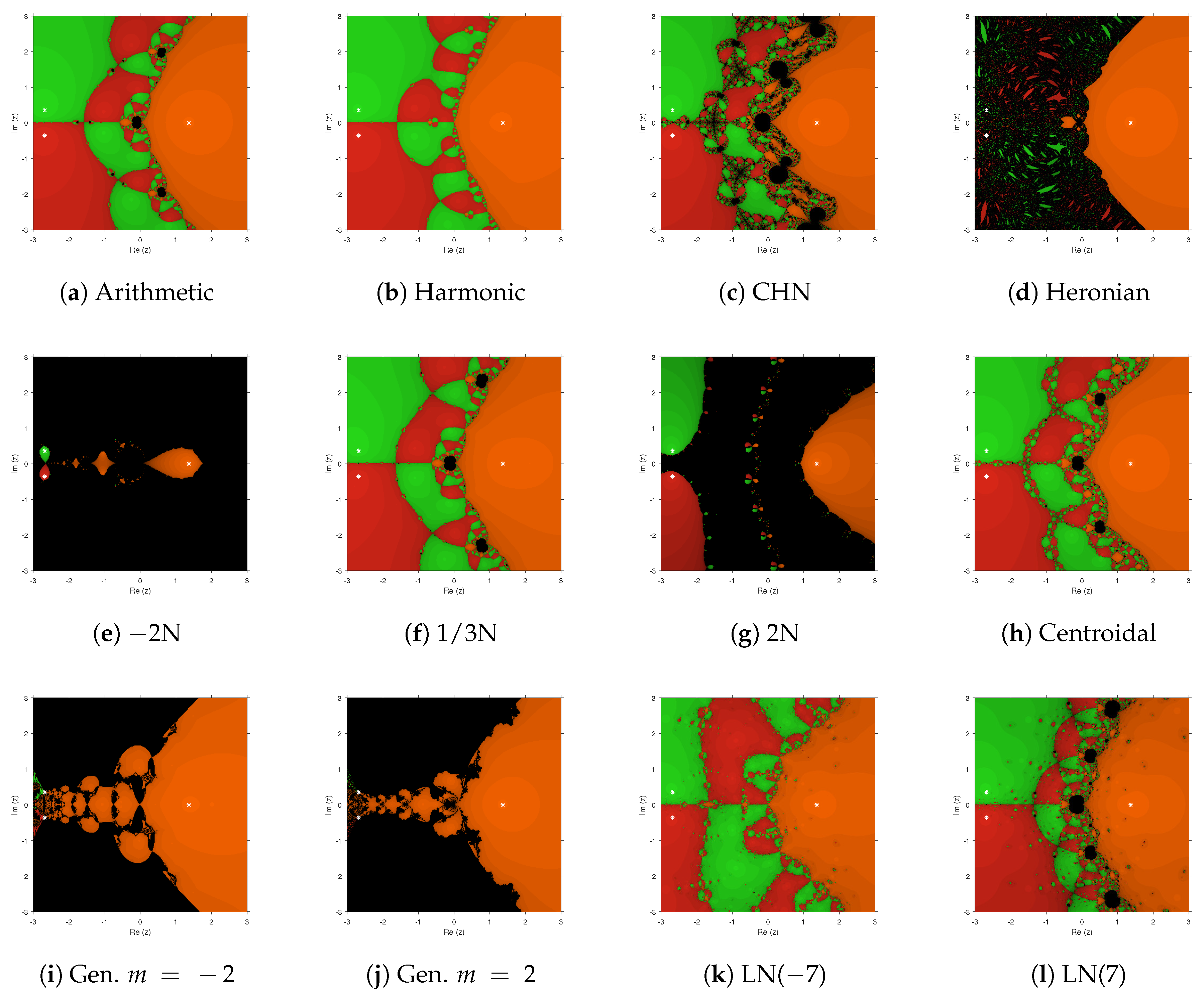
The presented numerical tests showed the performance of the different iterative methods to solve specific problems with fixed initial estimations and a stringent stopping criterion. However, it is useful to know their dependence on the initial estimation used. Although the convergence of the methods has been proven for real functions, it is usual to analyze the sets of convergent initial guesses in the complex plane (the proof would be analogous by changing the condition on the function to be differentiable by being holomorphic). To get this aim, we plotted the dynamical planes of each one of the iterative methods on the nonlinear functions $f_i(x)$, $i=1,2,\dots ,5$, used in the numerical tests. In them, a mesh of $400\times 400$ initial estimations was employed in the region of the complex plane $[-3,3]\times [-3,3]$.

We used the routines appearing in [13] to plot the dynamical planes corresponding to each method. In them, each point of the mesh was an initial estimation for the analyzed method on the specific problem. If the method reached the root in less than 40 iterations (closer than ${10}^{-3}$), then this point is painted in orange (green for the second, etc.) color; if the process converges to another attractor different from the roots, then the point is painted in black. The zeros of the nonlinear functions are presented in the different pictures by white stars.

In Figure 1, we observe that Harmonic and Lehmer (for $m=-7$) means showed the most stable performance, whose unique basins of attraction were those of the roots (plotted in orange, red, and green). In the rest of the cases, there existed black areas of no convergence to the zeros of the nonlinear function $f_1(x)$. Specially unstable were the cases of Heronian, convex combination ($\theta =\pm 2$), and generalized means, with wide black areas and very small basins of the complex roots.

Regarding Figure 2, again Heronian, convex combination ($\theta =-2$), and generalized means showed convergence only to one of the roots or very narrow basins of attraction. There existed black areas of no convergence to the roots in all cases, but the widest green and orange basins (corresponding to the zeros of $f_2(x)$) corresponded to harmonic, contra harmonic, centroidal, and Lehmer means.

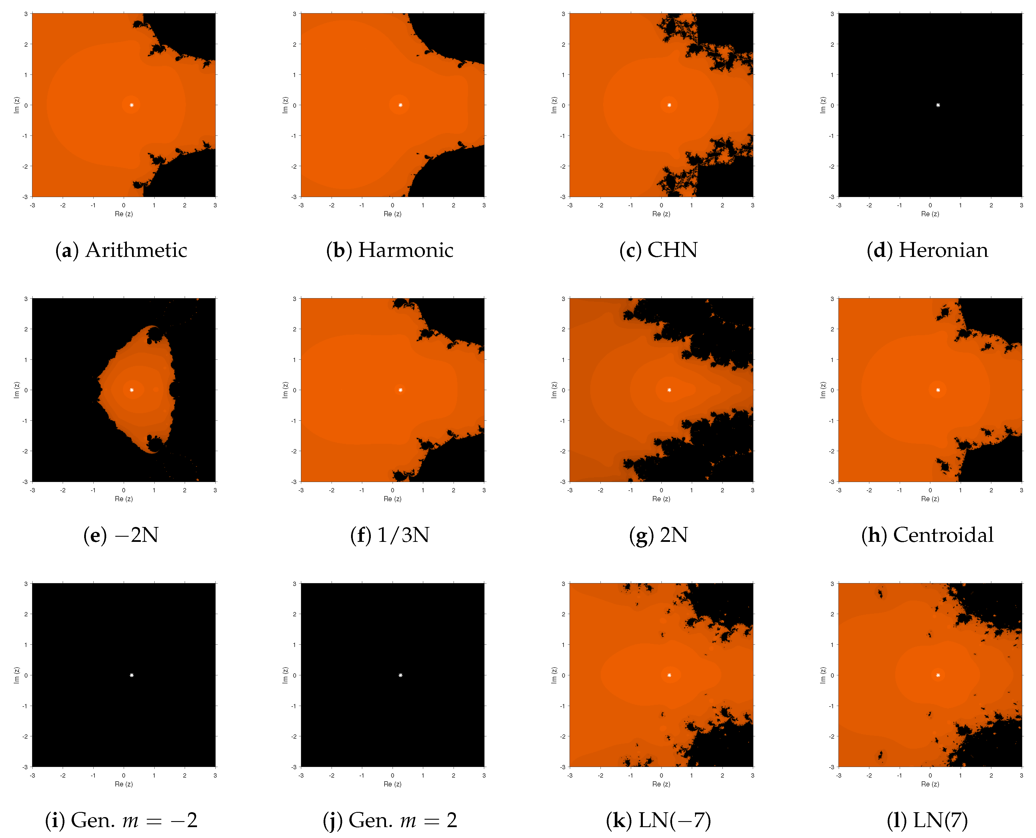
Function $f_3(x)$ had only one zero at $x\approx 0.25753$, whose basin of attraction is painted in orange color in Figure 3. In general, most of the methods presented good performance; however, three methods did not converge to the root in the maximum of iterations required: Heronian and generalized means with $m=\pm 2$. Moreover, the basin of attraction was reduced when the parameter $\theta$ of the convex combination mean was used.

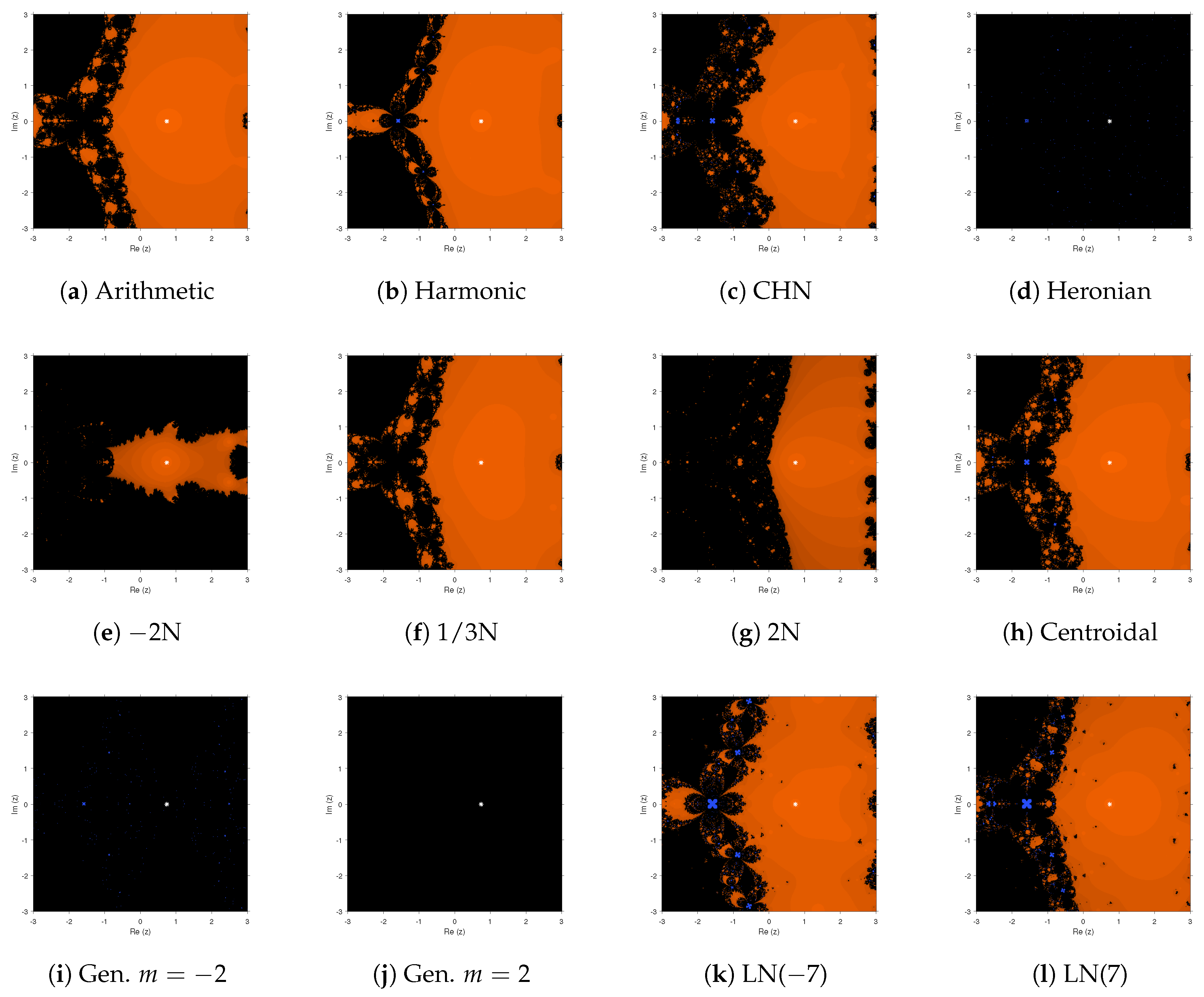
A similar performance is observed in Figure 4, where Heronian and generalized means with $m=\pm 2$ showed no convergence to only the root of $f_4(x)$; meanwhile, the rest of the methods presented good behavior. Let us remark that in some cases, blue areas appear; this corresponded to initial estimations that, after 40 consecutive iterations, had an absolute value higher than 1000. In these cases, they and the surrounding black areas were identified as regions of divergence of the method. The best methods in this case were associated with the arithmetic and harmonic means.

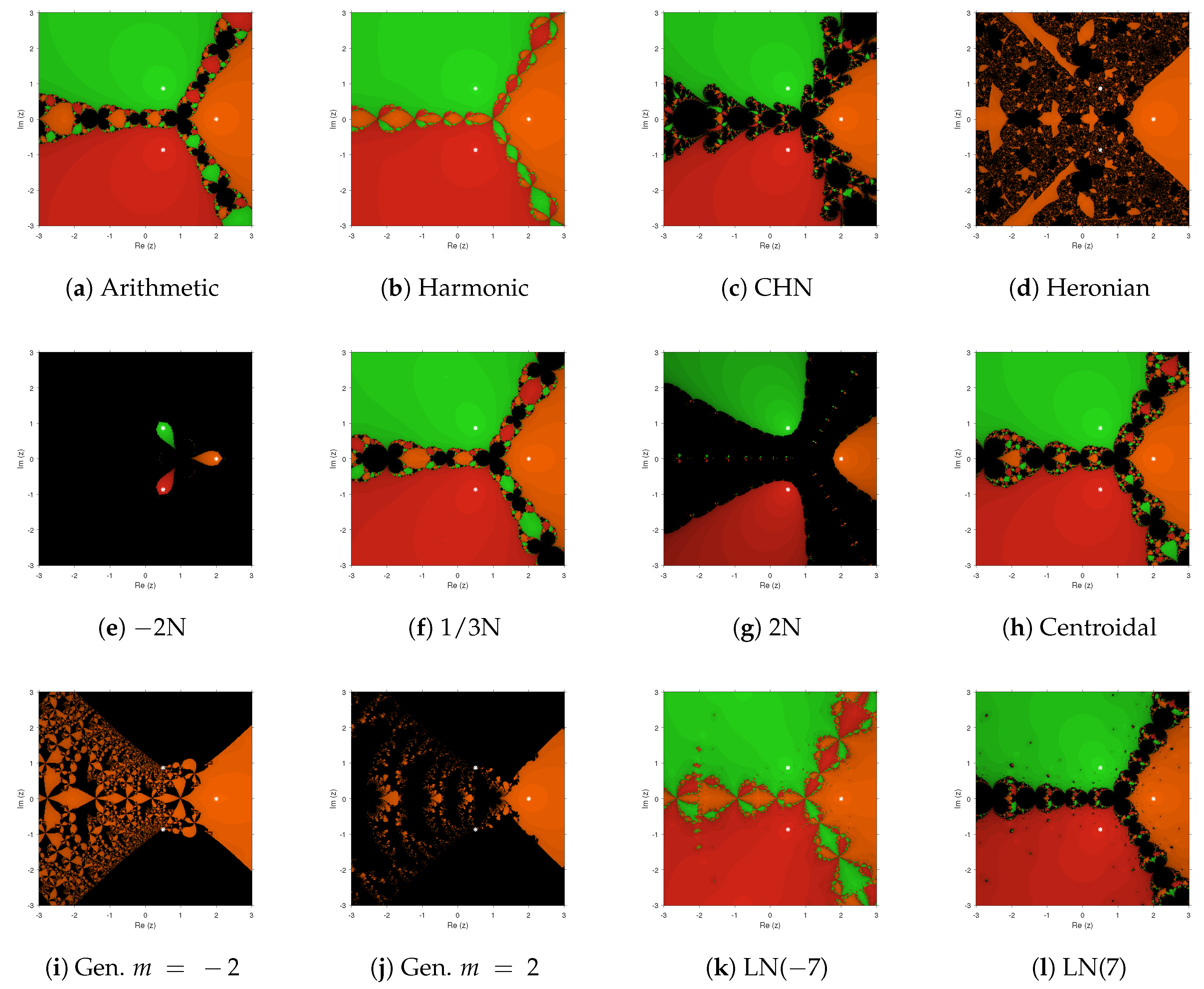
In Figure 5, the best results in terms of the wideness of the basins of the attraction of the roots were for harmonic and Lehmer means, for $m=-7$. The biggest black areas corresponded to convex combination with $\theta =-2$, where the three basins of attraction of the roots were very narrow, and for Heronian and generalized means, there was only convergence to the real root.

5. Conclusions

The proposed $\theta$-test (Corollary 1) has proven to be very useful to reduce the calculations of the analysis of convergence of any MBN. Moreover, though the employment of $\sigma$-means in the context of mean-based variants of Newton’s method is probably not the best one to appreciate their flexibility, their use could still lead to interesting results due to their much greater capability of interpolating between numbers than already powerful means, such as the Lehmer one.

With regard to the numerical performance, Table 1 confirms that a convex combination with a constant coefficient could converge cubically if and only if it was the arithmetic mean; otherwise, as with this case, it converged quadratically, even if it may have done so with less iterations, generally speaking, than CN. Regarding the number of iterations, there were non-linear functions for which LN(m) converged with fewer iterations than HN. In our calculations, we set $m=-7$, but similar results were achieved also for different parameters. Regarding the dependence on initial estimations, the harmonic and Lehmer methods were proven to be very stable, with the widest areas of convergence in most of the nonlinear problems used in the tests.